A PLANAR JITTERING-JETS PATTERN IN CORE COLLAPSE SUPERNOVA EXPLOSIONS
Abstract
We use 3D hydrodynamical numerical simulations and show that jittering bipolar jets that power core-collapse supernova (CCSN) explosions channel further accretion onto the newly born neutron star (NS) such that consecutive bipolar jets tend to be launched in the same plane as the first two bipolar jet episodes. In the jittering-jets model the explosion of CCSNe is powered by jittering jets launched by an intermittent accretion disk formed by accreted gas having a stochastic angular momentum. The first two bipolar jets episodes eject mass mainly from the plane defined by the two bipolar axes. Accretion then proceeds from the two opposite directions normal to that plane. Such a flow has an angular momentum in the direction of the same plane. If the gas forms an accretion disk, the jets will be launched in more or less the same plane as the one defined by the jets of the first two launching episodes. The outflow from the core of the star might have a higher mass flux in the plane define by the jets. In giant stellar progenitors we don’t expect this planar morphology to survive as the massive hydrogen envelope will tend to make the explosion more spherical. In SNe types Ib and Ic, where there is no massive envelope, the planar morphology might have an imprint on the supernova remnant. We speculate that planar jittering-jets are behind the morphology of the Cassiopeia A supernova remnant.
I INTRODUCTION
One class of core collapse supernova (CCSN) explosion models is based on neutrino [7], mainly the delayed neutrino mechanism (e.g., Bethe & Wilson 1, Burrows & Lattimer 4, Burrows et al. 5, Fryer & Warren 14, Ott et al. 35, Marek & Janka 30, Nordhaus et al. 34, Kuroda et al. 24, Hanke et al. 17, Janka 20, Bruenn et al. 3). However, recent 3D numerical studies have shown that the desired explosions are harder to achieve [8, 21, 43] than what 2D numerical simulations had suggested (for a summary of problems of the delayed neutrino mechanism see Papish et al. 40). The problems of the delayed-neutrino mechanism can be overcome if there is a strong wind, either from an accretion disk [23] or from the newly born neutron star (NS). Such a wind is not part of the delayed-neutrino mechanism, and most researchers consider this wind to have a limited contribution to the explosion.
Another class of explosion mechanisms is the jittering-jet scenario [41, 36, 37, 38, 39, 16]. Processes for CCSN explosion by jets were considered before the development of the jittering-jet scenario (e.g. LeBlanc & Wilson 26, Meier et al. 31, Bisnovatyi-Kogan et al. 2, Khokhlov et al. 22, MacFadyen et al. 29, Höflich et al. 19, Woosley & Janka 44, Burrows et al. 6, Couch et al. 10, Couch et al. 9, Lazzati et al. 25). However, most of these MHD models require a rapidly spinning core before collapse starts, and hence are limited to a small fraction of all CCSNe. The jittering-jet scenario posits that all CCSNe are exploded by jets. Recent observations (e.g. Milisavljevic et al. 32, Lopez et al. 28, Ellerbroek et al. 12) show indeed that jets might have a much more general role in CCSNe than what is expected in the neutrino-driven mechanisms and mechanisms that require rapidly rotating cores.
In the jittering-jets scenario the sources of the angular momentum for disk formation are the convective regions in the core [16] and instabilities in the shocked region of the collapsing core, e.g., neutrino-driven convection or the standing accretion shock instability (SASI). Recent 3D numerical simulations show indeed that neutrino-driven convection and SASI are well developed in the first second after core bounce [Hankeetal2013, 43] and the unstable spiral modes of the SASI can amplify magnetic fields [13]. The spiral modes with the amplification of magnetic fields build the ingredients necessary for jets’ launching.
When the average specific angular momentum of the matter in the pre-collapse core is small relative to the amplitude of the specific angular momentum of these instabilities, intermittent jets-launching episodes with random directions occur. The two launching axes of the first two launching episodes define a plane. Using the FLASH numerical code we set a numerical study of the accretion pattern that is likely to be formed after the first two launching episodes. The code and numerical set-up for the 3D simulations are described in section II. The accretion pattern following two jets-launching episodes, followed by a third episode, is described in section III. Our summery is in section IV.
II NUMERICAL SETUP
We study the accretion structure that result from multiple jets-launching episodes using the flash gasdynamical numerical code version 4.2 [15]. The widely used flash code is a publicly available code for supersonic flow suitable for astrophysical applications.
The simulations are done using the split PPM solver of flash. We use 3D Cartesian coordinates with an adaptive mesh refinement (AMR) grid. Fig. 1 shows the resolution in our simulations as a function of distance from the center. In the inner part the cells size is 10 km, increasing with radius.
We treat the spherical inner region of up to from the center as a hole. This means that we are not simulating the NS itself, nor the assumed accretion disk. The boundary condition at the edge of the hole is inflow only, meaning the velocity cannot be positive in the radial direction unless we inject a jet at that specific zone.

To check the sensitivity of our simulations to the resolution used we run a test case with higher resolution (see Fig. 1). A compression with the higher resolution run, that will be presented in section III.5 (Figs. 11, 12), shows that the low and high resolutions runs give results that are within from each other.
We start the simulations after the core has collapsed and bounced back. The initial conditions are taken for a model from the 1D simulations of [27] at a time of after bounce. We map their results into 3D, including the chemical composition. We did not included nuclear reactions in our calcualtions. We set outflow boundary conditions at the exteriors of the simulation’s domain.
In each episode we inject one pair of two opposite jets (bipolar jets). All jets’ axes are in one plane, that we take to be the plane of the numerical Cartesian grid. We take the axis of the numerical grid to be at to the direction of the symmetry axis of the first jets pair. The launching episode results in two opposite jets at some angle from the direction of the first jets. All jets have an initial conical shape, with a half opening angle of .
III ACCRETION PATTERN
III.1 Simulated Cases
We start each simulation by injecting two opposite jets, the first jets’ launching episode. The second bipolar jets pair is injected either at an angle of or relative to the first episode. Each jet launching episode lasts , and the second episode is launched immediately after the end of the first episode. The different simulated cases are summarized in Table 1. The direction of the jets launched in the first two episodes are presented in Fig. 2. Note that in that presentation one of the jets in each pair is represented by two regions.
| Run | |||
|---|---|---|---|
| Active() | |||
| A1 | |||
| A2 | |||
| B1 | |||
| B2 |

III.2 First jet-launching episode
In Fig. 3 we present the density, left panel, and the velocity and temperature, right panel, maps at the end of the first jets launching episode. The flow structure has the typical structure of jet-inflated bubbles (see review by Soker et al. 42). Here we should note the following. () The jets shock material to high temperatures and densities, where nucleosynthesis takes place. These regions have high velocities and can have imprint on the distribution of different isotopes in the SN remnant at later times. This will not be studied here. () The pre-jets flow is that of a collapsing core onto a newly formed NS. After the first jets launching episode accretion continues from directions near the plane perpendicular to the jets’ axis.

Let us elaborate on the accretion pattern. In Fig. 4 we present the inflow mass flux on spheres of radii and . We present the local mass inflow rate , defined as if the entire sphere would have the same inflow mass flux as in the given location,
| (1) |
where and is the density and the radial inward velocity at the point. The first jets pair is able to penetrate thorough the inflowing matter to beyond [39]. As the jets gas is in outflow, it appears as white areas in Fig. 4 and the following similar figures.

III.3 A bipolar accretion pattern
We run two cases of a second jets-launching episode, in directions of (Run A) and (Run B) relative to the direction of the jets’ axis in the first episode. All jets’ axes are in the plane. The density maps, left panels, and the temperature maps with velocity arrows, right panels, of the two cases at the end of the second episode, , are presented in Fig. 5. All plots are in the plane. From these panels, two for each Run, we learn that the strongest inflow is from two opposite directions, through which we draw a dashed line on the density maps of the figure at angles of , and respectively relative to the x-axis.

To identify the inflow pattern of the gas, most of which will be eventually accreted by the NS, we present in Fig. 6 the flow structure in a plane perpendicular to the plane, and cutting it along the dashed lines drawn in the density maps of Fig. 5. Note that the two planes for Run A and Run B are not identical. The left panels of Fig. 6 present the density maps of the two Runs, while the right panels present the inflow mass flux and flow velocity maps. The mass flux is as define in equation (1). In is evident that the inflow close to the NS at the center is mainly from two general opposite directions, the and directions, that are perpendicular to the axes of the two jets’ launching episodes. When the angle between the two first jet-pairs is small, , the high inflow mass flux is from two extended opposite areas. These becomes smaller when the angle between the two episodes are large, . A bipolar accretion flow pattern has emerged.

We can also use the Mollweide-projection (see Fig. 2) to present the emergence of the bipolar inflow (accretion) pattern. This is shown in Fig. 7 for Run A, and in Fig. 8 for Run B. Presented are the inflow mass fluxes on spheres of radii and , as in Fig. 4 for the first jets. Again, the emergence of a bipolar inflow (accretion) structure is evident, particularly in Run B presented in Fig. 8.


III.4 Later evolution
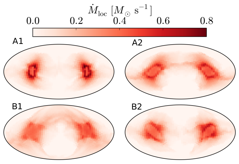
As we discussed in the next section, jets launched by accretion disks formed from the bipolar accretion pattern are likely to be lunched perpendicular to the direction of accretion. Namely, they will be launched in, or close to, the plane defined by the jets’ axes of the first two episodes. We are not in the numerical stage to follow the angular momentum of the accreted gas and from that to find the direction to launch the next jets episode. We therefore arbitrarily run 4 cases for the third jets launching episode as listed in Table 1. In all these cases the third jets launching episode is active in the time period . We present the flow structure for two cases, A1 and B2, in Fig. 9, at the end of the active phase . In all cases we find that a third jets-launching episode strengthens the bipolar accretion pattern and the inflow becomes further concentrated to two opposite directions. In Fig. 10 we use the Mollweide-projection (see Fig. 2) to present the inflow rates through a spheres of radius for the four Runs at the end of the third episode. The jets of the third episode make the bipolar accretion pattern more prominent.

To further quantify the bipolar accretion pattern we construct two opposite cones whose common vertex is at the center, and calculate the ratio of the average inflow mass flux through the cones to the average inflow mass flux through the entire sphere at the same radius. The cones’ axis is perpendicular to the plane, i.e., perpendicular to the jets’ axes, and through the center. The quantity we use is
| (2) |
where is the solid angle covered by the two cones. The evolution of with time for two cone-pairs and at two radii are presented in Fig. 11, for the 4 different Runs listed in Table 1. In one cones pair each cone has an opening angle of , and in the other each cone has an opening angle of . We note that the flow becomes more concentrate, i.e., increases with time, to the perpendicular direction as more jets are launched in the plane. The mass flux per unit solid angle for the cones is substantially larger than that for the cones, . This implies that the inflow has the pattern of two opposite stream columns. This is what we refer to as a bipolar accretion pattern.

.
III.5 Resolution dependency of the results
To check the dependency of our simulations on resolution we ran a test case of case A1 with a higher resolution (see Fig. 1 for the resolution vs radius). We find the accretion rates in the low and high resolution runs to be within of each other, as presented by the thick dashed line in the upper-left panel of Fig. 11. In Fig. 12 we compare the flow structure in the low and high resolution runs at one time. As expected, the features are sharper in the high-resolution run, but the large-scale flow structure is very similar.

We next turn to discuss the implication of the bipolar accretion pattern.
IV IMPLICATIONS AND SUMMARY
In this study we assumed that CCSN explosions are driven by jittering-jets [36], an examined the pattern by which jets are launched. The angular momentum of the core is not large, such that the jets’ axis is determined, at least in part, by stochastic processes such as instabilities and convection in the pre-collapse core [16]. We conducted 3D numerical simulations with the FLASH code [15]. In each jets-launching episode we launched one pair of bipolar jets (Fig. 3). Under these assumptions, the directions of the two first jets-launching episode are more or less random. However, the first two episodes, if not along the same direction, define a plane. We set this plane to be in our study. The jets will eject mass outward along their propagation direction, leaving inflow in perpendicular directions. After the first episode the inflow is from a belt region perpendicular to the jets’ axis, as demonstrated in Fig. 4. After the second episode the inflow is concentrated in two opposite directions, as clearly seen in Figs. 6, 7 and 8. A bipolar accretion flow with its axis perpendicular to the plane has been formed.
An inflowing gas along a direction normal to the plane has an angular momentum direction within that plane. This implies that bipolar accretion flow makes it more likely that the axis of the jets in the third episode will be in the plane, as jets are launched along the angular momentum axis. Namely, the third episode jets’ axis will be in about the same plane as the axes of the first two episodes.
We simulated two directions for the second jets episode, and for each of these we simulated two directions in the same plane for a third jets episode. These four cases are summarized in Table 1. The asymmetry in the accretion flow is presented for these cases in Fig. 11, quantified by the the parameter defined in equation (2). The bipolar pattern becomes more prominent as the inflow becomes more concentrated along two opposite directions. This implies that the following launching of jets will be in, or near, the plane.
The bubbles inflated by the jets grow and expand to all directions as they move toward lower density core gas. Eventually they will close on directions perpendicular to their axis as well, and expel the outer core and the rest of the star in all directions. In addition, some of the jets will not be exactly in the same plane, but will have some stochastic variations from the plane. This will also help in expelling the rest of the star in all directions. This later evolutionary phase will be studied in the future.
Can this planar jittering pattern have any observational consequences? We don’t expect prominent signature in in Type II SNe where the shock will become more spherical as it propagate through the extended massive hydrogen envelope. In type Ic SNe the imprint might exist in the supernova remnant (SNR). We raise here the possibility that the torus morphology of a tilted thick disk with multiple jets in Cassiopeia A SNR (DeLaney et al. 11, Milisavljevic & Fesen 33) is a result of a planar jittering pattern. The last jet was more free to expand, as all core has been removed, and it is now observed as the high velocity jet like outflow along the northeast direction of the SNR.
Finally, we point out that a planar jet launching patter might have taken place during galaxy formation, where a feedback between accretion of cold gas and jet activity might have taken place.
We thank the referee, Jason Nordhaus, for helpful comments. This research was supported by the Asher Fund for Space Research at the Technion, and a generous grant from the president of the Technion Prof. Peretz Lavie. OP is supported by the Gutwirth Fellowship. The software used in this work was developed in part by the DOE NNSA ASC- and DOE Office of Science ASCR-supported Flash Center for Computational Science at the University of Chicago. This work was supported by the Cy-Tera Project (ΝΕΑ /0308/31), which is co-funded by the European Regional Development Fund and the Republic of Cyprus through the Research Promotion Foundation.
References
- [1] Bethe, H. A., & Wilson, J. R. 1985, ApJ, 295, 14
- [2] Bisnovatyi-Kogan, G. S., Popov, I. P., & Samokhin, A. A. 1976, Ap&SS, 41, 287
- [3] Bruenn, S. W., Mezzacappa, A., Hix, W. R., et al. 2013, ApJ, 767, L6
- [4] Burrows, A., & Lattimer, J. M. 1985, ApJ, 299, L19
- [5] Burrows, A., Hayes, J., & Fryxell, B. A. 1995, ApJ, 450, 830
- [6] Burrows, A., Dessart, L., Livne, E., Ott, C. D., & Murphy, J. 2007, ApJ, 664, 416
- [7] Colgate, S. A., & White, R. H. 1966, ApJ, 143, 626
- [8] Couch, S. 2013, Presented in the Fifty-one erg meeting, Raleigh, May 2013.
- [9] Couch, S. M., Pooley, D., Wheeler, J. C., & Milosavljević, M. 2011, ApJ, 727, 104
- [10] Couch, S. M., Wheeler, J. C., & Milosavljević, M. 2009, ApJ, 696, 953
- [11] DeLaney, T., Rudnick, L., Stage, M. D., et al. 2010, ApJ, 725, 2038
- [12] Ellerbroek, L. E., Podio, L., Kaper, L., et al. 2013, A&A, 551, A5
- [13] Endeve, E., Cardall, C. Y., Budiardja, R. D., Beck, S. W., Bejnood, A., Toedte, R. J., Mezzacappa, A., & Blondin, John M.. 2012, ApJ, 751, 26
- [14] Fryer, C. L., & Warren, M. S. 2002, ApJ, 574, L65
- [15] Fryxell, B., Olson, K., Ricker, P., et al. 2000, ApJS, 131, 273
- [16] Gilkis, A., & Soker, N. 2014, MNRAS, 439, 4011
- [17] Hanke, F., Marek, A., Müller, B., & Janka, H.-T. 2012, ApJ, 755, 138
- [18] Hanke, F., Müller, B., Wongwathanarat, A., Marek, A., & Janka, H.-T. 2013, ApJ, 770, 66
- [19] Höflich, P., Khokhlov, A., & Wang, L. 2001, 20th Texas Symposium on relativistic astrophysics, 586, 459
- [20] Janka, H.-T. 2012, Annual Review of Nuclear and Particle Science, 62, 407
- [21] Janka et al. 2013, Presented in the Fifty-one erg meeting, Raleigh, May 2013.
- [22] Khokhlov, A. M., Höflich, P. A., Oran, E. S., et al. 1999, ApJ, 524, L107
- [23] Kohri, K., Narayan, R., & Piran, T. 2005, ApJ, 629, 341
- [24] Kuroda, T., Kotake, K., & Takiwaki, T. 2012, ApJ, 755, 11
- [25] Lazzati, D., Morsony, B. J., Blackwell, C. H., & Begelman, M. C. 2012, ApJ, 750, 68
- [26] LeBlanc, J. M., & Wilson, J. R. 1970, ApJ, 161, 541
- [27] Liebendörfer, M., Rampp, M., Janka, H.-T., & Mezzacappa, A. 2005, ApJ, 620, 840
- [28] Lopez, L. A., Ramirez-Ruiz, E., Castro, D., & Pearson, S. 2013, ApJ, 764, 50
- [29] MacFadyen, A. I., Woosley, S. E., & Heger, A. 2001, ApJ, 550, 410
- [30] Marek, A., & Janka, H.-T. 2009, ApJ, 694, 664
- [31] Meier, D. L., Epstein, R. I., Arnett, W. D., & Schramm, D. N. 1976, ApJ, 204, 869
- [32] Milisavljevic, D., Soderberg, A. M., Margutti, R., et al. 2013, ApJ, 770, L38
- [33] Milisavljevic, D., & Fesen, R. A. 2013, ApJ, 772, 134
- [34] Nordhaus, J., Burrows, A., Almgren, A., & Bell, J. 2010, ApJ, 720, 694
- [35] Ott, C. D., Burrows, A., Dessart, L., & Livne, E. 2008, ApJ, 685, 1069
- [36] Papish, O., & Soker, N. 2011, MNRAS, 1321
- [37] Papish, O., & Soker, N. 2012a, Death of Massive Stars: Supernovae and Gamma-Ray Bursts, 279, 377
- [38] Papish, O., & Soker, N. 2012b, MNRAS, 421, 2763
- [39] Papish, O., & Soker, N. 2014, MNRAS, 438, 1027
- [40] Papish, O., Nordhaus, J., & Soker, N. 2014, arXiv:1402.4362
- [41] Soker, N. 2010, MNRAS, 401, 2793
- [42] Soker, N., Akashi, M., Gilkis, A., et al. 2013, Astronomische Nachrichten, 334, 402
- [43] Takiwaki, T., Kotake, K., & Suwa, Y. 2014, ApJ, 786, 83
- [44] Woosley, S., & Janka, T. 2005, Nature Physics, 1, 147