A Discrete Method to Solve Fractional
Optimal Control ProblemsThanks: This is
a preprint of a paper whose final and definite form will appear in
Nonlinear Dynamics, ISSN 0924-090X. Paper submitted 26/Nov/2013;
revised 17/March/2014; accepted for publication 20/March/2014.
Department of Mathematics, University of Aveiro, 3810–193 Aveiro, Portugal
Abstract
We present a method to solve fractional optimal control problems, where the dynamic depends on integer and Caputo fractional derivatives. Our approach consists to approximate the initial fractional order problem with a new one that involves integer derivatives only. The latter problem is then discretized, by application of finite differences, and solved numerically. We illustrate the effectiveness of the procedure with an example.
Mathematics Subject Classification 2010: 26A33, 49M25.
Keywords: fractional calculus, fractional optimal control, direct methods.
1 Introduction
The fractional calculus deals with differentiation and integration of arbitrary (noninteger) order [15]. It has received an increasing interest due to the fact that fractional operators are defined by natural phenomena [3].
A particularly interesting, and very active, research area is that of the fractional optimal control, where the dynamic control system involves not only integer order derivatives but fractional operators as well [9, 14]. Such fractional problems are difficult to solve and numerical methods are often applied, which have proven to be efficient and reliable [1, 4, 5, 8, 13]. Typically, using an approximation for the fractional operators, the fractional optimal control problem is rewritten into a new one, that depends on integer derivatives only [2, 12]. Then, using necessary optimality conditions, the problem is reduced to a system of ordinary differential equations and, by finding its solution, one approximates the solution to the original fractional problem [12]. Our approach is different here: after replacing the fractional operator, we consider the augmented functional and apply an Euler-like method.
2 Preliminaries
We start with some definitions needed in the sequel. For more on the subject we refer the reader to [7, 9, 10, 15].
Definition 1.
Let and be the order of the integral or the derivative. For , we define
- 1.
the left Riemann–Liouville fractional integral by
- 2.
the right Riemann–Liouville fractional integral by
- 3.
the left Riemann–Liouville fractional derivative by
- 4.
the right Riemann–Liouville fractional derivative by
- 5.
the left Caputo fractional derivative by
- 6.
the right Caputo fractional derivative by
where for the definitions of Riemann–Liouville fractional derivatives, and
| (1) |
for the Caputo fractional derivatives.
When is an integer, the operators of Definition 1 reduce to standard ones:
There is an useful relation between Riemann–Liouville and Caputo fractional derivatives:
| (2) |
For numerical purposes, approximations are used to deal with these fractional operators. The Riemann–Liouville derivatives are expandable in a power series involving integer order derivatives only. If is an analytic function, then (cf. [7])
| (3) |
where
The obvious disadvantage of using (3) in numerical computations is that in order to have a small error, one has to sum a large number of terms and thus the function has to possess higher-order derivatives, which is not suitable for optimal control. To address this problem, a second approach was carried out in [2, 12], where a good approximation is obtained without the requirement of such higher-order smoothness on the admissible functions. The method can be explained, for left-derivatives, in the following way. Let and . Then,
where is the solution of the system
for and , and are given by
Using (2), a similar formula can be deduced for the Caputo fractional derivative. When we consider finite sums only, that is, when we use the approximation
| (4) |
where and
the error is bounded by
See [12] for proofs and other details.
3 Problem Statement and the Approximation Method
The fractional optimal control problem that we consider here is the following one. Let be the fixed fractional order, and consider two differentiable functions and with domain . Minimize the functional
subject to the fractional dynamic constraint
and the initial condition
where and is a fixed real number. Two situations are considered: fixed or free. Sufficient and necessary conditions to obtain solutions for this problem were studied in [14]. Here we proceed with a different approach. First, we replace the operator with the approximation given in (4). With relation (2) we get
where, for simplicity,
Thus, one has
Define the vector
and the new function
We construct a new optimal control problem: minimize the functional
| (5) |
subject to the dynamic constraints
| (6) |
and the initial conditions
| (7) |
To solve the problem (5)–(7), one can consider the Hamiltonian function
where denotes the Lagrange multipliers,
By the Pontryagin maximum principle [11], to solve the problem one should solve the following system of ODEs:
subject to the boundary conditions
if is free, or
otherwise. Instead of this indirect approach, we apply here a direct method, based on an Euler discretization, to obtain a finite-dimensional approximation of the continuous problem (5)–(7). We summarize briefly the method. Consider a finite grid
where, for simplicity, is assumed constant for all . Each dynamic constraint is approximated by
and
where
The integral
in replaced by the Riemann sum
The finite version of problem (5)–(7) is the following one: minimize
subject to the dynamic constraints
and the initial conditions
( fixed or free). In the next section we illustrate the method with an example.
4 An Illustrative Example
In this section we exemplify the procedure of Section 3 with a concrete example. To start, we recall the Caputo fractional derivative of a power function (cf. Property 2.16 of [7]). Let be arbitrary, with given by (1), and define . Then,
Assume that we wish to minimize the functional
| (8) |
subject to the dynamic constraint
| (9) |
and the boundary conditions
| (10) |
The solution is the pair
| (11) |
Indeed, (11) satisfies both constraints (9) and (10) with while functional (8) is non-negative: for all admissible pairs . After replacing the fractional derivative by the appropriate approximation, and fixing , we get the following problem: minimize the functional
| (12) |
subject to the dynamic constraints
| (13) |
and the boundary conditions
| (14) |
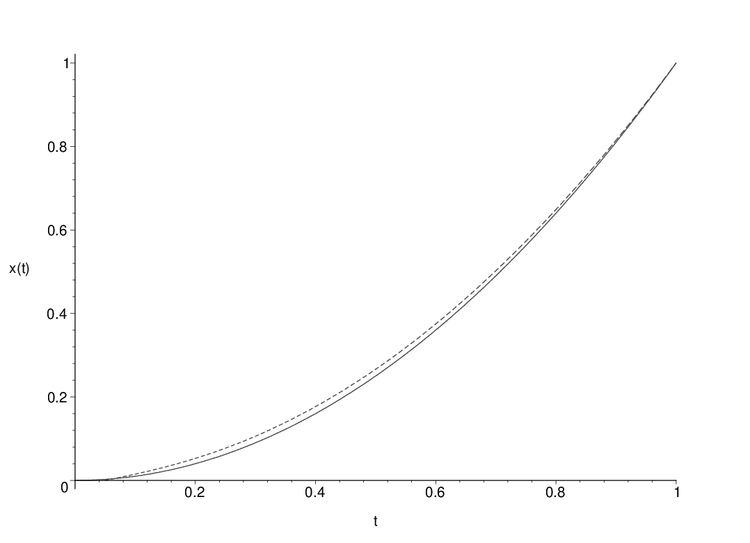
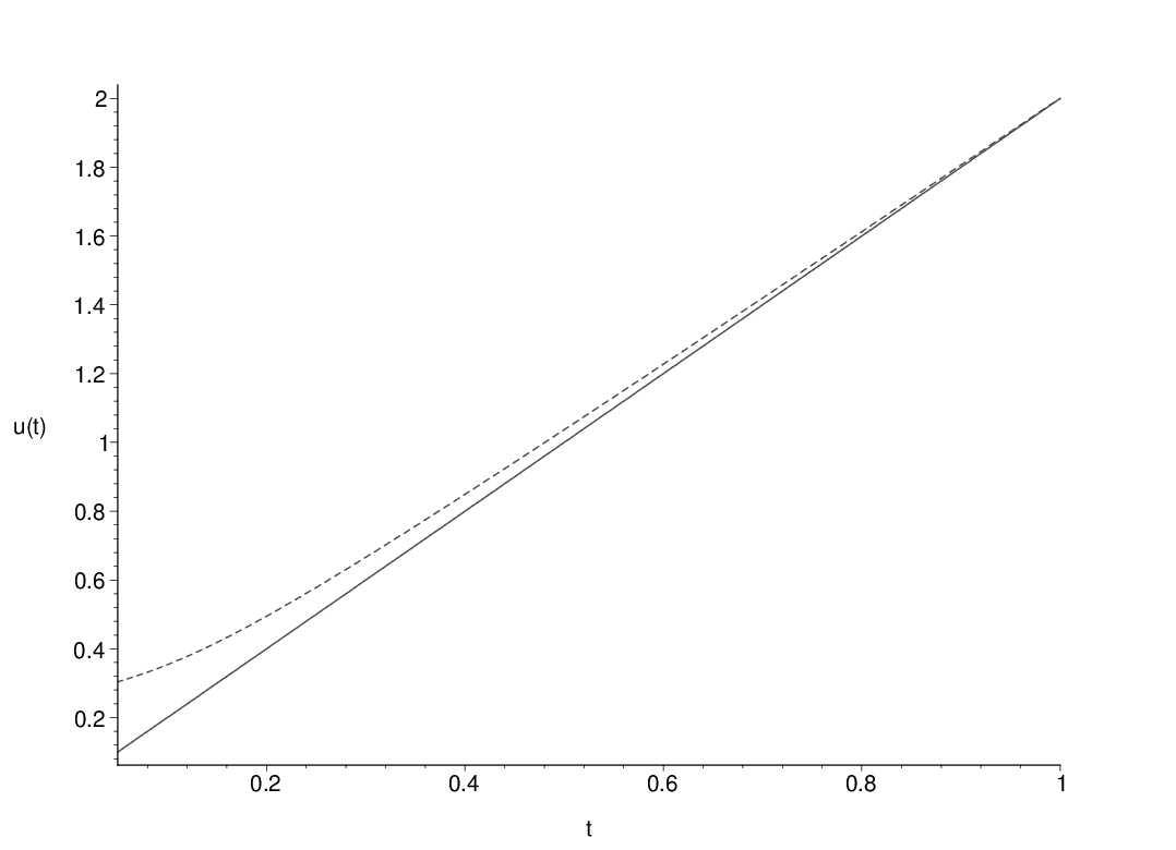
We apply a direct method to the previous problem, also called a “first discretize then optimize method”. More precisely, the objective functional (12) and the system of ODEs (14) were discretized by a simple Euler method with fixed step size, as explained in Section 3. Then we solved the resulting nonlinear programming problem by using the AMPL modeling language for mathematical programming [6] in connection with IPOPT of Wächter and Biegler [16]. In Figure 1a we show the results for the state function and in Figure 1b we show the results for the control function , where we have used and .
Acknowledgments
This article was supported by Portuguese funds through the Center for Research and Development in Mathematics and Applications (CIDMA), and The Portuguese Foundation for Science and Technology (FCT), within project PEst-OE/MAT/UI4106/2014. Torres was also supported by the FCT project PTDC/EEI-AUT/1450/2012, co-financed by FEDER under POFC-QREN with COMPETE reference FCOMP-01-0124-FEDER-028894.
References
- [1] M. Aoun, R. Malti, F. Levron and A. Oustaloup, Numerical simulations of fractional systems: An overview of existing methods and improvements, Nonlinear Dynam. 38 no. 1-4 (2004), 117–131.
- [2] T. M. Atanackovic and B. Stankovic, On a numerical scheme for solving differential equations of fractional order, Mech. Res. Comm. 35 (2008), no. 7, 429–438.
- [3] D. A. Benson, M. M. Meerschaert and J. Revielle, Fractional calculus in hydrologic modeling: A numerical perspective, Advances in Water Resources 51 (2013), 479–497.
- [4] N. J. Ford and M. L. Morgado, Fractional boundary value problems: analysis and numerical methods, Fract. Calc. Appl. Anal. 14 (2011), no. 4, 554–567.
- [5] N. J. Ford and M. L. Morgado, Distributed order equations as boundary value problems, Comput. Math. Appl. 64 (2012), no. 10, 2973–2981.
- [6] R. Fourer, D. M. Gay and B. W. Kernighan, AMPL: A modeling language for mathematical programming, Duxbury Press, Brooks/Cole Publishing Company, 2002.
- [7] A. A. Kilbas, H. M. Srivastava and J. J. Trujillo, Theory and applications of fractional differential equations, North-Holland Mathematics Studies, 204, Elsevier, Amsterdam, 2006.
- [8] A. Lotfi, M. Dehghan and S. A. Yousefi, A numerical technique for solving fractional optimal control problems, Comput. Math. Appl. 62 (2011), no. 3, 1055–1067.
- [9] A. B. Malinowska and D. F. M. Torres, Introduction to the fractional calculus of variations, Imp. Coll. Press, London, 2012.
- [10] I. Podlubny, Fractional differential equations, Mathematics in Science and Engineering, 198, Academic Press, San Diego, CA, 1999.
- [11] L. S. Pontryagin, V. G. Boltyanskii, R. V. Gamkrelidze and E. F. Mishchenko, The mathematical theory of optimal processes, Translated from the Russian by K. N. Trirogoff; edited by L. W. Neustadt Interscience Publishers John Wiley & Sons, Inc. New York, 1962.
- [12] S. Pooseh, R. Almeida and D. F. M. Torres, Numerical approximations of fractional derivatives with applications, Asian J. Control 15 (2013), no. 3, 698–712. arXiv:1208.2588
- [13] S. Pooseh, R. Almeida and D. F. M. Torres, Discrete direct methods in the fractional calculus of variations, Comput. Math. Appl. 66 (2013), no. 5, 668–676. arXiv:1205.4843
- [14] S. Pooseh, R. Almeida and D. F. M. Torres, Fractional order optimal control problems with free terminal time, J. Ind. Manag. Optim. 10 (2014), no. 2, 363–381. arXiv:1302.1717
- [15] S. G. Samko, A. A. Kilbas and O. I. Marichev, Fractional integrals and derivatives, translated from the 1987 Russian original, Gordon and Breach, Yverdon, 1993.
- [16] A. Wächter and L. T. Biegler, On the implementation of an interior-point filter line-search algorithm for large-scale nonlinear programming, Math. Program. 106 (2006), no. 1, Ser. A, 25–57.