跳到论文正文
W Papers独立论文阅读器 arXiv:1403.4982 论文正文 计算阅读时间 · 0%
引用这篇论文根据当前论文元数据生成,正式投稿前建议核对。


License: arXiv.org perpetual non-exclusive license
arXiv:1403.4982v1 [math.SG] 19 Mar 2014

Augmentations and Rulings of Legendrian Knots

C. Leverson Address: Duke University, Durham, NC 27708 Email address: cleverso@math.duke.edu
Date: August 24, 2026
Abstract.

For any Legendrian knot Λ\Lambda in (ℝ3,ker​(d​z−y​d​x))({\mathbb{R}}^{3},{\hbox{ker}}\,(dz-ydx)), we show that the existence of an augmentation to any field of the Chekanov-Eliashberg differential graded algebra over ℤ⁡[t,t−1]{\mathbb{Z}}[t,t^{-1}] is equivalent to the existence of a ruling of the front diagram, generalizing results of Fuchs, Ishkhanov, and Sabloff. We also show that any even graded augmentation must send tt to −1-1.

1. Introduction

A Legendrian knot in (ℝ3,ξstd)({\mathbb{R}}^{3},\xi_{\text{std}}) is an embedding Λ:S1→ℝ3\Lambda:S^{1}\to{\mathbb{R}}^{3} which is everywhere tangent to the contact planes. In [4] (see related [6]), Chekanov introduced a combinatorial way to associate a non-commutative differential graded algebra (DGA) over ℤ/2{\mathbb{Z}}/2 to a Lagrangian diagram of a Legendrian knot Λ\Lambda in ℝ3{\mathbb{R}}^{3}. The DGA is generated by crossings of Λ\Lambda and the differential is determined by a count of immersed polygons whose edges lie on the knot and whose corners lie at crossings of Λ\Lambda. In the literature, this DGA is called the Chekanov-Eliashberg DGA. Chekanov showed that the homology of the DGA is invariant under Legendrian isotopy. He also showed that a linearized version of the homology of the DGA could be used to distinguish between two Legendrian 525_{2} knots in ℝ3{\mathbb{R}}^{3} which could not be distinguished by the rotation and Thurston-Bennequin numbers. In the early 2000’s, Etnyre, Ng, and Sabloff gave a lift of the Chekanov-Eliashberg DGA to a DGA (𝒜R,∂)(\mathcal{A}_{R},\partial) over R=ℤ⁡[t,t−1]R={\mathbb{Z}}[t,t^{-1}] which has a full ℤ{\mathbb{Z}}-grading (see [10]). One can recover the Chekanov-Eliashberg DGA by setting t=1t=1, which requires one to consider the grading mod 2​r​(Λ)2r(\Lambda), and considering the coefficients mod 22 (where r⁡(Λ)r(\Lambda) is the rotation number, defined in §2).

Another Legendrian knot invariant uses generating families, functions whose critical values generate front diagrams of Legendrian knots. Following ideas introduced by Eliashberg in [5], Fuchs [11] and Chekanov-Pushkar [3] gave invariants involving decompositions of the generating families, which are now called “normal rulings” and can also be used to distinguish between Chekanov’s 525_{2} knots.

Remarkably, there is a close connection between the Chekanov-Eliashberg DGA and rulings. Fuchs [11], Fuchs-Ishkhanov [12], and Sabloff [17] showed that the existence of a ruling is equivalent to the existence of an augmentation to ℤ/2{\mathbb{Z}}/2 of the Chekanov-Eliashberg DGA, where an augmentation to a ring SS is an algebra map ϵ:𝒜R→S\epsilon:\mathcal{A}_{R}\to S such that ϵ∘∂=0\epsilon\circ\partial=0 and ϵ⁡(1)=1\epsilon(1)=1.

The main result of this paper gives a generalization of these results using an extension of Sabloff’s construction in [17]. Let FF be a field and R=ℤ⁡[t,t−1]R={\mathbb{Z}}[t,t^{-1}]. Given a ρ\rho-graded augmentation ϵ:𝒜R→F\epsilon:\mathcal{A}_{R}\to F of the ℤ⁡[t,t−1]{\mathbb{Z}}[t,t^{-1}]-differential graded algebra (𝒜R,∂)(\mathcal{A}_{R},\partial) of a knot Λ\Lambda, we will find a ρ\rho-graded normal ruling of the knot diagram. Conversely, given a ρ\rho-graded normal ruling of the knot diagram, we will define a ρ\rho-graded augmentation ϵ:𝒜R→F\epsilon:\mathcal{A}_{R}\to F of the DGA over ℤ⁡[t,t−1]{\mathbb{Z}}[t,t^{-1}] with ϵ⁡(t)=−1\epsilon(t)=-1. (For ρ=0\rho=0, this is the so called graded case and for ρ=1\rho=1, the ungraded case.) Terminology will be introduced in §2.

In §3 and §4, we will show:

Theorem 1.1.

Let Λ\Lambda be a Legendrian knot in ℝ3{\mathbb{R}}^{3}. Given a field FF, (𝒜R,∂)(\mathcal{A}_{R},\partial) has a ρ\rho-graded augmentation ϵ:𝒜R→F\epsilon:\mathcal{A}_{R}\to F if and only if any front diagram of Λ\Lambda has a ρ\rho-graded normal ruling. Furthermore, if ρ\rho is even, then ϵ⁡(t)=−1\epsilon(t)=-1.

Note that this generalizes Fuchs, Fuchs-Ishkhanov, and Sabloff’s results, giving a correspondence between normal rulings and augmentations to any field FF of the DGA over ℤ⁡[t,t−1]{\mathbb{Z}}[t,t^{-1}]. This does not contradict the result in [15] that there are augmentations to matrix algebras which do not send tt to −1-1 as the matrix algebras are not fields.

Theorem 1.1 can be extended and interpreted in terms of the augmentation variety for a Legendrian knot. Define

Augρ(Λ)={ϵ(t):ϵ a ρ-graded augmentation of (𝒜R,∂)}⊂F∗\operatorname{Aug}_{\rho}(\Lambda)=\{\epsilon(t):\epsilon\text{ a $\rho$-graded augmentation of }(\mathcal{A}_{R},\partial)\}\subset F^{*}

the augmentation variety of Λ\Lambda, where F∗=F\{0}F^{*}=F\backslash\{0\}.

In higher dimensions, understanding the augmentation variety is interesting and useful (see [1] and [14]), so there has been some question as to whether we can determine the augmentation variety in ℝ3{\mathbb{R}}^{3} with the standard contact structure. In §3, we prove:

Theorem 1.2.

If ρ\rho is odd and ρ|2​r​(Λ)\rho|2r(\Lambda), then

Augρ(Λ)={{−x2:x∈F∗}OPEN if there exists a ​ρ​-graded normal ruling of Λ which is not oriented (introduced in §3){−1} if there exists a ​ρ​-graded normal ruling of ​Λ​ and all rulings are oriented∅ if there are no ρ-graded normal rulings of Λ.\operatorname{Aug}_{\rho}(\Lambda)=\begin{cases}\{-x^{2}:x\in F^{*}\}&\text{ if there exists a }\rho\text{-graded normal ruling of $\Lambda$ which is not oriented (introduced in \lx@sectionsign\ref{sec:augRuling}})\\ \{-1\}&\text{ if there exists a }\rho\text{-graded normal ruling of }\Lambda\text{ and all rulings are oriented}\\ \emptyset&\text{ if there are no }\rho\text{-graded normal rulings of }\Lambda.\end{cases}

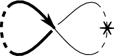
For example, the right handed trefoil Λ\Lambda in Figure 1 has DGA (𝒜R,∂)(\mathcal{A}_{R},\partial) with |ci|=0\lvert c_{i}\rvert=0 for 1≤i≤31\leq i\leq 3, |c4|=|c5|=1\lvert c_{4}\rvert=\lvert c_{5}\rvert=1, and |t|=0\lvert t\rvert=0. Then 𝒜R=𝒜R​(c1,…,c5)\mathcal{A}_{R}=\mathcal{A}_{R}(c_{1},\ldots,c_{5}) with differential

∂c1\displaystyle\partial c_{1} =∂c2=∂c3=0\displaystyle=\partial c_{2}=\partial c_{3}=0
∂c4\displaystyle\partial c_{4} =t+c1+c3+c1​c2​c3\displaystyle=t+c_{1}+c_{3}+c_{1}c_{2}c_{3}
∂c5\displaystyle\partial c_{5} =1−c1−c3−c3​c2​c1.\displaystyle=1-c_{1}-c_{3}-c_{3}c_{2}c_{1}.

Let FF be a field. If ϵ:𝒜R→F\epsilon:\mathcal{A}_{R}\to F is a 11-graded (ungraded) augmentation, then

0\displaystyle 0 =ϵ⁡(t)+ϵ⁡(c1)+ϵ⁡(c3)+ϵ⁡(c1)​ϵ​(c2)​ϵ​(c3)\displaystyle=\epsilon(t)+\epsilon(c_{1})+\epsilon(c_{3})+\epsilon(c_{1})\epsilon(c_{2})\epsilon(c_{3})
0\displaystyle 0 =1−ϵ⁡(c1)−ϵ⁡(c3)−ϵ⁡(c3)​ϵ​(c2)​ϵ​(c1)\displaystyle=1-\epsilon(c_{1})-\epsilon(c_{3})-\epsilon(c_{3})\epsilon(c_{2})\epsilon(c_{1})

and so ϵ⁡(t)=−1\epsilon(t)=-1. Thus Aug1⁡(Λ)={−1}\operatorname{Aug}_{1}(\Lambda)=\{-1\}.

Now consider the left handed trefoil Λ′\Lambda^{\prime} depicted in Figure 1. The associated DGA is (𝒜R′,∂′)(\mathcal{A}_{R}^{\prime},\partial^{\prime}) with |c1|=|c2|=|c4|=−1\lvert c_{1}\rvert=\lvert c_{2}\rvert=\lvert c_{4}\rvert=-1, |c3|=|c5|=|c6|=1\lvert c_{3}\rvert=\lvert c_{5}\rvert=\lvert c_{6}\rvert=1, and |t|=2\lvert t\rvert=2. Then 𝒜R=𝒜R​(c1,…,c6)\mathcal{A}_{R}=\mathcal{A}_{R}(c_{1},\ldots,c_{6}) with differential

∂′c1\displaystyle\partial^{\prime}c_{1} =∂′c2=∂′c3=0\displaystyle=\partial^{\prime}c_{2}=\partial^{\prime}c_{3}=0
∂′c4\displaystyle\partial^{\prime}c_{4} =t+c1​c2\displaystyle=t+c_{1}c_{2}
∂′c5\displaystyle\partial^{\prime}c_{5} =1+c2​c3\displaystyle=1+c_{2}c_{3}
∂′c6\displaystyle\partial^{\prime}c_{6} =1+c3​c1.\displaystyle=1+c_{3}c_{1}.

Let FF be a field. If ϵ:𝒜R′→F\epsilon:\mathcal{A}_{R}^{\prime}\to F is a 11-graded (ungraded) augmentation, then

0\displaystyle 0 =ϵ⁡(t)+ϵ⁡(c1)​ϵ​(c2)\displaystyle=\epsilon(t)+\epsilon(c_{1})\epsilon(c_{2})
0\displaystyle 0 =1+ϵ⁡(c2)​ϵ​(c3)\displaystyle=1+\epsilon(c_{2})\epsilon(c_{3})
0\displaystyle 0 =1+ϵ⁡(c3)​ϵ​(c1).\displaystyle=1+\epsilon(c_{3})\epsilon(c_{1}).

Therefore ϵ⁡(c2)=−(ϵ⁡(c3))−1=ϵ⁡(c1)\epsilon(c_{2})=-(\epsilon(c_{3}))^{-1}=\epsilon(c_{1}) and so ϵ⁡(t)=−(ϵ⁡(c3))−2\epsilon(t)=-(\epsilon(c_{3}))^{-2}. So any nonzero choice of ϵ⁡(c3)\epsilon(c_{3}) yields an augmentation and thus Aug1⁡(Λ′)={−x2:x∈F∗}\operatorname{Aug}_{1}(\Lambda^{\prime})=\{-x^{2}:x\in F^{*}\}.

\labellist\pinlabel

c1c_{1} [b] at 44 288 \pinlabelc2c_{2} [b] at 256 290 \pinlabelc3c_{3} [b] at 447 289 \pinlabelc4c_{4} [b] at 543 389 \pinlabelc5c_{5} [t] at 546 160

\pinlabel

c1c_{1} [br] at 1145 240 \pinlabelc2c_{2} [bl] at 1318 240 \pinlabelc3c_{3} [t] at 1225 96 \pinlabelc4c_{4} [r] at 1220 392 \pinlabelc5c_{5} [tr] at 1398 91 \pinlabelc6c_{6} [tl] at 1060 95 \endlabellist

Refer to caption
Figure 1. The left figure is a Legendrian right handed trefoil and the right is a Legendrian left handed trefoil with crossings labeled. The ∗* indicates the placement of the base point corresponding to tt.

This result complements the recent work of Henry and Rutherford [13]. Henry and Rutherford show that counts of the augmentations to any finite field, without restrictions on where the augmentation sends tt, are Legendrian knot invariants and that they can be related to the ruling polynomials of the knot, thus showing that the Chekanov-Eliashberg algebra determines the ruling polynomial. Our result shows that if ρ\rho is even, one can restrict the count of ρ\rho-graded augmentations to augmentations which send tt to −1-1, as there are not any which do not.

Theorem 1.1 tells us that if there exists an augmentation to ℤ/2{\mathbb{Z}}/2, then there exists an augmentation to any field. In §5, we will show that given an augmentation to ℤ/2{\mathbb{Z}}/2 of the Chekanov-Eliashberg DGA, we can use constructions similar to those in the proof of Theorem 1.1 to define an augmentation to any ring. In particular:

Theorem 1.3.

Let Λ\Lambda be a Legendrian knot in ℝ3{\mathbb{R}}^{3}. Let (𝒜ℤ/2,∂)(\mathcal{A}_{{\mathbb{Z}}/2},\partial) be the Chekanov-Eliashberg DGA over ℤ/2{\mathbb{Z}}/2 and let (𝒜R,∂)(\mathcal{A}_{R},\partial) be the DGA over R=ℤ⁡[t,t−1]R={\mathbb{Z}}[t,t^{-1}]. If ϵ′:𝒜ℤ/2→ℤ/2\epsilon^{\prime}:\mathcal{A}_{{\mathbb{Z}}/2}\to{\mathbb{Z}}/2 is an augmentation of (𝒜ℤ/2,∂)(\mathcal{A}_{{\mathbb{Z}}/2},\partial), then one can find a lift of ϵ′\epsilon^{\prime} to an augmentation ϵ:𝒜R→ℤ\epsilon:\mathcal{A}_{R}\to{\mathbb{Z}} of (𝒜R,∂)(\mathcal{A}_{R},\partial) such that ϵ⁡(t)=−1\epsilon(t)=-1.

In other words, we will define ϵ\epsilon so that the following diagram commutes:

(𝒜R,∂)\textstyle{(\mathcal{A}_{R},\partial)\ignorespaces\ignorespaces\ignorespaces\ignorespaces\ignorespaces\ignorespaces\ignorespaces\ignorespaces}ϵ\scriptstyle{\epsilon}t=1\scriptstyle{t=1}ℤ\textstyle{{\mathbb{Z}}\ignorespaces\ignorespaces\ignorespaces\ignorespaces}(𝒜ℤ/2,∂)\textstyle{(\mathcal{A}_{{\mathbb{Z}}/2},\partial)\ignorespaces\ignorespaces\ignorespaces\ignorespaces}ϵ′\scriptstyle{\epsilon^{\prime}}ℤ/2\textstyle{{\mathbb{Z}}/2}

This theorem tells us that given an augmentation to ℤ/2{\mathbb{Z}}/2 of (𝒜ℤ/2,∂)(\mathcal{A}_{{\mathbb{Z}}/2},\partial), there exists an augmentation to any ring SS of (𝒜R,∂)(\mathcal{A}_{R},\partial) which sends tt to −1-1.

1.1. Outline of the article

In §2 we recall background on Legendrian knots and give definitions of the Chekanov-Eliashberg DGA, including sign conventions for defining the algebra over ℤ⁡[t,t−1]{\mathbb{Z}}[t,t^{-1}], and a normal ruling. §3 gives the proof that given an augmentation one can define a normal ruling. §4 finishes the proof of Theorem 1.1 by proving that given a normal ruling one can define an augmentation. §4 goes to prove Theorem 1.2, giving the augmentation variety in the odd graded case. The paper concludes with the proof of Theorem 1.3 in §5.

1.2. Acknowledgements

The author thanks Lenhard Ng for introduction to the problem, for many useful discussions, and for the contribution of the proof of Lemma 3.2. The author also thanks Dan Rutherford for helpful conversations. This work was partially supported by NSF grant DMS-0846346.

2. Background Material

2.1. Diagrams of Knots

In this section, we will briefly review necessary ideas of Legendrian knot theory. For further references on this subject, see [8].

A contact structure on a 3-manifold MM is a completely nonintegrable 2-plane field ξ\xi. Locally, a contact structure is the kernel of a 1-form α\alpha which satisfies the non-degeneracy condition

α∧d​α≠0\alpha\wedge d\alpha\neq 0

at every point in MM. We will be concerned with the standard contact structure on ℝ3{\mathbb{R}}^{3}, which is the completely nonintegrable 2-plane field ξ0=ker​α0\xi_{0}={\hbox{ker}}\,\alpha_{0}, where α0=d​z−y​d​x\alpha_{0}=dz-ydx. A Legendrian knot is an embedding Λ:S1→ℝ3\Lambda:S^{1}\to{\mathbb{R}}^{3} which is everywhere tangent to the contact planes. A Legendrian isotopy is an ambient isotopy of Λ\Lambda through Legendrian knots. We are interested in Legendrian isotopy classes of Legendrian knots in ℝ3{\mathbb{R}}^{3}.

The classical invariants for Legendrian isotopy classes of knots are the topological knot type, Thurston-Bennequin number, and rotation number (see [2]). The Thurston-Bennequin number measures the self-linking of a Legendrian knot Λ\Lambda. If Λ′\Lambda^{\prime} is a knot that is a push off of Λ\Lambda in a direction tangent to the contact structure, then t​b​(Λ)tb(\Lambda) is the linking number of Λ\Lambda and Λ′\Lambda^{\prime}. The rotation number rr of an oriented Legendrian knot Λ\Lambda is the rotation of its tangent vector field with respect to any global trivialization of ξ0\xi_{0}, for example, {∂y,∂x+y∂z}\{\partial_{y},\partial_{x}+y\partial_{z}\}. A natural question is then whether these invariants with the topological knot type alone classify Legendrian knots, in other words, whether all Legendrian knots are “Legendrian simple.” Eliashberg and Fraser [7] show that Legendrian unknots are Legendrian simple and Etnyre and Honda [9] show that Legendrian torus and figure eight knots are as well.

Two particularly useful projections of Legendrian knots are the Lagrangian projection and the front projection. The Lagrangian projection is the map

πℓ:(x,y,z)↦(x,y).\pi_{\ell}:(x,y,z)\mapsto(x,y).

The front projection is the map

πf:(x,y,z)↦(x,z).\pi_{f}:(x,y,z)\mapsto(x,z).

In general, we will call the Lagrangian projection (resp. front projection) of a Legendrian knot a Lagrangian diagram (resp. front diagram). Figure 2 gives Lagrangian (left) and front (right) projections of a Legendrian version of a right handed trefoil.

\labellist\hair

2pt \pinlabelc1c_{1} [t] at 50 195 \pinlabelc2c_{2} [t] at 255 195 \pinlabelc3c_{3} [t] at 447 195 \pinlabelq1q_{1} [b] at 545 326 \pinlabelq2q_{2} [t] at 545 92 \endlabellistRefer to caption

Figure 2. The left figure gives a Lagrangian projection of a Legendrian right handed trefoil with crossings labeled and the right figure gives a front projection.

Note that one can recover the yy coordinate of a knot from the slope of the front diagram (see [8]):

y=d​zd​x.y=\frac{dz}{dx}.

This implies that lines tangent to a front diagram of a Legendrian knot are never vertical. Front diagrams instead have semicubical cusps. It also implies that at a double point the strand with the smaller (more negative) slope has a smaller yy coordinate and so passes in front of the strand with larger (more positive) slope. For a front diagram of an oriented Legendrian knot, the rotation number is half of the difference between the number of downward-pointing cusps and the number of upward-pointing cusps.

In particular, we will find that front diagrams in plat position will be easier to manipulate. A front diagram is in plat position if all of the left cusps have the same xx coordinate, all of the right cusps have the same xx coordinate, and there do not exist crossings in the diagram which have the same xx coordinate. One can use Legendrian versions of the Reidemeister II moves and planar isotopy to put any front diagram into plat position. The diagram of the trefoil given in Figure 2 is an example of a diagram in plat position.

2.2. Definition of the DGA and augmentations

This section contains a brief overview of the differential graded algebra presented by Etnyre, Ng, Sabloff in [10] which lifts the Chekanov-Eliashberg differential graded algebra over ℤ/2{\mathbb{Z}}/2 in [4] to a DGA over ℤ⁡[t,t−1]{\mathbb{Z}}[t,t^{-1}].

Given a front diagram of an oriented Legendrian knot Λ\Lambda in plat position in ℝ3{\mathbb{R}}^{3} with the standard contact structure, Ng’s resolution process [16] gives a Lagrangian diagram for a knot Legendrian isotopic to Λ\Lambda by smoothing left cusps, replacing right cusps with a loop, and resolving crossings so that the over crossing strand has smaller (more negative) slope.

Notation 2.1.

Label the crossings of the Lagrangian resolution of a front diagram of Λ\Lambda in plat position by {c1,…,cn,q1,…,qm}\{c_{1},\ldots,c_{n},q_{1},\ldots,q_{m}\} with q1,…,qmq_{1},\ldots,q_{m} the crossings from resolving the right cusps labeled from the top to the bottom and c1,…,cnc_{1},\ldots,c_{n} the remaining crossings labeled from left to right (see Figure 6). Label each quadrant around a crossing as shown in Figure 3. We will refer to these labels as the Reeb signs and will call a quadrant at a crossing positive or negative depending on its Reeb sign.

\labellist\hair

2pt \pinlabel−- [b] at 44 53 \pinlabel−- [t] at 44 39 \pinlabel++ [l] at 50 45 \pinlabel++ [r] at 35 45 \endlabellistRefer to caption

Figure 3. A labeling of the Reeb signs of the quadrants around a crossing.
Definition 2.2.

Let Λ\Lambda be an oriented Legendrian knot in plat position decorated with ∗* for the base point. The algebra 𝒜R​(c1,…,cn,q1,…,qm)\mathcal{A}_{R}(c_{1},\ldots,c_{n},q_{1},\ldots,q_{m}) is the noncommutative graded free associative unital algebra over R=ℤ⁡[t,t−1]R={\mathbb{Z}}[t,t^{-1}] generated (as an algebra) by {c1,…,cn,q1,…,qm}\{c_{1},\ldots,c_{n},q_{1},\ldots,q_{m}\}. We will sometimes shorten this to 𝒜R\mathcal{A}_{R}.

The grading for tt is defined to be −2​r​(Λ)-2r(\Lambda). To give cic_{i} a grading, we first must specify a capping path γci\gamma_{c_{i}}. The capping path γci\gamma_{c_{i}} is the unique path in Λ\Lambda which begins at the under crossing of cic_{i}, ends at the over crossing of cic_{i}, and does not go through the base point ∗* (note that this may mean the capping path has the opposite orientation of the knot), as seen in Figure 4.

\labellist\pinlabel

++ [r] at 60 34 \pinlabel++ [l] at 68 34 \pinlabel−- [b] at 64 38 \pinlabel−- [t] at 64 30 \endlabellist

Refer to caption
Figure 4. The choice of capping path for a crossing, where the capping path is denoted by a heavy line and the arrows give the orientation of the capping path. The signs are the Reeb signs.

Define the rotation number r⁡(γci)r(\gamma_{c_{i}}) to be the fractional number of counterclockwise revolutions made by the tangent vector to γci\gamma_{c_{i}} as we follow the path. One can perturb the diagram of Λ\Lambda so that all crossings are orthogonal and thus r⁡(γci)r(\gamma_{c_{i}}) is an odd multiple of 1/41/4. Define the grading on cic_{i} by

|ci|=−2​r​(γci)−12.\lvert c_{i}\rvert=-2r(\gamma_{c_{i}})-\frac{1}{2}.

(Note that by setting t=1t=1 we recover Chekanov’s grading from [4], though we then need to consider the grading mod 2​r​(Λ)2r(\Lambda).)

Since we are working with front projections of knots in plat position, we can assign the gradings mod 2​r​(Λ)2r(\Lambda) of crossings at right cusps: |qk|=1\lvert q_{k}\rvert=1. Let C⁡(Λ)C(\Lambda) be the set of points on Λ\Lambda corresponding to cusps of the front projection of Λ\Lambda. A Maslov potential function is a locally constant function

μ:Λ\C⁡(Λ)→ℤ/2​r​(Λ)\mu:\Lambda\backslash C(\Lambda)\to{\mathbb{Z}}/2r(\Lambda)

such that for two strands meeting at a cusp (either left or right), the upper strand has Maslov potential one higher than the lower strand. Such a function is well-defined up to a constant. Near a crossing ckc_{k}, let αk\alpha_{k} be the strand in the front diagram with more negative slope and let βk\beta_{k} be the strand with more positive slope. The grading defined earlier now becomes

|ck|≡μ⁡(αk)−μ⁡(βk)mod2​r​(Λ).\lvert c_{k}\rvert\equiv\mu(\alpha_{k})-\mu(\beta_{k})\mod 2r(\Lambda).

Label a point on the diagram ∗*. This will be the base point corresponding to tt. In §2.5 we will discuss the case when we have multiple base points. We define the differential ∂\partial on 𝒜R​(c1,…,cn,q1,…,qm)\mathcal{A}_{R}(c_{1},\ldots,c_{n},q_{1},\ldots,q_{m}) by appropriately counting embedded disks in the Lagrangian resolution of the front projection of Λ\Lambda in plat position. (Note that, in general, one would need to look for immersed disks, but since Λ\Lambda is in plat position, we need only look for embedded disks.)

Given a generator aa and an ordered set of generators {b1,…,bk}\{b_{1},\ldots,b_{k}\}, let Δ⁡(a,{b1,…,bk})\Delta(a;\{b_{1},\ldots,b_{k}\}) be the set of orientation-preserving embeddings

f:D2→ℝ2f:D^{2}\to{\mathbb{R}}^{2}

(up to smooth reparametrization) that map ∂D2\partial D^{2} to the Lagrangian resolution of πf​(Λ)\pi_{f}(\Lambda), such that

  1. (1)

    the restriction of ff to ∂D2\partial D^{2} is an embedding except at a,b1,…,bka,b_{1},\ldots,b_{k},

  2. (2)

    a,b1,…,bka,b_{1},\ldots,b_{k} are encountered in counter-clockwise order along f⁡(∂D2)f(\partial D^{2}),

  3. (3)

    near a,b1,…,bka,b_{1},\ldots,b_{k}, f⁡(D2)f(D^{2}) covers exactly one quadrant, specifically, a quadrant with positive Reeb sign near aa and a quadrant with negative Reeb sign near bib_{i} for 1≤i≤k1\leq i\leq k.

We can assign a word in 𝒜\mathcal{A} to each embedded disk by starting with the first corner after the one covering the ++ quadrant and listing the crossing labels of all negative corners as encountered while following the boundary of the immersed polygon counter-clockwise. We associate a sign to each immersed disk by associating an orientation sign ϵQ,a\epsilon_{Q,a} to each quadrant QQ in the neighborhood of a crossing aa, determined by Figure 5, and defining the sign of a disk f⁡(D2)f(D^{2}), the product of the orientation signs over all the corners of the disk, denoted ϵ⁡(f⁡(D2))\epsilon(f(D^{2})). Since we are working with a diagram in plat position, in practice, we can define ϵ(a;b1⋯bk)\epsilon(a;b_{1}\cdots b_{k}) to be the sign of the unique disk with positive corner at aa (with respect to Reeb signs) and negative corners at b1,…,bkb_{1},\ldots,b_{k}, the product of the orientation signs over all corners of the disk. Note that our convention for assigning orientation signs differs from [10]. At any crossing cc where our convention differs from that in [10], one can recover the convention in [10] by sending cc to −c-c.

\labellist\hair

3pt \pinlabel++ [b] at 56 57 \pinlabel++ [t] at 56 57 \pinlabel−- [l] at 56 57 \pinlabel−- [r] at 56 57

\pinlabel

++ [br] at 248 55 \pinlabel++ [tl] at 248 55 \pinlabel−- [bl] at 248 55 \pinlabel−- [tr] at 248 55

\pinlabel

++ [l] at 447 54 \pinlabel++ [r] at 447 54 \pinlabel−- [t] at 447 54 \pinlabel−- [b] at 447 54 \endlabellist

Refer to caption
Figure 5. The left two diagrams are positive crossings while the right one is a negative crossing. The signs in the figure are Reeb signs. The orientation signs are −1-1 for the shaded quadrants and +1+1 everywhere else. The middle diagram gives the orientation assignment for a positive crossing in a dip, which will be discussed in §2.4.

Define n∗​(a,b1,…,bk)n_{*}(a;b_{1},\ldots,b_{k}) to be the signed count of the number of times one encounters the base point ∗* while following f⁡(∂D2)f(\partial D^{2}) in the counter-clockwise direction, where the sign is determined by whether one encounters the base point while following the orientation of the knot or going against the orientation of the knot.

Definition 2.3.

The algebra 𝒜R\mathcal{A}_{R} is a differential graded algebra (DGA) whose differential ∂\partial is defined as follows:

∂a=∑b1,…,bkϵ(a;b1⋯bk)tn∗​(a,b1,…,bk)b1⋯bk.\partial a=\sum_{b_{1},\ldots,b_{k}}\epsilon(a;b_{1}\cdots b_{k})t^{n_{*}(a;b_{1},\ldots,b_{k})}b_{1}\cdots b_{k}.

Extend ∂\partial to 𝒜R\mathcal{A}_{R} via ∂(ℤ⁡[t,t−1])=0\partial({\mathbb{Z}}[t,t^{-1}])=0 and the signed Leibniz rule:

∂(v​w)=(∂v)​w+(−1)|v|​v​(∂w).\partial(vw)=(\partial v)w+(-1)^{\lvert v\rvert}v(\partial w).

From Theorem 3.7 in [10], the differential ∂\partial has degree −1-1 and satisfies ∂2=0\partial^{2}=0.

\labellist\pinlabel

c1c_{1} [b] at 43 220 \pinlabelc2c_{2} [b] at 256 222 \pinlabelc3c_{3} [b] at 449 222 \pinlabelq1q_{1} [b] at 544 318 \pinlabelq2q_{2} [b] at 544 122 \endlabellistRefer to caption

Figure 6. The Lagrangian resolution of the front diagram of the right trefoil in plat position. Crossings are labeled and ∗* indicates the base point corresponding to tt. The shaded regions are quadrants with orientation sign −1-1. All other quadrants have orientation sign +1+1.

For example, the right handed trefoil depicted in Figure 6 with r=0r=0 and t​b=1tb=1 has |ci|=0\lvert c_{i}\rvert=0 and |qi|=1\lvert q_{i}\rvert=1. We have 𝒜R=𝒜R​(c1,c2,c3,q1,q2)\mathcal{A}_{R}=\mathcal{A}_{R}(c_{1},c_{2},c_{3},q_{1},q_{2}) with differential

∂c1\displaystyle\partial c_{1} =∂c2=∂c3=0\displaystyle=\partial c_{2}=\partial c_{3}=0
∂q1\displaystyle\partial q_{1} =t+c1+c3+c1​c2​c3\displaystyle=t+c_{1}+c_{3}+c_{1}c_{2}c_{3}
∂q2\displaystyle\partial q_{2} =1−c1−c3−c3​c2​c1.\displaystyle=1-c_{1}-c_{3}-c_{3}c_{2}c_{1}.
Definition 2.4.

A graded chain isomorphism

ϕ:𝒜R​(a1,…,an)→𝒜R​(b1,…,bn)\phi:\mathcal{A}_{R}(a_{1},\ldots,a_{n})\to\mathcal{A}_{R}(b_{1},\ldots,b_{n})

is elementary if there exists j∈{1,…,n}j\in\{1,\ldots,n\} such that

ϕ(ai)={bii≠ju​bj+vv∈𝒜R(b1,…,bj−1,bj+1,…,bn),u a unit in R,i=j.\phi(a_{i})=\begin{cases}b_{i}&i\neq j\\ ub_{j}+v&v\in\mathcal{A}_{R}(b_{1},\ldots,b_{j-1},b_{j+1},\ldots,b_{n}),u\text{ a unit in }R,i=j.\end{cases}

A composition of elementary isomorphisms is called tame.

Definition 2.5.

Define the algebra ℰi=𝒜⁡(e1i,e2i)\mathcal{E}_{i}=\mathcal{A}(e_{1}^{i},e_{2}^{i}) by setting |e1i|=i−1\lvert e_{1}^{i}\rvert=i-1, |e2i|=i\lvert e_{2}^{i}\rvert=i, ∂e2i=e1i\partial e_{2}^{i}=e_{1}^{i}, and ∂e1i=0\partial e_{1}^{i}=0.

This algebra models the second Reidemeister move, which produces two new crossings.

Definition 2.6.

Given a DGA (𝒜(a1,…,an),∂)(\mathcal{A}(a_{1},\ldots,a_{n}),\partial), the degree ii stabilization of (𝒜(a1,…,an),∂)(\mathcal{A}(a_{1},\ldots,a_{n}),\partial) is defined to be 𝒜⁡(a1,…,an,e1i,e2i)\mathcal{A}(a_{1},\ldots,a_{n},e_{1}^{i},e_{2}^{i}). The grading and the differential are inherited from 𝒜\mathcal{A} and ℰi\mathcal{E}_{i}. Two DGA’s (𝒜,∂)(\mathcal{A},\partial) and (𝒜′,∂′)(\mathcal{A}^{\prime},\partial^{\prime}) are stable tame isomorphic if there exist two sequences of stabilizations Si1,…,SinS_{i_{1}},\ldots,S_{i_{n}} and Sj1,…,SjmS_{j_{1}},\ldots,S_{j_{m}} and a tame isomorphism

ϕ:Sin(⋯(Si1(𝒜))⋯)→Sjm(⋯(Sj1(𝒜′))⋯),\phi:S_{i_{n}}(\cdots(S_{i_{1}}(\mathcal{A}))\cdots)\to S_{j_{m}}(\cdots(S_{j_{1}}(\mathcal{A}^{\prime}))\cdots),

which is also a chain map.

In fact, the stable tame isomorphism class of the DGA is invariant under Legendrian isotopy. Chekanov proved this result over ℤ/2{\mathbb{Z}}/2 in [4] and Etnyre, Ng, and Sabloff proved this result over ℤ⁡[t,t−1]{\mathbb{Z}}[t,t^{-1}] in [10].

Now that we have the DGA associated with the projection of Λ\Lambda, we can discuss the augmentations.

Definition 2.7.

Let FF be a field. An augmentation of (𝒜R,∂)(\mathcal{A}_{R},\partial) to FF is an algebra map ϵ:𝒜R→F\epsilon:\mathcal{A}_{R}\to F such that ϵ∘∂=0\epsilon\circ\partial=0 and ϵ⁡(1)=1\epsilon(1)=1. If ρ|2​r​(Λ)\rho|2r(\Lambda) and ϵ\epsilon is supported on generators of degree divisible by ρ\rho, then ϵ\epsilon is ρ\rho-graded. In particular, if ρ=0\rho=0, we say it is graded and if ρ=1\rho=1, we say it is ungraded. We call a generator aa augmented if ϵ⁡(a)≠0\epsilon(a)\neq 0.

For example, if we recall the DGA over ℤ⁡[t,t−1]{\mathbb{Z}}[t,t^{-1}] for the right handed trefoil, then we can classify the augmentations to any field FF as follows: Let ϵ:𝒜R→F\epsilon:\mathcal{A}_{R}\to F be an augmentation. Then ϵ⁡(t)=−1\epsilon(t)=-1 and

  • •

    if ϵ⁡(c1)=0\epsilon(c_{1})=0, then ϵ⁡(c3)=1\epsilon(c_{3})=1 and ϵ⁡(c2)∈F\epsilon(c_{2})\in F

  • •

    if ϵ⁡(c3)=0\epsilon(c_{3})=0, then ϵ⁡(c1)=1\epsilon(c_{1})=1 and ϵ⁡(c2)∈F\epsilon(c_{2})\in F

  • •

    if ϵ⁡(c1),ϵ⁡(c3)≠0\epsilon(c_{1}),\epsilon(c_{3})\neq 0, then

    ϵ⁡(c2)=(1−ϵ⁡(c1)−ϵ⁡(c3))​(ϵ⁡(c1))−1​(ϵ⁡(c3))−1.\epsilon(c_{2})=(1-\epsilon(c_{1})-\epsilon(c_{3}))(\epsilon(c_{1}))^{-1}(\epsilon(c_{3}))^{-1}.

Note that if FF is a finite field, as in [13], and |F|\lvert F\rvert is the number of elements in FF, then we see that there are |F|\lvert F\rvert augmentations of the first type, |F|\lvert F\rvert augmentations of the second type, and |F∗|2\lvert F^{*}\rvert^{2} augmentations of the third type, where F∗=F\{0}F^{*}=F\backslash\{0\}. In fact,

(1) {(ϵ(c1),ϵ(c2),ϵ(c3),ϵ(q1),ϵ(q2),ϵ(t)):ϵ an augmentation to F}=F∐F∐(F∗)2.\{(\epsilon(c_{1}),\epsilon(c_{2}),\epsilon(c_{3}),\epsilon(q_{1}),\epsilon(q_{2}),\epsilon(t)):\epsilon\text{ an augmentation to }F\}=F\coprod F\coprod(F^{*})^{2}.

In [13], this is called the augmentation variety of (𝒜(Λ),∂)(\mathcal{A}(\Lambda),\partial). Comparing this with possible rulings of the trefoil, definition given in §2.3, one sees that (1) coincides with Theorem 3.4 of [13].

For example, the following are examples of graded augmentations to ℝ{\mathbb{R}}.

c1c2c3q1q2tϵ1112000−1ϵ2012100−1ϵ3234−2500−1ϵ4−2534200−1ϵ51201200−1\begin{array}[]{c|cccccc}&c_{1}&c_{2}&c_{3}&q_{1}&q_{2}&t\\ \hline\cr\epsilon_{1}&1&\frac{1}{2}&0&0&0&-1\\ \epsilon_{2}&0&\frac{1}{2}&1&0&0&-1\\ \epsilon_{3}&2&\frac{3}{4}&-\frac{2}{5}&0&0&-1\\ \epsilon_{4}&-\frac{2}{5}&\frac{3}{4}&2&0&0&-1\\ \epsilon_{5}&\frac{1}{2}&0&\frac{1}{2}&0&0&-1\end{array}

Note that any augmentation of a stabilization S⁡(𝒜)S(\mathcal{A}) restricts to an augmentation of the smaller algebra 𝒜\mathcal{A} and any augmentation of the algebra 𝒜\mathcal{A} extends to an augmentation of the stabilization S⁡(𝒜)S(\mathcal{A}) where the augmentation sends e1ie^{i}_{1} to 00 and e2ie^{i}_{2} to an arbitrary element of FF if ρ|i\rho|i and 00 otherwise.

2.3. Rulings

This paper will show that there is a way to construct an augmentation from a normal ruling and a normal ruling from an augmentation.

Definition 2.8.

Consider a front diagram in plat position of a Legendrian knot Λ\Lambda. A ruling of this diagram consists of a one-to-one correspondence between the set of left cusps and the set of right cusps where, for each pair of corresponding cusps, two paths in the front diagram join them. These ruling paths must satisfy the following:

  1. (1)

    Any two paths in the ruling only meet at crossings or cusps;

  2. (2)

    The interiors of the two paths joining corresponding cusps are disjoint. Thus each pair of paths bound a topological disk.

The first condition tells us the ruling paths never overlap at more than a finite number of points. The second condition tells us that there are disks similar to those in the differential ∂\partial, but possibly with “obtuse” corners. As noted in [11], these imply that the ruling paths cover the front diagram and the xx-coordinate of each path in the ruling is monotonic.

Near a crossing, the two ruling paths which intersect at the crossing are called crossing paths. The two paths paired with the crossing paths are called companion paths.

Given a ruling, at any crossing, we either have that the crossing paths pass through each other, or one path lies entirely above (has zz-coordinate strictly greater than) the other. In the latter case, we say the ruling is switched at the crossing. If all of the switched crossings in the ruling are of the form (a), (b), or (c), as seen in Figure 7 then we say the ruling is normal. Thus, the possible configurations near a crossing in a normal ruling are shown in Figure 7.

\labellist\hair

2pt \pinlabel(a)(a) [t] at 82 267 \pinlabel(b)(b) [t] at 339 267 \pinlabel(c)(c) [t] at 593 267 \pinlabel(d)(d) [t] at 82 -20 \pinlabel(e)(e) [t] at 339 -20 \pinlabel(f)(f) [t] at 593 -20 \endlabellistRefer to caption

Figure 7. By including vertical reflections of (d), (e), and (f), these are all possible configurations of crossings appearing in a normal ruling. The top row contains all possible configurations for switched crossings in a normal ruling.

If all of the switched crossings have grading divisible by ρ\rho for some ρ\rho such that ρ|2​r​(Λ)\rho|2r(\Lambda), then we say the ruling is ρ\rho-graded. In particular, if ρ=0\rho=0, then we say the ruling is graded and if ρ=1\rho=1, then we say the ruling is ungraded.

For example, if F=ℤ/2​ℤF={\mathbb{Z}}/2{\mathbb{Z}}, the trefoil has three graded normal rulings as seen in Figure 8.

Refer to caption
Figure 8. The graded normal rulings of the right handed trefoil.

In [3], Chekanov showed that the number of ρ\rho-graded normal rulings is invariant under Legendrian isotopy.

2.4. Dips

We will construct a normal ruling of the diagram by using the augmentation to construct an augmentation ϵ\epsilon of the dipped diagram satisfying Property (R), as called in [17]. However, the notation in the following section will be necessary to write down Property (R).

Given a Legendrian knot Λ\Lambda in plat position, we construct a dip between two crossings by a sequence of Reidemeister II moves, as seen in Figure 9 in the front projection and Lagrangian projection. In the front projection, it is clear that the diagram with the dip is isotopic to the original diagram. To construct a dip, number the 2​m2m strands from bottom to top. Using a type II Reidemeister move, push strand 22 over strand 11, then strand 33 over strand 11, then strand 33 over strand 22, and so on. So that strand kk is pushed over strand ℓ\ell in lexicographic order. If strand kk crosses strand ℓ\ell after strand ii crosses strand jj, we write (i,j)<(k,ℓ)(i,j)<(k,\ell).

The dipped diagram involves introducing a dip between each crossing in the plat position diagram and between the left, respectively right, cusps and the first, respectively last, crossing (see Figure 13). Each Reidemeister II move introduces two new variables. For the dip immediately after crossing ckc_{k}, we will use ar​ska^{k}_{rs} and br​skb^{k}_{rs} to denote the new crossings introduced when strand rr is passed over strand ss (r>sr>s), with br​skb^{k}_{rs} being the leftmost and ar​ska^{k}_{rs} being the rightmost new crossing (see Figure 9). We will say the br​skb^{k}_{rs} generators belong to the bkb^{k}-lattice and the ar​ska^{k}_{rs} belong to the aka^{k}-lattice. Thus we will have ak/bka^{k}/b^{k}-lattices for 0≤k≤n0\leq k\leq n. While dipped diagrams have many more crossings than the original knot diagram, the differential ∂\partial on 𝒜R\mathcal{A}_{R} is generally much simpler. We note that if μ\mu is a Maslov potential function on the front diagram, then

|br​sk|=μ⁡(r)−μ⁡(s).\lvert b^{k}_{rs}\rvert=\mu(r)-\mu(s).

Since the differential ∂\partial lowers degree by one,

|ar​sk|=|br​sk|−1.\lvert a^{k}_{rs}\rvert=\lvert b^{k}_{rs}\rvert-1.
\labellist\hair

1pt \pinlabel11 [r] at 320 99 \pinlabel22 [r] at 320 132 \pinlabel33 [r] at 320 164 \pinlabel44 [r] at 320 198

\pinlabel

b41b_{41} [tr] at 425 99 \pinlabelb42b_{42} [tr] at 425 67 \pinlabelb43b_{43} [tr] at 425 35 \pinlabelb31b_{31} [tr] at 393 99 \pinlabelb32b_{32} [tr] at 393 67 \pinlabelb21b_{21} [tr] at 362 99

\pinlabel

a41a_{41} [tl] at 472 99 \pinlabela42a_{42} [tl] at 472 67 \pinlabela43a_{43} [tl] at 472 35 \pinlabela31a_{31} [tl] at 505 99 \pinlabela32a_{32} [tl] at 505 67 \pinlabela21a_{21} [tl] at 537 99

\endlabellist
Refer to caption
Figure 9. The left diagram gives the modification of the front projection when creating a dip, while the right diagram gives the modification of the Lagrangian projection. In the Lagrangian projection, the bkb^{k}-lattice is made up of the crossings on the left and the aka^{k}-lattice is made up of the crossings on the right. The crossings in the bkb^{k}-lattice are labeled down and to the left, while the crossings in the aka^{k}-lattice to the right, with kk’s suppressed.

Orientation sign assignments are given in Figure 5. We can reduce possible disks, and thus possible terms in the differential, further in certain cases. As the disks in the computation of 𝒜ℤ/2\mathcal{A}_{{\mathbb{Z}}/2} are the same disks in the computation of 𝒜R\mathcal{A}_{R}, we have the following lemma from [17].

Lemma 2.9 ([17] Lemma 3.1).

If aa and bb are the new crossings created by a type II move during the creation of a dip and yy is any other crossing, then aa appears at most once in any term of ∂y\partial y, and if aa appears in any term of ∂y\partial y, then bb does not.

This follows from considering the disks which have a negative corner at aa as seen in Figure 10.

\labellist\hair

2pt \pinlabelbb [bl] at 100 64 \pinlabelaa [br] at 147 64

\pinlabel

bb [bl] at 528 64 \pinlabelaa [br] at 575 64

\pinlabel

−- [bl] at 147 64 \pinlabel++ [tl] at 147 97 \pinlabel−- [tr] at 212 97 \pinlabel−- [bl] at 575 65 \endlabellistRefer to caption

Figure 10. Possible disks contributing to ∂\partial with a negative corner at aa.

Through consideration of the dipped diagram, we see

  • •

    the differential of crossings in the bkb^{k}-lattice involve at most

    • –

      ckc_{k},

    • –

      base points (we will discuss the case when we have more than one in the next section),

    • –

      crossings in the ak−1a^{k-1}-lattice,

    • –

      crossings in the aka^{k}-lattice,

  • •

    the differential of crossings in the aka^{k}-lattice only involve

    • –

      base points,

    • –

      crossings in the bkb^{k}-lattice,

  • •

    the differential of ckc_{k} is 00

for all 1≤k≤n1\leq k\leq n. This greatly reduces the types of totally augmented disks for which to look to compute whether we have an augmentation, where a totally augmented disk is a disk which contributes to the differential, all of whose negative corners are augmented.

Notation 2.10.

a{r,s}k=amax⁡(r,s),min⁡(r,s)ka^{k}_{\{r,s\}}=a^{k}_{\max(r,s),\min(r,s)}

2.5. Augmentations before and after a base point move

As we create dips, we will find that the signs are simpler if, in certain cases, we add in a few extra base points. In [15], Ng and Rutherford give the DGA isomorphisms induced by adding a base point and by moving one base point around a knot. First, we need to extend our definition of the DGA over ℤ⁡[t,t−1]{\mathbb{Z}}[t,t^{-1}] to a DGA over ℤ⁡[t1±1,…,ts±1]{\mathbb{Z}}[t_{1}^{\pm 1},\ldots,t_{s}^{\pm 1}], which we will call 𝒜⁡(Λ,∗)\mathcal{A}(\Lambda,*). To this end, label ss points on the Lagrangian resolution of the front diagram of Λ\Lambda by the base points ∗1,…,∗s*_{1},\ldots,*_{s} respectively associated to t1,…,tst_{1},\ldots,t_{s}.

Definition 2.11.

The algebra 𝒜\mathcal{A} is a DGA whose grading is defined analogously to the case when there is only one base point: We define |t1|=−2​r​(Λ)\lvert t_{1}\rvert=-2r(\Lambda) and |ti|=0\lvert t_{i}\rvert=0 for 1<i≤s1<i\leq s. Given a crossing cc, let γc\gamma_{c} be the unique path following the under strand of cc to the over strand of cc while avoiding ∗1*_{1} and define |c|=−2​r​(γc)−12\lvert c\rvert=-2r(\gamma_{c})-\frac{1}{2}. The differential ∂\partial is defined as follows:

∂a=∑b1,…,bkϵ(a;b1⋯bk)t1n∗1(a;b1,…,bk)⋯tsn∗s(a;b1,…,bk)b1⋯bk.\partial a=\sum_{b_{1},\ldots,b_{k}}\epsilon(a;b_{1}\cdots b_{k})t_{1}^{n_{*_{1}}(a;b_{1},\ldots,b_{k})}\cdots t_{s}^{n_{*_{s}}(a;b_{1},\ldots,b_{k})}b_{1}\cdots b_{k}.

Extend ∂\partial to 𝒜\mathcal{A} via ∂(ℤ⁡[t,t−1])=0\partial({\mathbb{Z}}[t,t^{-1}])=0 and the signed Leibniz rule:

∂(v​w)=(∂v)​w+(−1)|v|​v​(∂w).\partial(vw)=(\partial v)w+(-1)^{\lvert v\rvert}v(\partial w).
Theorem 2.12 ([15] Thm 2.19).

The map ∂:𝒜⁡(Λ,∗)→𝒜⁡(Λ,∗)\partial:\mathcal{A}(\Lambda,*)\to\mathcal{A}(\Lambda,*) lowers degree by 1 and is a differential: ∂2=0\partial^{2}=0. Up to stable tame isomorphism, the differential graded algebra (𝒜(Λ,∗),∂)(\mathcal{A}(\Lambda,*),\partial) is an invariant of Λ\Lambda under Legendrian isotopy (and choice of base point).

Theorem 2.13 ([15] Thm 2.20).

Let ∗1,…,∗k*_{1},\ldots,*_{k} and ∗′1,…,∗′k*^{\prime}_{1},\ldots,*^{\prime}_{k} denote two collections of base points on the Lagrangian resolution of the front diagram of a Legendrian knot Λ\Lambda, each of which is cyclically ordered along Λ\Lambda. Let (𝒜(Λ,∗1,…,∗k),∂)(\mathcal{A}(\Lambda,*_{1},\ldots,*_{k}),\partial) and 𝒜(Λ,∗1′,…,∗k′),∂′)\mathcal{A}(\Lambda,*^{\prime}_{1},\ldots,*^{\prime}_{k}),\partial^{\prime}) denote the corresponding multi-pointed DGAs. Then there is a DGA isomorphism Ψ:(𝒜(Λ,∗1,…,∗k),∂)→(𝒜(Λ,∗1′,…,∗k′),∂′)\Psi:(\mathcal{A}(\Lambda,*_{1},\ldots,*_{k}),\partial)\to(\mathcal{A}(\Lambda,*^{\prime}_{1},\ldots,*^{\prime}_{k}),\partial^{\prime}) such that Ψ⁡(ti)=ti\Psi(t_{i})=t_{i} for all ii.

In the proof of this theorem, the isomorphism Ψ\Psi is defined so that Ψ⁡(cj)=cj\Psi(c_{j})=c_{j} if no base point is pushed over or under the crossing cjc_{j}. If, however, the base point ∗i*_{i} is pushed over crossing cjc_{j}, then Ψ⁡(cj)=ti±1​cj\Psi(c_{j})=t_{i}^{\pm 1}c_{j}, the sign depending on whether the base point is pushed along the knot in the direction of the orientation or against the orientation of the knot. If the base point ∗i*_{i} is pushed under the crossing cjc_{j}, then Ψ⁡(cj)=cj​ti±1\Psi(c_{j})=c_{j}t_{i}^{\pm 1}, again, the sign depending on the orientation of the knot.

Theorem 2.14 ([15] Thm 2.21).

Let ∗1,…,∗k*_{1},\ldots,*_{k} be a cyclically ordered collection of base points along Λ\Lambda, and let ∗* be a single base point on Λ\Lambda. Then there is a DGA homomorphism ϕ:(𝒜(Λ,∗),∂)→(𝒜(Λ,∗1,…,∗k),∂)\phi:(\mathcal{A}(\Lambda,*),\partial)\to(\mathcal{A}(\Lambda,*_{1},\ldots,*_{k}),\partial) such that ϕ∘∂=∂∘ϕ\phi\circ\partial=\partial\circ\phi and ϕ(t)=t1⋯tk\phi(t)=t_{1}\cdots t_{k}.

Thus, we can assume there is one base point on each of the right cusps. Also, this shows us that if ϵ′\epsilon^{\prime} is an augmentation on the diagram after moving the base point ∗i*_{i} over the crossing cjc_{j}, then ϵ=ϵ′​Ψ\epsilon=\epsilon^{\prime}\Psi is an augmentation on the diagram before moving the base point.

Remark 2.15.

In summary, if ϵ⁡(ti)=−1\epsilon(t_{i})=-1, then moving the base point ∗i*_{i} over or under a crossing only changes the augmentation by changing the sign of the augmentation on that crossing, no matter the orientation of the strand.

Note that these theorems tell us that if tt is the variable associated to the original base point ∗*, and t1,…,tst_{1},\ldots,t_{s} are the variables associated to the base points ∗1,…,∗s*_{1},\ldots,*_{s} in the new diagram, ϵ′\epsilon^{\prime} is an augmentation on the original diagram, and ϵ\epsilon is augmentation on the new diagram resulting from Theorem 2.14, then

ϵ′(t)=ϵ(t1⋯ts)=∏i=1sϵ(ti).\epsilon^{\prime}(t)=\epsilon(t_{1}\cdots t_{s})=\prod_{i=1}^{s}\epsilon(t_{i}).

2.6. Augmentations before and after type II moves

To understand how augmentations before the addition of a dip relate to augmentations after, we need to consider the stable DGA isomorphism induced by a type II move. Suppose (𝒜Z′,∂′)(\mathcal{A}_{Z}^{\prime},\partial^{\prime}) is the DGA over ZZ for a knot diagram before a type II move and that (𝒜Z,∂)(\mathcal{A}_{Z},\partial) is the DGA over ZZ afterward. So

𝒜Z\displaystyle\mathcal{A}_{Z} =𝒜Z(a,b,a1,…,ar,b1,…,bs;∂)\displaystyle=\mathcal{A}_{Z}(a,b,a_{1},\ldots,a_{r},b_{1},\ldots,b_{s};\partial)
𝒜Z′\displaystyle\mathcal{A}^{\prime}_{Z} =𝒜Z(a1,…,ar,b1,…,bs;∂′),\displaystyle=\mathcal{A}_{Z}(a_{1},\ldots,a_{r},b_{1},\ldots,b_{s};\partial^{\prime}),

where Z=ℤ⁡[t1,t1−1,…,tq,tq−1]Z={\mathbb{Z}}[t_{1},t_{1}^{-1},\ldots,t_{q},t_{q}^{-1}]. Suppose that the other crossings are ordered by height:

h⁡(bs)≥⋯≥h⁡(b1)≥h⁡(b)>h⁡(a)≥h⁡(a1)≥⋯≥h⁡(ar).h(b_{s})\geq\dots\geq h(b_{1})\geq h(b)>h(a)\geq h(a_{1})\geq\dots\geq h(a_{r}).

It is possible to construct a dip in the plat diagram so that this ordering takes the following form: Suppose strand kk is pushed over strand ℓ\ell. Each aja_{j} either lies to the left of the dip or aj=am​na_{j}=a_{mn} or bm​nb_{mn} with m−n≤k−ℓm-n\leq k-\ell. Similarly, bjb_{j} either lies to the right of the dip or bj=am​nb_{j}=a_{mn} or bm​nb_{mn} with m−n>k−ℓm-n>k-\ell.

\labellist\hair

2pt \pinlabelbb [b] at 92 173 \pinlabelaa [b] at 264 173 \endlabellistRefer to caption

Figure 11. A type II Reidemeister move with crossings aa and bb.

Recall the algebra ℰi=𝒜Z​(e1,e2)\mathcal{E}_{i}=\mathcal{A}_{Z}(e_{1},e_{2}) with |e1|=i−1\lvert e_{1}\rvert=i-1, |e2|=i\lvert e_{2}\rvert=i, ∂e2=e1,\partial e_{2}=e_{1}, and ∂e1=0\partial e_{1}=0. Define the vector space map H:S⁡(𝒜Z′)→S⁡(𝒜Z′)H:S(\mathcal{A}_{Z}^{\prime})\to S(\mathcal{A}_{Z}^{\prime}) by

H⁡(w)={0w∈𝒜Z′0w=Q​e2​R​ with ​Q∈𝒜Z′,R∈S⁡(𝒜Z′)(−1)|Q|+1​Q​e2​Rw=Qe1R with Q∈𝒜Z′,R∈S(𝒜Z′).H(w)=\begin{cases}0&w\in\mathcal{A}_{Z}^{\prime}\\ 0&w=Qe_{2}R\text{ with }Q\in\mathcal{A}_{Z}^{\prime},R\in S(\mathcal{A}_{Z}^{\prime})\\ (-1)^{\lvert Q\rvert+1}Qe_{2}R&w=Qe_{1}R\text{ with }Q\in\mathcal{A}_{Z}^{\prime},R\in S(\mathcal{A}_{Z}^{\prime}).\end{cases}

Note that either crossing aa or bb is a positive crossing, so ∂b=−a+v\partial b=-a+v, where vv is a sum of terms in the aia_{i} and ti±1t_{i}^{\pm 1}. Define Φ0:𝒜Z→S|b|​(𝒜Z′)\Phi_{0}:\mathcal{A}_{Z}\to S_{\lvert b\rvert}(\mathcal{A}_{Z}^{\prime}) by

Φ0​(w)={e2w=b−e1+vw=awotherwise.\Phi_{0}(w)=\begin{cases}e_{2}&w=b\\ -e_{1}+v&w=a\\ w&\text{otherwise.}\end{cases}

[10] tells us Φ0\Phi_{0} is a grading-preserving elementary isomorphism. Inductively define maps Φi\Phi_{i} on the generators of 𝒜Z\mathcal{A}_{Z} by:

Φi​(w)={bi+H⁡(∂′bi−Φi−1​∂bi)w=biΦi−1​(w)otherwise.\Phi_{i}(w)=\begin{cases}b_{i}+H(\partial^{\prime}b_{i}-\Phi_{i-1}\partial b_{i})&w=b_{i}\\ \Phi_{i-1}(w)&\text{otherwise.}\end{cases}

In [10], it is shown that Φ:=Φs\Phi:=\Phi_{s} is a DGA isomorphism between 𝒜Z\mathcal{A}_{Z} and S|b|​(𝒜Z′)S_{\lvert b\rvert}(\mathcal{A}_{Z}^{\prime}).

If there is an augmentation ϵ′\epsilon^{\prime} on S⁡(𝒜Z′)S(\mathcal{A}_{Z}^{\prime}), then ϵ=ϵ′​Φ\epsilon=\epsilon^{\prime}\Phi is an augmentation on 𝒜Z\mathcal{A}_{Z}. One can check that

(2) ϵ⁡(ai)=ϵ′​(ai),ϵ⁡(a)=ϵ′​(v),ϵ⁡(b)=ϵ′​(e2).\epsilon(a_{i})=\epsilon^{\prime}(a_{i}),\quad\quad\epsilon(a)=\epsilon^{\prime}(v),\quad\quad\epsilon(b)=\epsilon^{\prime}(e_{2}).

Recall that if |e2|=0\lvert e_{2}\rvert=0, then ϵ′​(e2)\epsilon^{\prime}(e_{2}) can be chosen arbitrarily.

Analogous to the result for the ℤ/2{\mathbb{Z}}/2 case in [17], we have:

Lemma 2.16.

After a type II Reidemeister move involved in making a dip in a plat diagram, suppose ϵ⁡(bi)\epsilon(b_{i}) has been determined for i<ji<j. Then

ϵ⁡(bj)=ϵ′​(bj)−∑pϵ⁡(bj,Qp​a​Rp)​(−1)|Φ⁡(Qp)|​ϵ​(Qp​b​Rp)\epsilon(b_{j})=\epsilon^{\prime}(b_{j})-\sum_{p}\epsilon(b_{j};Q_{p}aR_{p})(-1)^{\lvert\Phi(Q_{p})\rvert}\epsilon(Q_{p}bR_{p})

for Qp,Rp∈𝒜Z′Q_{p},R_{p}\in\mathcal{A}_{Z}^{\prime} such that ∂bj=P+∑pϵ⁡(b,Qp​a​Rp)​Qp​a​Rp\partial b_{j}=P+\sum_{p}\epsilon(b;Q_{p}aR_{p})Q_{p}aR_{p} where PP is the sum of the terms in ∂bj\partial b_{j} which do not contain aa.

Proof.

We know

Φ⁡(bi)=bi+H⁡(∂′bi−Φ​∂bi).\Phi(b_{i})=b_{i}+H(\partial^{\prime}b_{i}-\Phi\partial b_{i}).

We will prove the result by inducting on jj. For the base case, suppose j=1j=1. Since ∂\partial lowers height, we know ∂b1∈𝒜Z​(a,b,a1,…,ar)\partial b_{1}\in\mathcal{A}_{Z}(a,b,a_{1},\ldots,a_{r}) and ∂′b1∈𝒜Z​(a1,…,ar)\partial^{\prime}b_{1}\in\mathcal{A}_{Z}(a_{1},\ldots,a_{r}). By Lemma 2.9, we know if PP is the sum of terms in ∂b1\partial b_{1} which do not contain aa, then ∂b1\partial b_{1} has the form

∂b1=P+∑pϵ⁡(b1,Qp​a​Rp)​Qp​a​Rp,\partial b_{1}=P+\sum_{p}\epsilon(b_{1};Q_{p}aR_{p})Q_{p}aR_{p},

where Qp,Rp∈𝒜Z​(a1,…,ar)Q_{p},R_{p}\in\mathcal{A}_{Z}(a_{1},\ldots,a_{r}). Therefore

H⁡(∂′b1−Φ​∂b1)\displaystyle H(\partial^{\prime}b_{1}-\Phi\partial b_{1}) =H⁡(∂′b1−Φ⁡(P+∑pϵ⁡(b1,Qp​a​Rp)​Qp​a​Rp))\displaystyle=H\left(\partial^{\prime}b_{1}-\Phi\left(P+\sum_{p}\epsilon(b_{1};Q_{p}aR_{p})Q_{p}aR_{p}\right)\right)
=H⁡(∂′b1−Φ⁡(P)−∑pϵ⁡(b1,Qp​a​Rp)​Qp​(−e1+v)​Rp).\displaystyle=H\left(\partial^{\prime}b_{1}-\Phi(P)-\sum_{p}\epsilon(b_{1};Q_{p}aR_{p})Q_{p}(-e_{1}+v)R_{p}\right).

We know ∂′b1∈𝒜Z​(a1,…,ar)\partial^{\prime}b_{1}\in\mathcal{A}_{Z}(a_{1},\ldots,a_{r}), so H⁡(∂′b1)=0H(\partial^{\prime}b_{1})=0. Since P∈𝒜Z​(b,a1,…,ar)P\in\mathcal{A}_{Z}(b,a_{1},\ldots,a_{r}), we know Φ⁡(P)∈𝒜Z​(e2,a1,…,ar)\Phi(P)\in\mathcal{A}_{Z}(e_{2},a_{1},\ldots,a_{r}) and so H⁡(Φ⁡(P))=0H(\Phi(P))=0. Thus

H⁡(∂′b1−Φ​∂b1)\displaystyle H(\partial^{\prime}b_{1}-\Phi\partial b_{1}) =−∑pϵ(b1;QpaRp)H(Qp(−e1+v)Rp)\displaystyle=-\sum_{p}\epsilon(b_{1};Q_{p}aR_{p})H(Q_{p}(-e_{1}+v)R_{p})
=∑p(−1)|Qp|+1​ϵ​(b1,Qp​a​Rp)​Qp​e2​Rp.\displaystyle=\sum_{p}(-1)^{\lvert Q_{p}\rvert+1}\epsilon(b_{1};Q_{p}aR_{p})Q_{p}e_{2}R_{p}.

So

ϵ⁡(b1)\displaystyle\epsilon(b_{1}) =ϵ′​(Φ⁡(b1))\displaystyle=\epsilon^{\prime}(\Phi(b_{1}))
=ϵ′​(b1+H⁡(∂′b1−Φ​∂b1))\displaystyle=\epsilon^{\prime}(b_{1}+H(\partial^{\prime}b_{1}-\Phi\partial b_{1}))
=ϵ′​(b1)+ϵ′​(∑p(−1)|Qp|+1​ϵ​(b1,Qp​a​Rp)​Qp​e2​Rp)\displaystyle=\epsilon^{\prime}(b_{1})+\epsilon^{\prime}\left(\sum_{p}(-1)^{\lvert Q_{p}\rvert+1}\epsilon(b_{1};Q_{p}aR_{p})Q_{p}e_{2}R_{p}\right)
=ϵ′​(b1)−∑p(−1)|Qp|​ϵ​(b1,Qp​a​Rp)​ϵ​(Qp​b​Rp).\displaystyle=\epsilon^{\prime}(b_{1})-\sum_{p}(-1)^{\lvert Q_{p}\rvert}\epsilon(b_{1};Q_{p}aR_{p})\epsilon(Q_{p}bR_{p}).

Since

Φ⁡(b1)\displaystyle\Phi(b_{1}) =b1+H⁡(∂′b1−Φ​∂b1)\displaystyle=b_{1}+H(\partial^{\prime}b_{1}-\Phi\partial b_{1})
=b1−∑p(−1)|Qp|​ϵ​(b1,Qp​a​Rp)​Qp​e2​Rp,\displaystyle=b_{1}-\sum_{p}(-1)^{\lvert Q_{p}\rvert}\epsilon(b_{1};Q_{p}aR_{p})Q_{p}e_{2}R_{p},

we have also shown that e1e_{1} does not appear in Φ⁡(b1)\Phi(b_{1}).

Now suppose the equation is satisfied for bib_{i} and that e1e_{1} does not appear in Φ⁡(bi)\Phi(b_{i}) for i<ji<j. As before, since ∂\partial is height decreasing, ∂bj∈𝒜Z​(a,b,a1,…,ar,b1,…,bj−1)\partial b_{j}\in\mathcal{A}_{Z}(a,b,a_{1},\ldots,a_{r},b_{1},\ldots,b_{j-1}) and ∂′bj∈𝒜Z​(a1,…,ar,b1,…,bj−1)\partial^{\prime}b_{j}\in\mathcal{A}_{Z}(a_{1},\ldots,a_{r},b_{1},\ldots,b_{j-1}). By Lemma 2.16 we know that if PP is the sum of terms in ∂bj\partial b_{j} which do not contain aa, then

∂bj=P+∑pϵ⁡(bj,Qp​a​Rp)​Qp​a​Rp,\partial b_{j}=P+\sum_{p}\epsilon(b_{j};Q_{p}aR_{p})Q_{p}aR_{p},

where Qp,Rp∈𝒜Z​(a1,…,ar,b1,…,bj−1)Q_{p},R_{p}\in\mathcal{A}_{Z}(a_{1},\ldots,a_{r},b_{1},\ldots,b_{j-1}). By the inductive assumption, Φ⁡(bi)\Phi(b_{i}) does not contain e1e_{1} for i<ji<j and so Φ⁡(Qp),Φ⁡(Rp)\Phi(Q_{p}),\Phi(R_{p}), and Φ⁡(P)\Phi(P) do not contain e1e_{1}. So

H⁡(Φ⁡(Qp​a​Rp))\displaystyle H(\Phi(Q_{p}aR_{p})) =H⁡(Φ⁡(Qp)​(−e1+v)​Φ​(Rp))\displaystyle=H(\Phi(Q_{p})(-e_{1}+v)\Phi(R_{p}))
=(−1)|Φ⁡(Qp)|​Φ​(Qp)​e2​Φ​(Rp).\displaystyle=(-1)^{\lvert\Phi(Q_{p})\rvert}\Phi(Q_{p})e_{2}\Phi(R_{p}).

Therefore

H(∂′bj−Φ∂bj)=−∑p(−1)|Φ⁡(Qp)|ϵ(bj;QpaRp)Φ(Qp)e2Φ(Rp).H(\partial^{\prime}b_{j}-\Phi\partial b_{j})=-\sum_{p}(-1)^{\lvert\Phi(Q_{p})\rvert}\epsilon(b_{j};Q_{p}aR_{p})\Phi(Q_{p})e_{2}\Phi(R_{p}).

Thus Φ⁡(bj)=bj+H⁡(∂′bj−Φ​∂bj)\Phi(b_{j})=b_{j}+H(\partial^{\prime}b_{j}-\Phi\partial b_{j}) does not contain e1e_{1}.

We then see

ϵ⁡(bj)\displaystyle\epsilon(b_{j}) =ϵ′​Φ​(bj)\displaystyle=\epsilon^{\prime}\Phi(b_{j})
=ϵ′​(bj+H⁡(∂′bj−Φ​∂bj))\displaystyle=\epsilon^{\prime}(b_{j}+H(\partial^{\prime}b_{j}-\Phi\partial b_{j}))
=ϵ′​(bj)−∑p(−1)|Φ⁡(Qp)|​ϵ​(bj,Qp​a​Rp)​ϵ​(Qp​b​Rp),\displaystyle=\epsilon^{\prime}(b_{j})-\sum_{p}(-1)^{\lvert\Phi(Q_{p})\rvert}\epsilon(b_{j};Q_{p}aR_{p})\epsilon(Q_{p}bR_{p}),

as desired. ∎

Therefore, after a type II move involved in making a dip, if ϵ⁡(bi)\epsilon(b_{i}) has been determined for i<ji<j, then

ϵ⁡(bj)=ϵ′​(bj)−∑(−1)|Φ⁡(Qp)|​ϵ​(bj,Qp​a​Rp)​ϵ​(Qp​b​Rp),\epsilon(b_{j})=\epsilon^{\prime}(b_{j})-\sum(-1)^{\lvert\Phi(Q_{p})\rvert}\epsilon(b_{j};Q_{p}aR_{p})\epsilon(Q_{p}bR_{p}),

where the sum is over totally augmented disks with positive corner at bjb_{j} and a negative corner at bb.

3. Augmentation to Ruling

In this section, we will use a construction similar to that of Sabloff’s in [17] to construct a ρ\rho-graded normal ruling from a ρ\rho-graded augmentation to a fixed field FF. This shows the forward direction of Theorem 1.1. Suppose that DD is the front diagram of a Legendrian knot Λ\Lambda in plat position. By the discussion in §2.5 we can assume that there are base points ∗1,…,∗m*_{1},\ldots,*_{m}, one on each right cusp, labeled from top to bottom corresponding to t1,…,tmt_{1},\ldots,t_{m}. Let ϵ′:𝒜Z→F\epsilon^{\prime}:\mathcal{A}_{Z}\to F be a ρ\rho-graded augmentation of the DGA (𝒜Z,∂)(\mathcal{A}_{Z},\partial) over Z=ℤ⁡[t1±1,…,tm±1]Z={\mathbb{Z}}[t_{1}^{\pm 1},\ldots,t_{m}^{\pm 1}] of DD. (Note that then ϵ′​(t)=∏i=1mϵ′​(ti)\epsilon^{\prime}(t)=\prod_{i=1}^{m}\epsilon^{\prime}(t_{i}) for the corresponding augmentation over ℤ⁡[t,t−1]{\mathbb{Z}}[t,t^{-1}].) We will construct a ρ\rho-graded normal ruling for the knot diagram while simultaneously extending the augmentation to an augmentation ϵ\epsilon of the dipped diagram by adding one dip at a time from left to right. We will add base points to the diagram as we go to simplify the augmentation.

Start the ruling at the left of the diagram, pairing strands 2​k2k and 2​k−12k-1 for 1≤k≤m1\leq k\leq m. We will extend the ruling from left to right along the diagram such that Property (R), stated below, is satisfied. We can ensure Property (R) is satisfied because when introducing new crossings in the creation of the dips, the a/ba/b-lattices, we get to choose where the augmentation sends the crossings in the bb-lattice. We have enumerated the conditions we will need to check to ensure we end up with a ρ\rho-graded augmentation of the dipped diagram and a ρ\rho-graded normal ruling.

Property (R): At any dip, the generator ar​sja^{j}_{rs} is augmented if and only if the strands rr and ss are paired in the ruling between cjc_{j} and cj+1c_{j+1}.

Recall that the crossings from the resolution of the right cusps are labeled q1,…,qmq_{1},\ldots,q_{m} from top to bottom and that the remaining crossings are labeled c1,…,cnc_{1},\ldots,c_{n} from left to right. Also, the strands are labeled from bottom to top. It will also be important to recall that the orientation signs at positive original crossings are given by the left most diagram in Figure 5, while orientation signs at positive crossings in the a/ba/b-lattices are given in the middle diagram.

We will inductively define augmentations on partially dipped diagrams by adding dips one at a time from left to right and defining augmentations on these diagrams. In particular, if ϵj\epsilon_{j} is an augmentation on the diagram with dips added up to the crossing cjc_{j}, we will extend the ruling and construct ϵj+1\epsilon_{j+1}, an augmentation on the diagram with dips added up to the crossing cj+1c_{j+1}:

  1. (1)

    Extend the ruling over cjc_{j} by a switch if ϵj​(cj)≠0\epsilon_{j}(c_{j})\neq 0 and just to the left of cjc_{j}, the ruling matches configuration (a), (b), or (c) in Figure 7. Otherwise, no switch.

  2. (2)

    Consult Figure 12 to determine whether any base points will be added between cjc_{j} and cj+1c_{j+1}. For each added base point, follow the strand it will end up on to the right all the way to a right cusp and add a base point ∗α*_{\alpha} at the right cusp. Fix ϵj+1​(tα)=−1\epsilon_{j+1}(t_{\alpha})=-1 and recall from §2.5 that we must then set ϵj+1​(ti)=−ϵj​(ti)\epsilon_{j+1}(t_{i})=-\epsilon_{j}(t_{i}), where ∗i*_{i} is the base point already at the right cusp (1≤i≤m1\leq i\leq m). Move the base point ∗α*_{\alpha} along the strand to between cjc_{j} and cj+1c_{j+1}, modifying the augmentation on any crossing the base point goes over or under by a factor of −1-1 according to Remark 2.15.

  3. (3)

    Place a dip between crossings cjc_{j} and cj+1c_{j+1}, making sure to place the dip so that the new base points are to the right if they end up in the dip according to Figure 12 and to the left if not. Between each Reidemeister II move involved in making the dip:

    1. (a)

      Extend the augmentation ϵ′\epsilon^{\prime} of the DGA of the diagram before the Reidemeister II move to an augmentation ϵ\epsilon of the DGA of the new diagram satisfying Property (R) by defining ϵ\epsilon on the two new crossings by Figure 12 and modifying ϵ\epsilon from ϵ′\epsilon^{\prime} by Lemma 2.16.

    2. (b)

      Move base points to location specified by Figure 12 and modify ϵ\epsilon using Remark 2.15.

Note that ϵj+1\epsilon_{j+1} will agree with ϵj\epsilon_{j} on the diagram to the left of cjc_{j} though, according to Lemma 2.16, they may differ on cj+1,…,cnc_{j+1},\ldots,c_{n}.

When we complete this process and have a fully dipped diagram, the augmentation ϵn=ϵ\epsilon_{n}=\epsilon is a ρ\rho-graded augmentation of the dipped diagram, and we have a normal ruling of the original diagram. We will also see that the resulting augmentation has restrictions on what ϵ⁡(t)\epsilon(t) equals depending on whether ρ\rho is even or odd, yielding Theorem 3.1 and Theorem 1.2.

\labellist\hair

3pt \pinlabel−-(a) [b] at 272 1863 \pinlabela1a_{1} [tl] at 147 1687 \pinlabela2a_{2} [tl] at 212 1750 \pinlabelaa [b] at 271 1800 \pinlabela−1a^{-1} [tr] at 360 1719 \pinlabela​a1aa_{1} [tl] at 440 1687 \pinlabela​a2aa_{2} [tl] at 505 1750

\pinlabel

++(a) [b] at 972 1863 \pinlabela1a_{1} [tl] at 847 1687 \pinlabela2a_{2} [tl] at 912 1750 \pinlabelaa [b] at 971 1800 \pinlabela−1a^{-1} [tr] at 1060 1719 \pinlabela​a1aa_{1} [tl] at 1140 1687 \pinlabela​a2aa_{2} [tl] at 1205 1750

\pinlabel

−-(b) [b] at 271 1528 \pinlabela1a_{1} [tl] at 147 1421 \pinlabela2a_{2} [tl] at 181 1388 \pinlabelaa [b] at 271 1504 \pinlabela−1​a1​a2−1a^{-1}a_{1}a_{2}^{-1} [tr] at 332 1421 \pinlabela−1a^{-1} [tr] at 392 1357 \pinlabela−1​a1a^{-1}a_{1} [tl] at 436 1424 \pinlabela​a2aa_{2} [tl] at 472 1389

\pinlabel

++(b) [b] at 972 1528 \pinlabela1a_{1} [tl] at 847 1421 \pinlabela2a_{2} [tl] at 881 1388 \pinlabelaa [b] at 971 1504 \pinlabela−1​a1​a2−1a^{-1}a_{1}a_{2}^{-1} [tr] at 1032 1421 \pinlabela−1a^{-1} [tr] at 1092 1357 \pinlabela−1​a1a^{-1}a_{1} [tl] at 1136 1424 \pinlabela​a2aa_{2} [tl] at 1172 1389

\pinlabel

−-(c), product of signs of aL​ij−1a^{j-1}_{Li} and ai+1,Kj−1a^{j-1}_{i+1,K} is +1+1 [b] at 271 1232 \pinlabel++(c), product of signs of aL​ij−1a^{j-1}_{Li} and ai+1,Kj−1a^{j-1}_{i+1,K} is −1-1 [b] at 271 1192 \pinlabela1a_{1} [tl] at 148 1084 \pinlabela2a_{2} [tl] at 181 1051 \pinlabelaa [b] at 271 1101 \pinlabela−1​a1​a2−1a^{-1}a_{1}a_{2}^{-1} [tr] at 392 1018 \pinlabela−1a^{-1} [tr] at 331 1084 \pinlabela−1​a1a^{-1}a_{1} [tl] at 436 1085 \pinlabela​a2aa_{2} [tl] at 472 1051

\pinlabel

−-(c), product of signs of aL​ij−1a^{j-1}_{Li} and ai+1,Kj−1a^{j-1}_{i+1,K} is −1-1 [b] at 971 1232 \pinlabel++(c), product of signs of aL​ij−1a^{j-1}_{Li} and ai+1,Kj−1a^{j-1}_{i+1,K} is +1+1 [b] at 971 1192 \pinlabela1a_{1} [tl] at 848 1084 \pinlabela2a_{2} [tl] at 881 1051 \pinlabelaa [b] at 971 1101 \pinlabela−1​a1​a2−1a^{-1}a_{1}a_{2}^{-1} [tr] at 1094 1018 \pinlabela−1a^{-1} [tr] at 1031 1084 \pinlabela−1​a1a^{-1}a_{1} [tl] at 1136 1085 \pinlabela​a2aa_{2} [tl] at 1172 1051

\pinlabel

(d) [b] at 271 870 \pinlabela1a_{1} [tl] at 147 729 \pinlabela2a_{2} [tl] at 181 760 \pinlabelaa [b] at 271 810 \pinlabela1a_{1} [tl] at 440 696 \pinlabela2a_{2} [tl] at 505 760

\pinlabel

−-(e) [b] at 271 540 \pinlabela1a_{1} [tl] at 147 398 \pinlabela2a_{2} [tl] at 179 431 \pinlabelaa [b] at 271 513 \pinlabela​a1−1​a2aa_{1}^{-1}a_{2} [tr] at 329 429 \pinlabela2a_{2} [tl] at 440 431 \pinlabela1a_{1} [tl] at 472 398

\pinlabel

++(e) [b] at 971 540 \pinlabela1a_{1} [tl] at 847 398 \pinlabela2a_{2} [tl] at 879 431 \pinlabelaa [b] at 971 513 \pinlabela​a1−1​a2aa_{1}^{-1}a_{2} [tr] at 1029 429 \pinlabela2a_{2} [tl] at 1139 431 \pinlabela1a_{1} [tl] at 1172 398

\pinlabel

−-(f), product of signs of aL,i+1j−1a^{j-1}_{L,i+1} and ai​Kj−1a^{j-1}_{iK} is +1+1 [b] at 271 247 \pinlabel++(f), product of signs of aL,i+1j−1a^{j-1}_{L,i+1} and ai​Kj−1a^{j-1}_{iK} is −1-1 [b] at 271 207 \pinlabela1a_{1} [tl] at 147 67 \pinlabela2a_{2} [tl] at 180 99 \pinlabelaa [b] at 271 117 \pinlabela​a1​a2−1aa_{1}a_{2}^{-1} [tr] at 394 35 \pinlabela1a_{1} [tl] at 440 99 \pinlabela2a_{2} [tl] at 472 67

\pinlabel

−-(f), product of signs of aL,i+1j−1a^{j-1}_{L,i+1} and ai​Kj−1a^{j-1}_{iK} is −1-1 [b] at 971 247 \pinlabel++(f), product of signs of aL,i+1j−1a^{j-1}_{L,i+1} and ai​Kj−1a^{j-1}_{iK} is +1+1 [b] at 971 207 \pinlabela1a_{1} [tl] at 847 67 \pinlabela2a_{2} [tl] at 880 99 \pinlabelaa [b] at 973 122 \pinlabela​a1​a2−1aa_{1}a_{2}^{-1} [tr] at 1093 38 \pinlabela1a_{1} [tl] at 1140 100 \pinlabela2a_{2} [tl] at 1172 67

\endlabellist
Refer to caption
Figure 12. In the diagrams, ∗* denotes a base point. A dot denotes the specified crossing is augmented and the augmentation sends the crossing to the label. Here −/+-/+(a) denotes a negative/positive crossing where the ruling has configuration (a) and the rest are defined analogously.

For example, Figure 13 gives an augmentation to ℝ{\mathbb{R}} of the right handed trefoil and the resulting ruling and augmentation of the dipped diagram from following this process.

\labellist\pinlabel

12\frac{1}{2} [b] at 44 230 \pinlabel12\frac{1}{2} [b] at 447 230 \pinlabel−1-1 [l] at 724 308 \endlabellistRefer to caption

\labellist\pinlabel

11 [tl] at 163 36 \pinlabel11 [tl] at 228 100

\pinlabel

−12-\frac{1}{2} [b] at 283 154

\pinlabel

−2-2 [tr] at 377 67 \pinlabel−12-\frac{1}{2} [tl] at 455 36 \pinlabel−12-\frac{1}{2} [tl] at 521 100

\pinlabel

22 [b] at 578 154

\pinlabel

12\frac{1}{2} [tr] at 669 67 \pinlabel−1-1 [tl] at 748 36 \pinlabel−1-1 [tl] at 813 100

\pinlabel

−1-1 [b] at 870 154

\pinlabel

−1-1 [tr] at 962 67 \pinlabel11 [tl] at 1041 36 \pinlabel11 [tl] at 1106 100 \endlabellist

Refer to caption
Figure 13. The top left diagram gives an augmentation of the right trefoil. The top right diagram gives the ruling and the bottom diagram gives the augmentation of the dipped diagram resulting from following the process of the proof. The dots denote that the crossing is augmented and the label on the dot gives where the augmentation sends the crossing. The ∗* gives the placement of the base points. All base points are sent to −1-1 by the augmentation. (In general, it may not be the case that all base points are sent to −1-1.)

3.1. Left cusps

Let ϵ0\epsilon_{0} be the ρ\rho-graded augmentation of the original diagram. We know the ruling must pair strand 2​k2k with strand 2​k−12k-1 for 1≤k≤m1\leq k\leq m (where mm is the number of right cusps) at the left end of the diagram. Now add a dip between the left cusps and c1c_{1}. We must now extend ϵ0\epsilon_{0} to an augmentation ϵ1\epsilon_{1} of the new diagram. This will require successively extending the augmentation ϵ′\epsilon^{\prime} of the diagram before the Reidemeister II move to the augmentation ϵ\epsilon of the diagram after one of the moves involved in constructing a dip. We will compute how the augmentation ϵ0\epsilon_{0} changes as we complete each Reidemeister II move in constructing the dip.

Consider the type II Reidemeister move which pushes strand kk over strand ℓ\ell. We must consider the following when extending ϵ′\epsilon^{\prime}, the augmentation before pushing strand kk over strand ℓ\ell, to ϵ\epsilon, the augmentation of the resulting diagram.

  1. (1)

    We must choose ϵ′​(e2)\epsilon^{\prime}(e_{2}). In this case, choose ϵ′​(e2)=0\epsilon^{\prime}(e_{2})=0. Thus, equation (2) tells us

    ϵ⁡(bk​ℓ0)=ϵ′​(e2)=0.\epsilon(b^{0}_{k\ell})=\epsilon^{\prime}(e_{2})=0.
  2. (2)

    By equation (2),

    ϵ⁡(ak​ℓ0)=ϵ′​(vk​ℓ),\epsilon(a^{0}_{k\ell})=\epsilon^{\prime}(v_{k\ell}),

    where

    ∂bk​ℓ0=ak​ℓ0+vk​ℓ.\partial b^{0}_{k\ell}=a^{0}_{k\ell}+v_{k\ell}.

    From Figure 14, we know vk​ℓv_{k\ell} is a sum of words in bi​j0b^{0}_{ij} for (i,j)<(k,ℓ)(i,j)<(k,\ell) and contains a 11 if (k,ℓ)=(2​r,2​r−1)(k,\ell)=(2r,2r-1) for some 1≤r≤m1\leq r\leq m. Since ϵ′​(bi​j0)=0\epsilon^{\prime}(b^{0}_{ij})=0 for all (i,j)<(k,ℓ)(i,j)<(k,\ell), by step (1), we see that

    ϵ⁡(ak​ℓ0)=ϵ′​(vk​ℓ)={1(k,ℓ)=(2​r,2​r−1)​ for some ​1≤r≤m0otherwise.\epsilon(a^{0}_{k\ell})=\epsilon^{\prime}(v_{k\ell})=\begin{cases}1&(k,\ell)=(2r,2r-1)\text{ for some }1\leq r\leq m\\ 0&\text{otherwise}.\end{cases}
  3. (3)

    We must now check whether any “corrections” need to be made to ϵ′\epsilon^{\prime} to get ϵ\epsilon. In particular, whether there are any “corrections” which need to be made to ϵ′\epsilon^{\prime} on the ai​j0a^{0}_{ij} generators with (i,j)<(k,ℓ)(i,j)<(k,\ell) but i−j≥k−ℓi-j\geq k-\ell. As ϵ′​(e2)=0\epsilon^{\prime}(e_{2})=0, Lemma 2.16 tells us there are no corrections.

We must now check that the resulting augmentation is ρ\rho-graded. We know

|b2​r,2​r−10|=μ⁡(2​r)−μ⁡(2​r−1)=(μ⁡(2​r−1)+1)−μ⁡(2​r−1)=1\lvert b^{0}_{2r,2r-1}\rvert=\mu(2r)-\mu(2r-1)=(\mu(2r-1)+1)-\mu(2r-1)=1

for 1≤r≤m1\leq r\leq m and so

|a2​r,2​r−10|=|b2​r,2​r−10|−1=0\lvert a^{0}_{2r,2r-1}\rvert=\lvert b^{0}_{2r,2r-1}\rvert-1=0

for 1≤r≤m1\leq r\leq m. So if ϵ′\epsilon^{\prime} is ρ\rho-graded, then ϵ\epsilon is also and clearly ϵ\epsilon is an augmentation satisfying Property (R).

\labellist\pinlabel

b430b^{0}_{43} [tl] at 100 36 \pinlabel−- [br] at 100 36 \endlabellistRefer to caption

Figure 14. Shaded region gives the disk which contributes 11 to ∂b430\partial b^{0}_{43}.

3.2. Extending across original crossings

Consider the crossing cjc_{j}, the crossing of strands ii and i+1i+1. Let us extend the ruling across the crossing cjc_{j} and use ϵj\epsilon_{j}, the augmentation of the diagram with dips added up to the crossing cjc_{j}, to define ϵj+1\epsilon_{j+1}, the diagram with dips added up the crossing cj+1c_{j+1}. Note that ϵj+1\epsilon_{j+1} will agree with ϵj\epsilon_{j} on crossings to the left of the dip added between cjc_{j} and cj+1c_{j+1}.

First we need to extend the ruling; extend the ruling across cjc_{j} by a switch if ϵj​(cj)≠0\epsilon_{j}(c_{j})\neq 0 and just to the left of cjc_{j}, the ruling so far matches configuration (a), (b), or (c). Otherwise, there is no switch. Let 1≤L,K≤n1\leq L,K\leq n such that strand ii is paired with strand LL and strand i+1i+1 is paired with strand KK in the ruling between cjc_{j} and cj+1c_{j+1}.

We will now construct a dip between between cjc_{j} and cj+1c_{j+1}, move base points into place, and extend ϵj\epsilon_{j} to an augmentation ϵj+1\epsilon_{j+1} in the process.

It will be useful to note that Table 1 gives all possibly totally augmented disks in the various configurations of the ruling near crossings, up to base points.

Table 1. All possible totally augmented disks.
Configuration of cjPositive cornerTerms in ​∂ corresp. to totally aug. disks up to base pts.not augmentedbr​sj,r,s​ paired, ​r,s∉{i,i+1}ar​sj−1,ar​sjb{i,L}ja{i+1,L}j−1,a{i,L}jb{i+1,K}ja{i,K}j−1,a{i+1,K}j(a)br​sj,r,s​ paired, ​r,s∉{i,i+1}ar​sj−1,ar​sjbi​Ljcj​ai​Lj−1,ai​Ljbi+1,Ljai​Lj−1,bi+1,ij​ai​LjbK​ijaK,i+1j−1,aK,i+1j−1​cj​bi+1,ijbK,i+1jaK,i+1j​cj,aK,i+1j(b)br​sj,r,s​ paired, ​r,s∉{i,i+1}ar​sj−1,ar​sjbi​Kjai+1,Kj−1,cj​ai​Lj−1​bL​Kjbi+1,Kjai​Lj−1​bL​Kj,ai+1,Kjbi​Ljcj​ai​Lj−1,ai​Ljbi+1,Ljai​Lj−1,bi+1,ij​ai​Lj(c)br​sj,r,s​ paired, ​r,s∉{i,i+1}ar​sj−1,ar​sjbK​ijaK,i+1j−1,aK,i+1j−1​cj​bi+1,ijbL​ijaL​ij−1​bi+1,ij,aL​ijbK,i+1jaK,i+1j−1​cj,aK,i+1jbL,i+1jaL​ij−1,bL​Kj​aK,i+1j(d)br​sj,r,s​ paired, ​r,s∉{i,i+1}ar​sj−1,ar​sjbi​Ljai+1,Lj−1,ai​LjbK,i+1jaK​ij−1,aK,i+1j(e)br​sj,r,s​ paired, ​r,s∉{i,i+1}ar​sj−1,ar​sjbi​Ljai+1,Lj−1,ai​Ljbi​Kjcj​ai​Kj−1,ai+1,Lj−1​bL​Kjbi+1,Kjai​Kj−1,ai+1,Kj(f)br​sj,r,s​ paired, ​r,s∉{i,i+1}ar​sj−1,ar​sjbL​ijaL,i+1j−1,aL​ijbK,i+1jaK​ij−1,aK,i+1jbL,i+1jaL​ij−1​cj,bL​Kj​aK,i+1j\begin{array}[]{|l|l|l|}\hline\cr\text{Configuration of $c_{j}$}&\text{Positive corner}&\text{Terms in }\partial\text{ corresp. to totally aug. disks up to base pts.}\\ \hline\cr&&\\ \text{not augmented}&b^{j}_{rs},\,r,s\text{ paired, }r,s\notin\{i,i+1\}&a^{j-1}_{rs},a^{j}_{rs}\\ &b^{j}_{\{i,L\}}&a^{j-1}_{\{i+1,L\}},a^{j}_{\{i,L\}}\\ &b^{j}_{\{i+1,K\}}&a^{j-1}_{\{i,K\}},a^{j}_{\{i+1,K\}}\\[7.22743pt] \hline\cr&&\\ \text{(a)}&b^{j}_{rs},\,r,s\text{ paired, }r,s\notin\{i,i+1\}&a^{j-1}_{rs},a^{j}_{rs}\\ &b^{j}_{iL}&c_{j}a^{j-1}_{iL},a^{j}_{iL}\\ &b^{j}_{i+1,L}&a^{j-1}_{iL},b^{j}_{i+1,i}a^{j}_{iL}\\ &b^{j}_{Ki}&a^{j-1}_{K,i+1},a^{j-1}_{K,i+1}c_{j}b^{j}_{i+1,i}\\ &b^{j}_{K,i+1}&a^{j}_{K,i+1}c_{j},a^{j}_{K,i+1}\\[7.22743pt] \hline\cr&&\\ \text{(b)}&b^{j}_{rs},\,r,s\text{ paired, }r,s\notin\{i,i+1\}&a^{j-1}_{rs},a^{j}_{rs}\\ &b^{j}_{iK}&a^{j-1}_{i+1,K},c_{j}a^{j-1}_{iL}b^{j}_{LK}\\ &b^{j}_{i+1,K}&a^{j-1}_{iL}b^{j}_{LK},a^{j}_{i+1,K}\\ &b^{j}_{iL}&c_{j}a^{j-1}_{iL},a^{j}_{iL}\\ &b^{j}_{i+1,L}&a^{j-1}_{iL},b^{j}_{i+1,i}a^{j}_{iL}\\[7.22743pt] \hline\cr&&\\ \text{(c)}&b^{j}_{rs},\,r,s\text{ paired, }r,s\notin\{i,i+1\}&a^{j-1}_{rs},a^{j}_{rs}\\ &b^{j}_{Ki}&a^{j-1}_{K,i+1},a^{j-1}_{K,i+1}c_{j}b^{j}_{i+1,i}\\ &b^{j}_{Li}&a^{j-1}_{Li}b^{j}_{i+1,i},a^{j}_{Li}\\ &b^{j}_{K,i+1}&a^{j-1}_{K,i+1}c_{j},a^{j}_{K,i+1}\\ &b^{j}_{L,i+1}&a^{j-1}_{Li},b^{j}_{LK}a^{j}_{K,i+1}\\[7.22743pt] \hline\cr&&\\ \text{(d)}&b^{j}_{rs},\,r,s\text{ paired, }r,s\notin\{i,i+1\}&a^{j-1}_{rs},a^{j}_{rs}\\ &b^{j}_{iL}&a^{j-1}_{i+1,L},a^{j}_{iL}\\ &b^{j}_{K,i+1}&a^{j-1}_{Ki},a^{j}_{K,i+1}\\[7.22743pt] \hline\cr&&\\ \text{(e)}&b^{j}_{rs},\,r,s\text{ paired, }r,s\notin\{i,i+1\}&a^{j-1}_{rs},a^{j}_{rs}\\ &b^{j}_{iL}&a^{j-1}_{i+1,L},a^{j}_{iL}\\ &b^{j}_{iK}&c_{j}a^{j-1}_{iK},a^{j-1}_{i+1,L}b^{j}_{LK}\\ &b^{j}_{i+1,K}&a^{j-1}_{iK},a^{j}_{i+1,K}\\[7.22743pt] \hline\cr&&\\ \text{(f)}&b^{j}_{rs},\,r,s\text{ paired, }r,s\notin\{i,i+1\}&a^{j-1}_{rs},a^{j}_{rs}\\ &b^{j}_{Li}&a^{j-1}_{L,i+1},a^{j}_{Li}\\ &b^{j}_{K,i+1}&a^{j-1}_{Ki},a^{j}_{K,i+1}\\ &b^{j}_{L,i+1}&a^{j-1}_{Li}c_{j},b^{j}_{LK}a^{j}_{K,i+1}\\[7.22743pt] \hline\cr\end{array}

Since the way we extend the ruling across cjc_{j} depends on ϵj​(cj)\epsilon_{j}(c_{j}) and the ruling immediately to the left of cjc_{j}, we will need to consider when ϵj​(cj)=0\epsilon_{j}(c_{j})=0 and ϵj​(cj)≠0\epsilon_{j}(c_{j})\neq 0.

(Case 1: ϵj​(cj)=0\epsilon_{j}(c_{j})=0) In this case, extend the ruling across cjc_{j} without a switch. As with adding a dip between the left cusps and c1c_{1}, we will compute how the augmentation ϵ′\epsilon^{\prime} of the diagram before a Reidemeister II move changes to an augmentation ϵ\epsilon after each move involved in the making the dip. Consider the type II move that pushes strand kk over strand ℓ\ell. Let ϵ′\epsilon^{\prime} be the augmentation on the diagram before the move and let ϵ\epsilon be the augmentation on the resulting diagram. We will proceed as follows:

  1. (1)

    Define ϵ\epsilon on the bjb^{j}-lattice.

  2. (2)

    Define ϵ\epsilon on the aja^{j}-lattice.

  3. (3)

    Make corrections to ϵ\epsilon using Lemma 2.16.

  4. (4)

    Make corrections due to moving base points into place.

Following this process, we have:

  1. (1)

    Choose ϵ′​(e2)=0\epsilon^{\prime}(e_{2})=0.

  2. (2)

    From equation (2), we know

    ϵ⁡(ak​ℓj)=ϵ′​(vk​ℓ).\epsilon(a^{j}_{k\ell})=\epsilon^{\prime}(v_{k\ell}).

    Since neither cjc_{j} nor any crossing in the bjb^{j}-lattice is augmented, the only totally augmented disks in vk​ℓv_{k\ell} have a positive corner at bk​ℓjb^{j}_{k\ell} and a single augmented negative corner in the aj−1a^{j-1}-lattice.

    \labellist\hair

    3pt \pinlabel−- [bl] at 207 37 \pinlabel−- [bl] at 271 100 \pinlabel−- [bl] at 338 164 \pinlabel++ [br] at 485 164 \pinlabel++ [br] at 517 132 \pinlabel++ [br] at 581 37 \endlabellistRefer to caption

    Figure 15. The disks with one negative corner in the ak−1a^{k-1}-lattice which contribute terms to the differential of crossings in the bkb^{k}-lattice if ϵj​(cj)=0\epsilon_{j}(c_{j})=0.

    If such a disk exists, by Property (R), the negative corner in the aj−1a^{j-1}-lattice must be where two paired strands in the ruling cross as seen in Figure 15. Since this is the only negative corner of the disk, we know kk and ℓ\ell are paired in the ruling between cjc_{j} and cj+1c_{j+1} as well. So, if we recall that a{k,ℓ}j=amax⁡(k,ℓ),min⁡(k,ℓ)j,a^{j}_{\{k,\ell\}}=a^{j}_{\max(k,\ell),\min(k,\ell)}, then

    ϵ⁡(ak​ℓj)\displaystyle\epsilon(a^{j}_{k\ell}) =ϵ′​(vk​ℓ)=ϵ′​(ϵ⁡(bk​ℓj,ak​ℓj−1)​ak​ℓj−1)\displaystyle=\epsilon^{\prime}(v_{k\ell})=\epsilon^{\prime}(\epsilon(b^{j}_{k\ell};a^{j-1}_{k\ell})a^{j-1}_{k\ell})
    ={ϵ⁡(a{i,K}j−1)(k,ℓ)={i+1,K}ϵ⁡(a{i+1,L}j−1)(k,ℓ)={i,L}ϵ⁡(ak​ℓj−1) if ​k,ℓ​ paired and ​k,ℓ≠i,i+10otherwise.\displaystyle=\begin{cases}\epsilon(a^{j-1}_{\{i,K\}})&(k,\ell)=\{i+1,K\}\\ \epsilon(a^{j-1}_{\{i+1,L\}})&(k,\ell)=\{i,L\}\\ \epsilon(a^{j-1}_{k\ell})&\text{ if }k,\ell\text{ paired and }k,\ell\neq i,i+1\\ 0&\text{otherwise}.\end{cases}
  3. (3)

    Since ϵ′​(e2)=0\epsilon^{\prime}(e_{2})=0, by Lemma 2.16, we know there are no “corrections” to ϵ⁡(ar​sj)\epsilon(a^{j}_{rs}) for (r,s)<(k,ℓ)(r,s)<(k,\ell).

  4. (4)

    As there are no base points to move into place, no modifications to the augmentation are needed.

We must now check that the resulting augmentation is ρ\rho-graded. Since ϵ′\epsilon^{\prime} satisfies Property (R), we know a{i,K}j−1a^{j-1}_{\{i,K\}}, a{i+1,L}j−1a^{j-1}_{\{i+1,L\}}, and ak​ℓj−1a^{j-1}_{k\ell} are augmented if strands kk and ℓ\ell are paired between cjc_{j} and cj+1c_{j+1}. Thus, if ϵ′\epsilon^{\prime} is a ρ\rho-graded augmentation, then each has degree divisible by ρ\rho. Since ∂\partial lowers degree by one,

|b{i+1,K}j|=|a{i,K}j−1|+1,|b{i,L}j|=|a{i+1,L}j−1|+1,|bk​ℓj|=|ak​ℓj−1|+1\lvert b^{j}_{\{i+1,K\}}\rvert=\lvert a^{j-1}_{\{i,K\}}\rvert+1,\quad\quad\lvert b^{j}_{\{i,L\}}\rvert=\lvert a^{j-1}_{\{i+1,L\}}\rvert+1,\quad\quad\lvert b^{j}_{k\ell}\rvert=\lvert a^{j-1}_{k\ell}\rvert+1

and since |ar​sj|=|br​sj|−1\lvert a^{j}_{rs}\rvert=\lvert b^{j}_{rs}\rvert-1,

|a{i+1,K}j|=|a{i,K}j−1|,|a{i,L}j|=|a{i+1,L}j−1|,|ak​ℓj|=|ak​ℓj−1|.\lvert a^{j}_{\{i+1,K\}}\rvert=\lvert a^{j-1}_{\{i,K\}}\rvert,\quad\quad\lvert a^{j}_{\{i,L\}}\rvert=\lvert a^{j-1}_{\{i+1,L\}}\rvert,\quad\quad\lvert a^{j}_{k\ell}\rvert=\lvert a^{j-1}_{k\ell}\rvert.

So ϵ\epsilon is a ρ\rho-graded augmentation satisfying Property (R) if ϵ′\epsilon^{\prime} is ρ\rho-graded.

(Case 2: ϵj​(cj)≠0\epsilon_{j}(c_{j})\neq 0) Now suppose cjc_{j} is augmented. This breaks into six cases, one for each possible configuration of cjc_{j} seen in Figure 7. In each case, while creating the dip, we will extend the augmentation ϵj\epsilon_{j} of the knot diagram before adding the dip between crossings cjc_{j} and cj+1c_{j+1} over the dip, move the base points into place and modify the augmentation accordingly to end up with an augmentation ϵj+1\epsilon_{j+1} of the modified diagram. As in the case where cjc_{j} was not augmented, we will compute how the augmentation changes as we do each Reidemeister II move involved in making a dip between cjc_{j} and cj+1c_{j+1}.

Configuration (a): By considering Figure 12, we see that if cjc_{j} is a negative crossing, we add two base points at the right cusp to the right on strand i+1i+1 and move them along strand i+1i+1 to between cjc_{j} and cj+1c_{j+1}, modifying the augmentation on any crossings we push the base points over/under according to Remark 2.15. Note that as we are moving two base points along the same strand, no modification of the augmentation is necessary. If cjc_{j} is a positive crossing, we add one base point on strand ii and follow the same process, though, in this case, modification of the augmentation by a factor of −1-1 on the crossings we push the base point over/under is necessary by Remark 2.15. Note that whether cjc_{j} is a positive or negative crossing, one base point will be to the left of the dip we are adding, and, if cjc_{j} is a negative crossing, we will also have one base point to the right.

Consider the Reidemeister II move where strand kk is pushed over strand ℓ\ell. Let ϵ′\epsilon^{\prime} be the augmentation on the diagram before the move and let ϵ\epsilon be the augmentation of the diagram after. Note that by our strand labeling convention L<i<i+1<KL<i<i+1<K.

As before, we must consider the following:

(k,ℓ)<(i+1,i)(k,\ell)<(i+1,i):

  1. (1)

    Choose ϵ′​(e2)=0\epsilon^{\prime}(e_{2})=0.

  2. (2)

    We know ϵ⁡(ak​ℓj)=ϵ′​(vk​ℓ).\epsilon(a^{j}_{k\ell})=\epsilon^{\prime}(v_{k\ell}). If k≠i,i+1k\neq i,i+1, then Table 1 tells us

    ϵ′​(vk​ℓ)=ϵ′​(ϵ⁡(bk​ℓj,ak​ℓj−1)​ak​ℓj−1).\epsilon^{\prime}(v_{k\ell})=\epsilon^{\prime}(\epsilon(b^{j}_{k\ell};a^{j-1}_{k\ell})a^{j-1}_{k\ell}).

    So, in this case, vk​ℓv_{k\ell} has a totally augmented disk if and only if ϵ′​(ak​ℓj−1)≠0\epsilon^{\prime}(a^{j-1}_{k\ell})\neq 0 if and only if kk and ℓ\ell are paired between cj−1c_{j-1} and cj+1c_{j+1} by Property (R). Otherwise (k,ℓ)=(i+1,L)(k,\ell)=(i+1,L) or (k,ℓ)=(i,L)(k,\ell)=(i,L). In these cases

    ϵ⁡(ai​Lj)\displaystyle\epsilon(a^{j}_{iL}) =ϵ′​(vi​L)\displaystyle=\epsilon^{\prime}(v_{iL})
    ={ϵ′​(ϵ⁡(bi​Lj,cj​ai​Lj−1)​cj​ai​Lj−1)cj​ negative crossingϵ′​(ϵ⁡(bi​Lj,cj​ai​Lj−1)​tα±1​cj​ai​Lj−1)cj positive crossing\displaystyle=\begin{cases}\epsilon^{\prime}(\epsilon(b^{j}_{iL};c_{j}a^{j-1}_{iL})c_{j}a^{j-1}_{iL})&c_{j}\text{ negative crossing}\\ \epsilon^{\prime}(\epsilon(b^{j}_{iL};c_{j}a^{j-1}_{iL})t_{\alpha}^{\pm 1}c_{j}a^{j-1}_{iL})&c_{j}\text{ positive crossing}\end{cases}
    =ϵ⁡(cj​ai​Lj−1)\displaystyle=\epsilon(c_{j}a^{j-1}_{iL})

    and

    ϵ⁡(ai+1,Lj)\displaystyle\epsilon(a^{j}_{i+1,L}) =ϵ′​(vi+1,L)\displaystyle=\epsilon^{\prime}(v_{i+1,L})
    ={ϵ′​(ϵ⁡(bi+1,Lj,ai​Lj−1)​tα±1​ai​Lj−1)cj​ negative crossingϵ′​(ϵ⁡(bi+1,Lj,ai​Lj−1)​ai​Lj−1)cj positive crossing\displaystyle=\begin{cases}\epsilon^{\prime}(\epsilon(b^{j}_{i+1,L};a^{j-1}_{iL})t_{\alpha}^{\pm 1}a^{j-1}_{iL})&c_{j}\text{ negative crossing}\\ \epsilon^{\prime}(\epsilon(b^{j}_{i+1,L};a^{j-1}_{iL})a^{j-1}_{iL})&c_{j}\text{ positive crossing}\end{cases}
    ={−ϵ⁡(ai​Lj−1)cj​ negative crossingϵ⁡(ai​Lj−1)cj​ positive crossing.\displaystyle=\begin{cases}-\epsilon(a^{j-1}_{iL})&c_{j}\text{ negative crossing}\\ \epsilon(a^{j-1}_{iL})&c_{j}\text{ positive crossing}.\end{cases}
  3. (3)

    Since ϵ′​(e2)=0\epsilon^{\prime}(e_{2})=0 by Lemma 2.16, there are no “corrections” to the augmentation of the previously constructed portion of the aja^{j}-lattice.

  4. (4)

    In the case where cjc_{j} is a negative crossing, according to Figure 12, we move a base point over ai+1,Lja^{j}_{i+1,L} to get

    ϵ⁡(ai+1,Lj)={−(−ϵ⁡(ai​Lj−1))cj​ negative crossingϵ⁡(ai​Lj−1)cj​ positive crossing}=ϵ⁡(ai​Lj−1).\epsilon(a^{j}_{i+1,L})=\left\{\begin{array}[]{ll}-(-\epsilon(a^{j-1}_{iL}))&c_{j}\text{ negative crossing}\\ \epsilon(a^{j-1}_{iL})&c_{j}\text{ positive crossing}\end{array}\right\}=\epsilon(a^{j-1}_{iL}).

    Note that we do not need to move the other base points as they are to the left of the dip and so no more modifications are necessary.

(k,ℓ)=(i+1,i)(k,\ell)=(i+1,i):

  1. (1)

    According to Figure 12, choose ϵ′​(e2)=(ϵ⁡(cj))−1\epsilon^{\prime}(e_{2})=(\epsilon(c_{j}))^{-1}. Then ϵ⁡(bi+1,ij)=ϵ′​(e2)=(ϵ⁡(cj))−1\epsilon(b^{j}_{i+1,i})=\epsilon^{\prime}(e_{2})=(\epsilon(c_{j}))^{-1}.

  2. (2)

    From looking at Table 1, we see that vi+1,i=0v_{i+1,i}=0 and so ϵ⁡(ai+1,ij)=ϵ′​(vi+1,i)=0\epsilon(a^{j}_{i+1,i})=\epsilon^{\prime}(v_{i+1,i})=0.

  3. (3)

    As ϵ′​(e2)=1\epsilon^{\prime}(e_{2})=1 we need to check for “corrections.” In particular, the disk in Figure 16 contributes the term ai+1,ij​ai​Lja^{j}_{i+1,i}a^{j}_{iL} to ∂ai+1,Lj\partial a^{j}_{i+1,L} and is the only disk with negative corner at ai+1,ija^{j}_{i+1,i} whose other negative corners are augmented since ai​Lja^{j}_{iL} is the only crossing of strand LL which is augmented by Property (R). Thus Lemma 2.16 tells us

    ϵ⁡(ai+1,Lj)\displaystyle\epsilon(a^{j}_{i+1,L}) ={ϵ′​(ai+1,Lj)−(−1)|tα±1|​ϵ​(ai+i,Lj,ai+1,ij​ai​Lj)​ϵ​(tα±1​bi+1,ij​ai​Lj)cj​ negative crossingϵ′(aji+1,L)−(−1)|1|ϵ(aji+i,L;aji+1,iaji​L)ϵ(bji+1,iaji​L)cj positive crossing\displaystyle=\begin{cases}\epsilon^{\prime}(a^{j}_{i+1,L})-(-1)^{\lvert t_{\alpha}^{\pm 1}\rvert}\epsilon(a^{j}_{i+i,L};a^{j}_{i+1,i}a^{j}_{iL})\epsilon(t_{\alpha}^{\pm 1}b^{j}_{i+1,i}a^{j}_{iL})&c_{j}\text{ negative crossing}\\ \epsilon^{\prime}(a^{j}_{i+1,L})-(-1)^{|1\rvert}\epsilon(a^{j}_{i+i,L};a^{j}_{i+1,i}a^{j}_{iL})\epsilon(b^{j}_{i+1,i}a^{j}_{iL})&c_{j}\text{ positive crossing}\end{cases}
    ={ϵ⁡(ai​Lj−1)+ϵ⁡(tα±1​bi+1,ij​ai​Lj)cj​ negative crossingϵ⁡(ai​Lj−1)+ϵ⁡(bi+1,ij​ai​Lj)cj positive crossing\displaystyle=\begin{cases}\epsilon(a^{j-1}_{iL})+\epsilon(t_{\alpha}^{\pm 1}b^{j}_{i+1,i}a^{j}_{iL})&c_{j}\text{ negative crossing}\\ \epsilon(a^{j-1}_{iL})+\epsilon(b^{j}_{i+1,i}a^{j}_{iL})&c_{j}\text{ positive crossing}\end{cases}
    =ϵ⁡(ai​Lj−1)−(ϵ⁡(cj))−1​ϵ​(cj​ai​Lj−1)\displaystyle=\epsilon(a^{j-1}_{iL})-(\epsilon(c_{j}))^{-1}\epsilon(c_{j}a^{j-1}_{iL})
    =0,\displaystyle=0,

    where tαt_{\alpha} is associated with the base point ∗*, since

    ϵ⁡(ai+1,Lj,ai+1,ij​ai​Lj)={−1cj​ negative crossing1cj​ positive crossing.\epsilon(a^{j}_{i+1,L};a^{j}_{i+1,i}a^{j}_{iL})=\begin{cases}-1&c_{j}\text{ negative crossing}\\ 1&c_{j}\text{ positive crossing}.\end{cases}

    Thus ϵ\epsilon satisfies Property (R).

    \labellist\hair

    3pt \pinlabelai+1,La_{i+1,L} [br] at 113 69 \pinlabelai​La_{iL} [bl] at 145 69 \pinlabelai+1,ia_{i+1,i} [tl] at 114 36 \pinlabel++ [tl] at 113 69 \pinlabel−- [tr] at 145 69 \pinlabel−- [bl] at 114 36 \endlabellistRefer to caption

    Figure 16. The disk contributing to ∂ai+1,Lj\partial a^{j}_{i+1,L}, which requires “correcting” the augmentation. Crossings are labeled.
  4. (4)

    By Remark 2.15, moving a base point over ai+1,ija^{j}_{i+1,i} will not change the augmentation since ϵ⁡(ai+1,ij)=0\epsilon(a^{j}_{i+1,i})=0 in the case where cjc_{j} is a negative crossing.

(k,ℓ)>(i+1,i)(k,\ell)>(i+1,i):

  1. (1)

    According to Figure 12, choose ϵ′​(e2)=0\epsilon^{\prime}(e_{2})=0.

  2. (2)

    As before, if neither strands kk nor ℓ\ell is a crossing strand, then ak​ℓja^{j}_{k\ell} is augmented if and only if kk and ℓ\ell are paired in the ruling between cjc_{j} and cj+1c_{j+1}. Note that this tells us the augmentation on the aja^{j}-lattice is the same as the aj−1a^{j-1}-lattice. We do, however, see in Figure 17 that there is one totally augmented disk in vK,i+1v_{K,i+1} and two in vK​iv_{Ki}.

    \labellist\pinlabel

    aK,i+1j−1a^{j-1}_{K,i+1} [tl] at 147 320 \pinlabel−- [bl] at 147 320 \pinlabelcjc_{j} [t] at 271 433 \pinlabel−- [b] at 271 435 \pinlabelbi+1,ijb^{j}_{i+1,i} [tr] at 359 352 \pinlabel−- [bl] at 359 352 \pinlabel++ [br] at 392 352 \pinlabelbK​ijb^{j}_{Ki} [tl] at 392 352

    \pinlabel

    aK,i+1j−1a^{j-1}_{K,i+1} [tl] at 810 320 \pinlabel−- [bl] at 810 320 \pinlabel++ [br] at 1058 354 \pinlabelbK​ijb^{j}_{Ki} [tl] at 1058 356

    \pinlabel

    aK,i+1j−1a^{j-1}_{K,i+1} [tl] at 479 35 \pinlabel−- [bl] at 479 35 \pinlabelcjc_{j} [t] at 604 147 \pinlabel−- [b] at 604 149 \pinlabel++ [br] at 726 35 \pinlabelbK,i+1jb^{j}_{K,i+1} [tl] at 726 35 \endlabellist

    Refer to caption
    Figure 17. Totally augmented disks with one negative corner in the aj−1a^{j-1}-lattice contributing to the differential of crossings in the bjb^{j}-lattice. The crossings at corners of the disks are labeled.

    Thus

    ϵ⁡(aK​ij)\displaystyle\epsilon(a^{j}_{Ki}) =ϵ′​(vK​i)\displaystyle=\epsilon^{\prime}(v_{Ki})
    ={ϵ′​(ϵ⁡(bK​ij,aK,i+1j−1)​aK,i+1j−1)+ϵ′​(ϵ⁡(bK​ij,aK,i+1j−1​cj​bi+1,ij)​aK,i+1j−1​cj​tα±1​bi+1,ij)cj​ negative crossingϵ′​(ϵ⁡(bK​ij,aK,i+1j−1)​aK,i+1j−1​tα±1)+ϵ′​(ϵ⁡(bK​ij,aK,i+1j−1​cj​bi+1,ij)​aK,i+1j−1​cj​bi+1,ij)cj positive crossing\displaystyle=\begin{cases}\epsilon^{\prime}(\epsilon(b^{j}_{Ki};a^{j-1}_{K,i+1})a^{j-1}_{K,i+1})+\epsilon^{\prime}(\epsilon(b^{j}_{Ki};a^{j-1}_{K,i+1}c_{j}b^{j}_{i+1,i})a^{j-1}_{K,i+1}c_{j}t_{\alpha}^{\pm 1}b^{j}_{i+1,i})&c_{j}\text{ negative crossing}\\ \epsilon^{\prime}(\epsilon(b^{j}_{Ki};a^{j-1}_{K,i+1})a^{j-1}_{K,i+1}t_{\alpha}^{\pm 1})+\epsilon^{\prime}(\epsilon(b^{j}_{Ki};a^{j-1}_{K,i+1}c_{j}b^{j}_{i+1,i})a^{j-1}_{K,i+1}c_{j}b^{j}_{i+1,i})&c_{j}\text{ positive crossing}\end{cases}
    ={ϵ⁡(aK,i+1j−1)−ϵ⁡(aK,i+1j−1​cj​bi+1,ij)cj​ negative crossing−ϵ⁡(aK,i+1j−1)+ϵ⁡(aK,i+1j−1​cj​bi+1,ij)cj positive crossing\displaystyle=\begin{cases}\epsilon(a^{j-1}_{K,i+1})-\epsilon(a^{j-1}_{K,i+1}c_{j}b^{j}_{i+1,i})&c_{j}\text{ negative crossing}\\ -\epsilon(a^{j-1}_{K,i+1})+\epsilon(a^{j-1}_{K,i+1}c_{j}b^{j}_{i+1,i})&c_{j}\text{ positive crossing}\end{cases}
    =0,\displaystyle=0,

    since

    ϵ⁡(aK,i+1j​cj​bi+1,ij)=ϵ⁡(aK,i+1j−1​cj)​(ϵ⁡(cj))−1=ϵ⁡(aK,i+1j−1).\epsilon(a^{j}_{K,i+1}c_{j}b^{j}_{i+1,i})=\epsilon(a^{j-1}_{K,i+1}c_{j})(\epsilon(c_{j}))^{-1}=\epsilon(a^{j-1}_{K,i+1}).

    And,

    ϵ⁡(aK,i+1j)\displaystyle\epsilon(a^{j}_{K,i+1}) =ϵ′​(vK,i+1)\displaystyle=\epsilon^{\prime}(v_{K,i+1})
    ={ϵ′​(ϵ⁡(bK,i+1j,aK,i+1j−1​cj)​aK,i+1j−1​cj​tα±1​tβ±1)cj​ negative crossingϵ′​(ϵ⁡(bK,i+1j,aK,i+1j−1​cj)​aK,i+1j−1​cj)cj positive crossing\displaystyle=\begin{cases}\epsilon^{\prime}(\epsilon(b^{j}_{K,i+1};a^{j-1}_{K,i+1}c_{j})a^{j-1}_{K,i+1}c_{j}t_{\alpha}^{\pm 1}t_{\beta}^{\pm 1})&c_{j}\text{ negative crossing}\\ \epsilon^{\prime}(\epsilon(b^{j}_{K,i+1};a^{j-1}_{K,i+1}c_{j})a^{j-1}_{K,i+1}c_{j})&c_{j}\text{ positive crossing}\end{cases}
    =ϵ⁡(aK,i+1j−1​cj).\displaystyle=\epsilon(a^{j-1}_{K,i+1}c_{j}).
  3. (3)

    Since ϵ′​(e2)=0\epsilon^{\prime}(e_{2})=0, by Lemma 2.16, no “corrections.”

  4. (4)

    By Figure 12, no base points to move.

If ϵ′\epsilon^{\prime} is a ρ\rho-graded augmentation, then ρ||cj|\rho\big|\lvert c_{j}\rvert since cjc_{j} is augmented. Thus, the ruling is ρ\rho-graded so far. We see that |bi+1,ij|=μ⁡(i+1)−μ⁡(i)=|cj|\lvert b^{j}_{i+1,i}\rvert=\mu(i+1)-\mu(i)=\lvert c_{j}\rvert and, since ∂\partial lowers degree by one,

|aK,i+1j|=|bK,i+1j|−1=|aK,i+1j−1|\displaystyle\lvert a^{j}_{K,i+1}\rvert=\lvert b^{j}_{K,i+1}\rvert-1=\lvert a^{j-1}_{K,i+1}\rvert
|ai​Lj|=|bi​Lj|−1=|ai​Lj−1|.\displaystyle\lvert a^{j}_{iL}\rvert=\lvert b^{j}_{iL}\rvert-1=\lvert a^{j-1}_{iL}\rvert.

As in the nonaugmentated case, if strands kk and ℓ\ell are paired in the ruling between cj−1c_{j-1} and cj+1c_{j+1}, then ak​ℓj−1a^{j-1}_{k\ell} is augmented and |ak​ℓj|=|ak​ℓj−1|\lvert a^{j}_{k\ell}\rvert=\lvert a^{j-1}_{k\ell}\rvert. So ϵ\epsilon is a ρ\rho-graded augmentation which satisfies Property (R).

Configuration (b): Now suppose the ruling has configuration (b) near cjc_{j}. Note that with our strand assignments i+1>i>L>Ki+1>i>L>K. According to Figure 12, if cjc_{j} is a negative crossing, then follow strand KK to the right to a right cusp and add a base point and follow strand i+1i+1 to the right to a right cusp and add two base points. Move these base points back along their respective strands to between cjc_{j} and cj+1c_{j+1}, modifying the augmentation according to Remark 2.15. If cjc_{j} is a positive crossing, then follow strand ii to the right to a right cusp, add a base point, and move it back to between cjc_{j} and cj+1c_{j+1}, modifying the augmentation as necessary.

As before, we will compute how the augmentation ϵj\epsilon_{j} changes as we complete Reidemeister II moves involved in the construction of a dip, to yield the extended augmentation ϵj+1\epsilon_{j+1}.

Consider the augmentation ϵ\epsilon extension of the augmentation ϵ′\epsilon^{\prime} where strand kk is pushed over strand ℓ\ell in the creation of a dip between cjc_{j} and cj+1c_{j+1}.

(k,ℓ)<(L,K)(k,\ell)<(L,K): This case follows in the way of the first case of configuration (a) so that setting ϵ′​(e2)=0\epsilon^{\prime}(e_{2})=0, we transfer the augmentation on the aj−1a^{j-1}-lattice to that aja^{j}-lattice.

(k,ℓ)=(L,K)(k,\ell)=(L,K):

  1. (1)

    According to Figure 12, set ϵ′​(e2)=(ϵ⁡(cj​ai​Lj−1))−1​ϵ​(ai+1,Kj−1)\epsilon^{\prime}(e_{2})=(\epsilon(c_{j}a^{j-1}_{iL}))^{-1}\epsilon(a^{j-1}_{i+1,K}) to obtain ϵ⁡(bL​Kj)=ϵ′​(e2)=(ϵ⁡(cj​ai​Lj−1))−1​ϵ​(ai+1,Kj−1)\epsilon(b^{j}_{LK})=\epsilon^{\prime}(e_{2})=(\epsilon(c_{j}a^{j-1}_{iL}))^{-1}\epsilon(a^{j-1}_{i+1,K}).

  2. (2)

    We see that ϵ′​(vL​K)=0\epsilon^{\prime}(v_{LK})=0, since KK and LL are neither paired nor crossing strands in the ruling between cjc_{j} and cj+1c_{j+1}. Thus

    ϵ⁡(aL​Kj)=ϵ′​(vL​K)=0.\epsilon(a^{j}_{LK})=\epsilon^{\prime}(v_{LK})=0.
  3. (3)

    There are no “corrections” as any disk in the aja_{j}-lattice with negative corner at aL​Kja^{j}_{LK} must have an augmented negative corner of the form ajL∗a^{j}_{L*}, but strand LL is paired with strand ii in the ruling between cjc_{j} and cj+1c_{j+1}, so the only such crossing has not been made in the dip yet.

  4. (4)

    No base points to move, so no corrections.

(L,K)<(k,ℓ)<(i+1,i)(L,K)<(k,\ell)<(i+1,i):

  1. (1)

    According to Figure 12, set ϵ′​(e2)=0\epsilon^{\prime}(e_{2})=0.

  2. (2)

    In Figure 18, we see all the totally augmented disks contributing to vk​ℓv_{k\ell} in ∂bk​ℓj\partial b^{j}_{k\ell}.

    \labellist\hair

    1pt \pinlabelai+1,Kj−1a^{j-1}_{i+1,K} [tr] at 146 704 \pinlabel−- [bl] at 148 706 \pinlabelbi​Kjb^{j}_{iK} [tl] at 361 704 \pinlabel++ [br] at 359 706

    \pinlabel

    ai​Lj−1a^{j-1}_{iL} [tr] at 889 671 \pinlabel−- [bl] at 891 673 \pinlabel−- [t] at 983 785 \pinlabelcjc_{j} [b] at 981 788 \pinlabelbL​Kjb^{j}_{LK} [tr] at 1039 704 \pinlabel−- [bl] at 1041 706 \pinlabelbi​Kjb^{j}_{iK} [tl] at 1070 704 \pinlabel++ [br] at 1071 708

    \pinlabel

    ai​Lj−1a^{j-1}_{iL} [tr] at 180 361 \pinlabel−- [bl] at 182 363 \pinlabelcjc_{j} [b] at 272 475 \pinlabel−- [t] at 272 473 \pinlabelbi​Ljb^{j}_{iL} [tl] at 361 361 \pinlabel++ [br] at 361 363

    \pinlabel

    ai​Lj−1a^{j-1}_{iL} [tr] at 889 361 \pinlabel−- [bl] at 891 363 \pinlabelbL​Kjb^{j}_{LK} [tr] at 1040 391 \pinlabel−- [bl] at 1042 393 \pinlabelbi+1,Kjb^{j}_{i+1,K} [tl] at 1102 392 \pinlabel++ [br] at 1102 394

    \pinlabel

    ai​Lj−1a^{j-1}_{iL} [tr] at 534 66 \pinlabel−- [bl] at 536 68 \pinlabelbi+1,Ljb^{j}_{i+1,L} [tl] at 747 66 \pinlabel++ [br] at 747 68

    \endlabellist
    Refer to caption
    Figure 18. Totally augmented disks with one negative corner in the bj−1b^{j-1}-lattice which contribute to the differential of a crossing in the aja^{j}-lattice. All crossings at corners of disks are labeled.

    Therefore

    ϵ⁡(ai​Kj)\displaystyle\epsilon(a^{j}_{iK}) =ϵ′​(vi​K)\displaystyle=\epsilon^{\prime}(v_{iK})
    ={ϵ′​(ϵ⁡(bi​Kj,ai+1,Kj−1)​ai+1,Kj−1​tα±1)+ϵ′​(ϵ⁡(bi​Kj,cj​ai​Lj−1​bL​Kj)​cj​ai​Lj−1​bL​Kj)cj​ negative crossingϵ′​(ϵ⁡(bi​Kj,ai+1,Kj−1)​ai+1,Kj−1)+ϵ′​(ϵ⁡(bi​Kj,cj​ai​Lj−1​bL​Kj)​cj​ai​Lj−1​bL​Kj)cj positive crossing\displaystyle=\begin{cases}\epsilon^{\prime}(\epsilon(b^{j}_{iK};a^{j-1}_{i+1,K})a^{j-1}_{i+1,K}t_{\alpha}^{\pm 1})+\epsilon^{\prime}(\epsilon(b^{j}_{iK};c_{j}a^{j-1}_{iL}b^{j}_{LK})c_{j}a^{j-1}_{iL}b^{j}_{LK})&c_{j}\text{ negative crossing}\\ \epsilon^{\prime}(\epsilon(b^{j}_{iK};a^{j-1}_{i+1,K})a^{j-1}_{i+1,K})+\epsilon^{\prime}(\epsilon(b^{j}_{iK};c_{j}a^{j-1}_{iL}b^{j}_{LK})c_{j}a^{j-1}_{iL}b^{j}_{LK})&c_{j}\text{ positive crossing}\end{cases}
    ={−ϵ⁡(ai+1,Kj−1)+ϵ⁡(cj​ai​Lj−1​bL​Kj)cj​ negative crossing−ϵ⁡(ai+1,Kj−1)−ϵ⁡(cj​ai​Lj−1​bL​Kj)cj positive crossing\displaystyle=\begin{cases}-\epsilon(a^{j-1}_{i+1,K})+\epsilon(c_{j}a^{j-1}_{iL}b^{j}_{LK})&c_{j}\text{ negative crossing}\\ -\epsilon(a^{j-1}_{i+1,K})-\epsilon(c_{j}a^{j-1}_{iL}b^{j}_{LK})&c_{j}\text{ positive crossing}\end{cases}
    =0,\displaystyle=0,

    since

    ϵ⁡(cj​ai​Lj−1​bL​Kj)=ϵ⁡(cj​ai​Lj−1)​(ϵ⁡(cj​ai​Lj−1))−1​ϵ​(ai+1,Kj−1)=ϵ⁡(ai+1,Kj−1).\epsilon(c_{j}a^{j-1}_{iL}b^{j}_{LK})=\epsilon(c_{j}a^{j-1}_{iL})(\epsilon(c_{j}a^{j-1}_{iL}))^{-1}\epsilon(a^{j-1}_{i+1,K})=\epsilon(a^{j-1}_{i+1,K}).

    We also have

    ϵ⁡(ai​Lj)\displaystyle\epsilon(a^{j}_{iL}) =ϵ′​(vi​K)=ϵ′​(ϵ⁡(bi​Lj,cj​ai​Lj−1)​cj​ai​Lj−1)\displaystyle=\epsilon^{\prime}(v_{iK})=\epsilon^{\prime}(\epsilon(b^{j}_{iL};c_{j}a^{j-1}_{iL})c_{j}a^{j-1}_{iL})
    ={ϵ⁡(cj​ai​Lj−1)cj​ negative crossing−ϵ⁡(cj​ai​Lj−1)cj​ positive crossing,\displaystyle=\begin{cases}\epsilon(c_{j}a^{j-1}_{iL})&c_{j}\text{ negative crossing}\\ -\epsilon(c_{j}a^{j-1}_{iL})&c_{j}\text{ positive crossing},\end{cases}
    ϵ⁡(ai+1,Kj)\displaystyle\epsilon(a^{j}_{i+1,K}) =ϵ′​(vi+1,K)=ϵ′​(ϵ⁡(bi+1,Kj,ai​Lj−1​bL​Kj)​cj​ai​Lj−1)\displaystyle=\epsilon^{\prime}(v_{i+1,K})=\epsilon^{\prime}(\epsilon(b^{j}_{i+1,K};a^{j-1}_{iL}b^{j}_{LK})c_{j}a^{j-1}_{iL})
    =ϵ⁡(ai​Lj−1​bL​Kj)\displaystyle=\epsilon(a^{j-1}_{iL}b^{j}_{LK})
    =ϵ⁡(ai​Lj−1)​(ϵ⁡(cj​ai​Lj−1))−1​ϵ​(ai+1,Kj),\displaystyle=\epsilon(a^{j-1}_{iL})(\epsilon(c_{j}a^{j-1}_{iL}))^{-1}\epsilon(a^{j}_{i+1,K}),
    ϵ⁡(ai+1,Lj)\displaystyle\epsilon(a^{j}_{i+1,L}) =ϵ′​(vi+1,L)=ϵ′​(ϵ⁡(bi+1,Lj,ai​Lj−1)​ai​Lj−1)=ϵ⁡(ai​Lj−1).\displaystyle=\epsilon^{\prime}(v_{i+1,L})=\epsilon^{\prime}(\epsilon(b^{j}_{i+1,L};a^{j-1}_{iL})a^{j-1}_{iL})=\epsilon(a^{j-1}_{iL}).
  3. (3)

    Since ϵ′​(e2)=0\epsilon^{\prime}(e_{2})=0, by Lemma 2.16, there are no “corrections.”

  4. (4)

    Note that if cjc_{j} is a negative crossing, according to Figure 12, we need to move two base points over ai+1,Kja^{j}_{i+1,K} and ai+1,Lja^{j}_{i+1,L}, so no changes. However, if cjc_{j} is a positive crossing, then we need to move one base point over ai​Kja^{j}_{iK} and ai​Lja^{j}_{iL} to give ϵ⁡(ai​Kj)=0\epsilon(a^{j}_{iK})=0 and

    ϵ⁡(ai​Lj)={ϵ⁡(cj​ai​Lj−1)cj​ negative crossing−(−ϵ⁡(cj​ai​Lj−1))cj​ positive crossing}=ϵ⁡(cj​ai​Lj−1).\epsilon(a^{j}_{iL})=\left\{\begin{array}[]{ll}\epsilon(c_{j}a^{j-1}_{iL})&c_{j}\text{ negative crossing}\\ -(-\epsilon(c_{j}a^{j-1}_{iL}))&c_{j}\text{ positive crossing}\end{array}\right\}=\epsilon(c_{j}a^{j-1}_{iL}).

(k,ℓ)=(i,i+1)(k,\ell)=(i,i+1):

  1. (1)

    According to Figure 12, set ϵ′​(e2)=(ϵ⁡(cj))−1\epsilon^{\prime}(e_{2})=(\epsilon(c_{j}))^{-1} and so ϵ⁡(bi+1,ij)=(ϵ⁡(cj))−1\epsilon(b^{j}_{i+1,i})=(\epsilon(c_{j}))^{-1}.

  2. (2)

    As before, ϵ⁡(ai+1,ij)=ϵ′​(vi+1,i)=ϵ′​(0)=0\epsilon(a^{j}_{i+1,i})=\epsilon^{\prime}(v_{i+1,i})=\epsilon^{\prime}(0)=0.

  3. (3)

    We do have one correction: the disk ai+1,ij​ai​Lja^{j}_{i+1,i}a^{j}_{iL} in ∂ai+1,Lj\partial a^{j}_{i+1,L}. Lemma 2.16 tells us

    ϵ⁡(ai+1,Lj)\displaystyle\epsilon(a^{j}_{i+1,L}) ={OPENϵ′​(ai+1,Lj)−(−1)|tα±1|​ϵ​(ai+1,Lj,ai+1,ij​ai​Lj)​ϵ​(t)α±1​bi+1,ij​ai​Lj)cj​ negative crossingϵ′​(ai+1,Lj)−(−1)|1|​ϵ​(ai+1,Lj,ai+1,ij​ai​Lj)​ϵ​(bi+1,ij​ai​Lj)cj positive crossing\displaystyle=\begin{cases}\epsilon^{\prime}(a^{j}_{i+1,L})-(-1)^{\lvert t_{\alpha}^{\pm 1}\rvert}\epsilon(a^{j}_{i+1,L};a^{j}_{i+1,i}a^{j}_{iL})\epsilon(t)_{\alpha}^{\pm 1}b^{j}_{i+1,i}a^{j}_{iL})&c_{j}\text{ negative crossing}\\ \epsilon^{\prime}(a^{j}_{i+1,L})-(-1)^{\lvert 1\rvert}\epsilon(a^{j}_{i+1,L};a^{j}_{i+1,i}a^{j}_{iL})\epsilon(b^{j}_{i+1,i}a^{j}_{iL})&c_{j}\text{ positive crossing}\end{cases}
    {ϵ⁡(ai​Lj−1)+ϵ⁡(tα±1​bi+1,ij​ai​Lj)cj​ negative crossingϵ⁡(ai​Lj−1)−ϵ⁡(bi+1,ij​ai​Lj)cj positive crossing\displaystyle\begin{cases}\epsilon(a^{j-1}_{iL})+\epsilon(t_{\alpha}^{\pm 1}b^{j}_{i+1,i}a^{j}_{iL})&c_{j}\text{ negative crossing}\\ \epsilon(a^{j-1}_{iL})-\epsilon(b^{j}_{i+1,i}a^{j}_{iL})&c_{j}\text{ positive crossing}\end{cases}
    =0,\displaystyle=0,

    since

    ϵ⁡(bi+1,ij​ai​Lj)=(ϵ⁡(cj))−1​ϵ​(cj​ai​Lj−1)=ϵ⁡(ai​Lj−1).\epsilon(b^{j}_{i+1,i}a^{j}_{iL})=(\epsilon(c_{j}))^{-1}\epsilon(c_{j}a^{j-1}_{iL})=\epsilon(a^{j-1}_{iL}).
  4. (4)

    As ϵ⁡(ai+1,ij)=0\epsilon(a^{j}_{i+1,i})=0, no corrections are needed when moving the base point ∗α*_{\alpha} over ai+1,ija^{j}_{i+1,i}.

If ϵ′\epsilon^{\prime} is a ρ\rho-graded augmentation, then ρ||c|\rho\big|\lvert c\rvert for all augmented crossings cc. We see that |bi+1,ij|=μ⁡(i+1)−μ⁡(i)=|cj|\lvert b^{j}_{i+1,i}\rvert=\mu(i+1)-\mu(i)=\lvert c_{j}\rvert and, since ∂\partial lowers degree by one,

|bL​Kj|\displaystyle\lvert b^{j}_{LK}\rvert =μ⁡(L)−μ⁡(K)\displaystyle=\mu(L)-\mu(K)
=μ⁡(L)−μ⁡(i)+μ⁡(i)−μ⁡(i+1)+μ⁡(i+1)−μ⁡(K)\displaystyle=\mu(L)-\mu(i)+\mu(i)-\mu(i+1)+\mu(i+1)-\mu(K)
=−|ai​Lj−1|−|cj|+|ai+1,Kj−1|,\displaystyle=-\lvert a^{j-1}_{iL}\rvert-\lvert c_{j}\rvert+\lvert a^{j-1}_{i+1,K}\rvert,
|ai+1,Kj|\displaystyle\lvert a^{j}_{i+1,K}\rvert =|bi+1,Kj|−1=|ai+1,Kj−1|,\displaystyle=\lvert b^{j}_{i+1,K}\rvert-1=\lvert a^{j-1}_{i+1,K}\rvert,
|ai​Lj|\displaystyle\lvert a^{j}_{iL}\rvert =|bi​Lj|−1=|ai​Lj−1|.\displaystyle=\lvert b^{j}_{iL}\rvert-1=\lvert a^{j-1}_{iL}\rvert.

Since ϵ′\epsilon^{\prime} satisfies Property (R) on the aj−1a^{j-1}-lattice, we know ϵ\epsilon is a ρ\rho-graded augmentation which satisfies Property (R). In fact, ϵ\epsilon is just ai+1,ij,ai​Lja^{j}_{i+1,i},a^{j}_{iL} augmented with the rest of the augmentation on the aja^{j}-lattice transferred from the aj−1a^{j-1}-lattice.

Configuration (c), (d), (e), (f): Similarly, one can extend ϵj\epsilon_{j} over a crossing cjc_{j} with the ruling having configuration (c), (d), (e), or (f) near cjc_{j} to an augmentation ϵj+1\epsilon_{j+1} satisfying Property (R) by defining it on new crossings as specified in Figure 12. We omit the calculations.

3.3. Right cusps

By construction and Lemma 2.16, ϵ=ϵn\epsilon=\epsilon_{n} is an augmentation. In this section, we will show that we do in fact have a ruling. Recall that q1,…,qmq_{1},\ldots,q_{m} are the crossings at the right cusps numbered from top to top. Then

∂qk=tk±1+a2​m−2​k+2,2​m−2​k+1n\partial q_{k}=t_{k}^{\pm 1}+a^{n}_{2m-2k+2,2m-2k+1}

for 1≤k≤m1\leq k\leq m, where the power of tkt_{k} is determined by the orientation of the knot at the right cusp, since strands 2​m−2​k+22m-2k+2 and 2​m−2​k+12m-2k+1 are incident to the kk-th right cusps from the bottom. Since ϵ\epsilon is an augmentation,

0\displaystyle 0 =ϵ​∂qk\displaystyle=\epsilon\partial q_{k}
=ϵ⁡(tk±1+a2​m−2​k+2,2​m−2​k+1n)\displaystyle=\epsilon(t_{k}^{\pm 1}+a^{n}_{2m-2k+2,2m-2k+1})
=(ϵ⁡(tk))±1+ϵ⁡(a2​m−2​k+2,2​m−2​k+1n).\displaystyle=(\epsilon(t_{k}))^{\pm 1}+\epsilon(a^{n}_{2m-2k+2,2m-2k+1}).

Since 0≠ϵ⁡(t)=∏i=1sϵ⁡(ti)0\neq\epsilon(t)=\prod_{i=1}^{s}\epsilon(t_{i}),

ϵ⁡(a2​m−2​k+2,2​m−2​k+1n)=−(ϵ⁡(tk))±1≠0.\epsilon(a^{n}_{2m-2k+2,2m-2k+1})=-(\epsilon(t_{k}))^{\pm 1}\neq 0.

Since ϵ\epsilon satisfies Property (R), this tells us strands 2​m−2​k+22m-2k+2 and 2​m−2​k+12m-2k+1 are paired at the right cusps for all 1≤k≤m1\leq k\leq m and so this construction does give a ruling.

This concludes the proof of the forward direction of Theorem 1.1. This construction also gives restrictions on ϵ⁡(t)\epsilon(t) for any augmentation ϵ\epsilon. In particular, the final statement in Theorem 1.1:

Theorem 3.1.

If ρ\rho is even with ρ|2​r​(K)\rho\big|2r(K), then any ρ\rho-graded augmentation ϵ\epsilon satisfies ϵ⁡(t)=−1\epsilon(t)=-1.

Proof.

Consider the associated ρ\rho-graded ruling. If ρ\rho is even, then any ρ\rho-graded ruling is only switched at crossings ckc_{k} with ρ||ck|\rho\big|\lvert c_{k}\rvert and so 2||ck|2\big|\lvert c_{k}\rvert. Thus any paired strands in the ruling have opposite orientation. If strand ii is oriented to the right, we assign that portion of the ruling, the sign +1+1 and if it is instead oriented to the left, we assign −1-1. Define sgn⁡(i,k)\operatorname{sgn}(i,k) to be the sign for strands i>ji>j paired in the ruling between ckc_{k} and ck+1c_{k+1}. Note that this sign can only change going over a switched crossing.

For example, if we have the trefoil with the orientation given in Figure 19, then

k00112233i42424342sgn⁡(i,k)+1−1+1−1+1−1+1−1\begin{array}[]{l||cc|cc|cc|cc}k&0&0&1&1&2&2&3&3\\ \hline\cr i&4&2&4&2&4&3&4&2\\ \hline\cr\operatorname{sgn}(i,k)&+1&-1&+1&-1&+1&-1&+1&-1\end{array}
Refer to caption
Figure 19. Oriented right handed trefoil with a normal graded ruling indicated.

Given a ρ\rho-graded ruling with ρ\rho even, we also see that we cannot have switched crossings which are negative crossings. So all switched crossings have one of the configurations appearing in Figure 20.

\labellist\pinlabel

++(a) [b] at 81 170 \pinlabelsgn⁡(k,K)=−1\operatorname{sgn}(k,K)=-1 [t] at 81 -10 \pinlabelsgn⁡(k,i)=+1\operatorname{sgn}(k,i)=+1 [t] at 81 -50 \pinlabel++(a) [b] at 297 170 \pinlabelsgn⁡(k,K)=+1\operatorname{sgn}(k,K)=+1 [t] at 297 -10 \pinlabelsgn⁡(k,i)=−1\operatorname{sgn}(k,i)=-1 [t] at 297 -50

\pinlabel

++(b) [b] at 515 170 \pinlabelsgn⁡(k,i+1)=+1\operatorname{sgn}(k,i+1)=+1 [t] at 515 -10 \pinlabelsgn⁡(k,i)=+1\operatorname{sgn}(k,i)=+1 [t] at 515 -50 \pinlabel++(b) [b] at 737 170 \pinlabelsgn⁡(k,i+1)=−1\operatorname{sgn}(k,i+1)=-1 [t] at 737 -10 \pinlabelsgn⁡(k,i)=−1\operatorname{sgn}(k,i)=-1 [t] at 737 -50

\pinlabel

++(c) [b] at 959 170 \pinlabelsgn⁡(k,L)=−1\operatorname{sgn}(k,L)=-1 [t] at 959 -10 \pinlabelsgn⁡(k,K)=−1\operatorname{sgn}(k,K)=-1 [t] at 959 -50 \pinlabel++(c) [b] at 1179 170 \pinlabelsgn⁡(k,L)=+1\operatorname{sgn}(k,L)=+1 [t] at 1179 -10 \pinlabelsgn⁡(k,K)=+1\operatorname{sgn}(k,K)=+1 [t] at 1179 -50 \endlabellist

Refer to caption
Figure 20. All possible ruling configurations and orientations near a crossing which is switched in a ρ\rho-ruling when ρ\rho is even with signs of ruled pairs given with our strand labeling convention.

Note that in these switch configurations the signs of ruling pairs do not change. Thus, each ruling path is an oriented unknot. The important part of this is that if a ruling pair has sign +1+1, respectively −1-1, at the left cusp, then it has sign +1+1, respectively −1-1, at the right cusp.

We will show that for any kk such that 0≤k≤n0\leq k\leq n,

(3) ∏(ϵ⁡(ar​sk))sgn⁡(r,k)=1,\prod(\epsilon(a^{k}_{rs}))^{\operatorname{sgn}(r,k)}=1,

where the product is taken over all paired strands rr and ss in the ruling between ckc_{k} and ck+1c_{k+1}.

Clearly this is true for k=0k=0. Induct on kk. Suppose equation (3) is true for k−1k-1. We will show that equation (3) holds for kk. If the ruling is not switched at ckc_{k}, then the result is clear. If ckc_{k} has configuration type +(a)+(a), then, by Figure 12,

ϵ⁡(ar​sk)={ϵ⁡(ck)​ϵ​(aK,i+1k−1)(r,s)=(K,i+1)ϵ⁡(ck)​ϵ​(ai​Lk−1)(r,s)=(i,L)ϵ⁡(ar​sk−1)otherwise\epsilon(a^{k}_{rs})=\begin{cases}\epsilon(c_{k})\epsilon(a^{k-1}_{K,i+1})&(r,s)=(K,i+1)\\ \epsilon(c_{k})\epsilon(a^{k-1}_{iL})&(r,s)=(i,L)\\ \epsilon(a^{k-1}_{rs})&\text{otherwise}\end{cases}

and

sgn⁡(K,k)=−sgn⁡(i,k),sgn⁡(r,k)=sgn⁡(r,k−1)\operatorname{sgn}(K,k)=-\operatorname{sgn}(i,k),\quad\operatorname{sgn}(r,k)=\operatorname{sgn}(r,k-1)

for all strands rr and ss paired in the ruling between ckc_{k} and ck+1c_{k+1}. Thus

∏r,s(ϵ⁡(ar​sk))sgn⁡(r,k)\displaystyle\prod_{r,s}(\epsilon(a^{k}_{rs}))^{\operatorname{sgn}(r,k)} =(ϵ⁡(ck)​ϵ​(aK,i+1k−1))sgn⁡(K,k)​(ϵ⁡(ck)​ϵ​(ai​Lk−1))sgn⁡(i,k)​∏(r,s)≠(K,i+1),(i,L)(ϵ⁡(ar​sk−1))sgn⁡(r,k)\displaystyle=(\epsilon(c_{k})\epsilon(a^{k-1}_{K,i+1}))^{\operatorname{sgn}(K,k)}(\epsilon(c_{k})\epsilon(a^{k-1}_{iL}))^{\operatorname{sgn}(i,k)}\prod_{(r,s)\neq(K,i+1),(i,L)}(\epsilon(a^{k-1}_{rs}))^{\operatorname{sgn}(r,k)}
=(ϵ⁡(ck))−sgn⁡(i,k)​(ϵ⁡(aK,i+1k−1))sgn⁡(K,k)​(ϵ⁡(ck))sgn⁡(i,k)​(ϵ⁡(ai​Lk−1))sgn⁡(i,k)​∏(r,s)≠(K,i+1),(i,L)(ϵ⁡(ar​sk−1))sgn⁡(r,k−1)\displaystyle=(\epsilon(c_{k}))^{-\operatorname{sgn}(i,k)}(\epsilon(a^{k-1}_{K,i+1}))^{\operatorname{sgn}(K,k)}(\epsilon(c_{k}))^{\operatorname{sgn}(i,k)}(\epsilon(a^{k-1}_{iL}))^{\operatorname{sgn}(i,k)}\prod_{(r,s)\neq(K,i+1),(i,L)}(\epsilon(a^{k-1}_{rs}))^{\operatorname{sgn}(r,k-1)}
=(ϵ⁡(aK,i+1k−1))sgn⁡(K,k−1)​(ϵ⁡(ai​Lk−1))sgn⁡(i,k−1)​∏(r,s)≠(K,i+1),(i,L)(ϵ⁡(ar​sk−1))sgn⁡(r,k−1)\displaystyle=(\epsilon(a^{k-1}_{K,i+1}))^{\operatorname{sgn}(K,k-1)}(\epsilon(a^{k-1}_{iL}))^{\operatorname{sgn}(i,k-1)}\prod_{(r,s)\neq(K,i+1),(i,L)}(\epsilon(a^{k-1}_{rs}))^{\operatorname{sgn}(r,k-1)}
=∏r,s(ϵ⁡(ar​sk−1))sgn⁡(r,k−1)\displaystyle=\prod_{r,s}(\epsilon(a^{k-1}_{rs}))^{\operatorname{sgn}(r,k-1)}
=1.\displaystyle=1.

Similarly, we can see the same is true if ckc_{k} has configuration +(b)+(b) or +(c)+(c) since sgn⁡(r,k)=sgn⁡(r,k−1)\operatorname{sgn}(r,k)=\operatorname{sgn}(r,k-1) for all strands rr and ss which are paired in the ruling between ckc_{k} and ck+1c_{k+1}.

In particular, the result is true for k=nk=n. Since

∂qℓ=tℓsgn⁡(2​m−2​ℓ+2,2​m−2​ℓ+1)+a2​m−2​ℓ+2,2​m−2​ℓ+1n,\partial q_{\ell}=t_{\ell}^{\operatorname{sgn}(2m-2\ell+2,2m-2\ell+1)}+a^{n}_{2m-2\ell+2,2m-2\ell+1},

we know

0=ϵ​∂qℓ=(ϵ⁡(tℓ))sgn⁡(2​m−2​ℓ+2,n)+ϵ⁡(a2​m−2​ℓ+2,2​m−2​ℓ+1n)0=\epsilon\partial q_{\ell}=(\epsilon(t_{\ell}))^{\operatorname{sgn}(2m-2\ell+2,n)}+\epsilon(a^{n}_{2m-2\ell+2,2m-2\ell+1})

for all 1≤ℓ≤m1\leq\ell\leq m. Thus

ϵ⁡(tℓ)=−(ϵ⁡(a2​m−2​ℓ+2,2​m−2​ℓ+1n))sgn⁡(2​m−2​ℓ+2,n)\epsilon(t_{\ell})=-(\epsilon(a^{n}_{2m-2\ell+2,2m-2\ell+1}))^{\operatorname{sgn}(2m-2\ell+2,n)}

and so, if ss is the number of base points, then

ϵ⁡(t)\displaystyle\epsilon(t) =∏ℓ=1sϵ⁡(tℓ)=(−1)s−m​∏ℓ=1m(−(ϵ⁡(a2​m−2​ℓ+2,2​m−2​ℓ+1n))sgn⁡(2​m−2​ℓ+2,n))\displaystyle=\prod_{\ell=1}^{s}\epsilon(t_{\ell})=(-1)^{s-m}\prod_{\ell=1}^{m}\left(-(\epsilon(a^{n}_{2m-2\ell+2,2m-2\ell+1}))^{\operatorname{sgn}(2m-2\ell+2,n)}\right)
=(−1)s​∏ℓ=1m(ϵ⁡(a2​m−2​ℓ+2,2​m−2​ℓ+1n))sgn⁡(2​m−2​ℓ+2,n)\displaystyle=(-1)^{s}\prod_{\ell=1}^{m}(\epsilon(a^{n}_{2m-2\ell+2,2m-2\ell+1}))^{\operatorname{sgn}(2m-2\ell+2,n)}
=(−1)s\displaystyle=(-1)^{s}
=−1\displaystyle=-1

as by Lemma 3.2 we know we have an odd number of base points. ∎

Recall that we add an even number of base points if a crossing ckc_{k} has configuration (d), (e), (f), or not augmented, two for each −-(a) crossing, an odd number for each ++(a), ±\pm(b), ±\pm(c), and one for each right cusp. Thus, to show there are an odd number of base points, it suffices to show the following: (The following argument was communicated to the author by Lenhard Ng.)

Lemma 3.2.

If cc gives the number of right cusps, ss is the number of switches in the ruling, and a−a_{-} is the number of −-(a) crossings, then

c+s+a−≡1mod2.c+s+a_{-}\equiv 1\mod 2.
Proof.

We will prove this result by showing each of the following statements:

(4) t​b+r≡#​ componentsmod2\displaystyle tb+r\equiv\#\text{ components}\mod 2
(5) t​b≡c+c​rmod2\displaystyle tb\equiv c+cr\mod 2
(6) c​r≡smod2\displaystyle cr\equiv s\mod 2
(7) r≡a−mod2\displaystyle r\equiv a_{-}\mod 2

where rr is the rotation number and c​rcr is the number of crossings. Note that if we add these four equations together, we get that

c+s+a−≡#​ componentsmod2.c+s+a_{-}\equiv\#\text{ components}\mod 2.

Since in our case we have a knot, this gives the desired result.

Statement 4 is a standard result. Statement 5 results from the fact that the Thurston-Bennequin number is the number of right cusps plus the number of crossings counted with sign. To prove statement 6, we will count the number of interlaced pairs from left to right.

We say that two pairs of points are interlaced if we encounter the pairs alternately as we move vertically. In other words, if aia_{i} denotes one pair of companion strands and bib_{i} denotes the other, then they appear from top to bottom as a1​b1​a2​b2a_{1}b_{1}a_{2}b_{2}.

Note that the number of interlaced pairs does not change as we go from left to right over a switched crossing and changes by ±1\pm 1 as we go from left to right over a nonswitched crossing. We also know that we have zero interlaced pairs at the left and right cusps. Thus, the number of nonswitched crossings, which is equal to the number of crossings minus the number of switched crossings, is even, which gives

c​r≡smod2.cr\equiv s\mod 2.

The proof of statement 7 will be a little more involved. First, at any vertical segment of the dipped diagram which does not include a crossing, if rr and ss (r>sr>s) are paired, assign the pair the number 0 if they are oriented the same way and sgn⁡(r,k)\operatorname{sgn}(r,k) as defined in Theorem 3.1 otherwise. To any such vertical slice of the diagram, associate the sum of these numbers over the ruled pairs in that slice. For example, Figure 21 gives the assignments for the given ruling of the left handed trefoil.

\labellist\pinlabel

++ [l] at 426 1123 \pinlabel−- [l] at 426 628 \pinlabel++ [l] at 426 132 \pinlabel+1+1 [t] at 426 -60 \pinlabel++ [l] at 1039 1123 \pinlabel−- [l] at 1132 628 \pinlabel++ [l] at 1072 132 \pinlabel+1+1 [t] at 1070 -60 \pinlabel++ [l] at 1698 1123 \pinlabel−- [l] at 1616 628 \pinlabel++ [l] at 1708 132 \pinlabel+1+1 [t] at 1680 -60 \pinlabel++ [l] at 2243 879 \pinlabel−- [l] at 2149 628 \pinlabel++ [l] at 2253 127 \pinlabel+1+1 [t] at 2200 -60 \pinlabel++ [l] at 2790 879 \pinlabel−- [l] at 2689 628 \pinlabel++ [l] at 2790 379 \pinlabel+1+1 [t] at 2740 -60 \pinlabel++ [l] at 3384 879 \pinlabel−- [l] at 3283 628 \pinlabel++ [l] at 3384 379 \pinlabel+1+1 [t] at 3330 -60 \pinlabel++ [l] at 3935 879 \pinlabel−- [l] at 3834 628 \pinlabel++ [l] at 3935 379 \pinlabel+1+1 [t] at 3880 -60 \pinlabel−- [l] at 4464 879 \pinlabel++ [l] at 4362 628 \pinlabel−- [l] at 4464 379 \pinlabel−1-1 [t] at 4410 -60 \pinlabel−- [l] at 5037 1123 \pinlabel++ [l] at 4941 628 \pinlabel−- [l] at 5037 379 \pinlabel−1-1 [t] at 4990 -60 \pinlabel−- [l] at 5596 1123 \pinlabel++ [l] at 5489 628 \pinlabel−- [l] at 5596 134 \pinlabel−1-1 [t] at 5510 -60 \pinlabel−- [l] at 6160 1123 \pinlabel++ [l] at 6034 628 \pinlabel−- [l] at 6160 134 \pinlabel−1-1 [t] at 6120 -60 \pinlabel−- [l] at 6692 1123 \pinlabel++ [l] at 6692 628 \pinlabel−- [l] at 6692 134 \pinlabel−1-1 [t] at 6692 -60

\endlabellist
Refer to caption
Figure 21. The diagram gives a normal ruling of the left handed trefoil. At each vertical slice of the diagram, the paired strands in the ruling are decorated with +/−+/-, denoting the assignment of +1/−1+1/-1 to the corresponding paired strands. The number below the vertical slice gives the assigned sum over the ruled pairs.

One can check that this count goes up by ±2\pm 2 as you go over a −(a)-(a) crossing and otherwise does not change. At the left cusps, we compute the sum to be uL−dLu_{L}-d_{L}, where uLu_{L} is the number of up cusps and dLd_{L} the number of down. At the right cusps, we compute the sum to be dR−uRd_{R}-u_{R}, where uRu_{R} and dRd_{R} are defined analogously. Therefore we have

(dR−uR)≡(uL−dL)+2​a−mod4.(d_{R}-u_{R})\equiv(u_{L}-d_{L})+2a_{-}\mod 4.

So

2​r≡2​a−mod42r\equiv 2a_{-}\mod 4

and thus

r≡a−mod2.r\equiv a_{-}\mod 2.

∎

The augmentation variety is more complicated when ρ\rho is odd. Given a ρ\rho-graded augmentation to a field FF, once again, consider the associated ρ\rho-graded ruling.

Remark 3.3.

Looking at the various configurations for the switched crossings (see Figure 12), we see that for all paired strands rr, ss between ckc_{k} and ck+1c_{k+1} with r>sr>s,

ϵ⁡(ar​sk)=x2\epsilon(a^{k}_{rs})=x^{2}

for some x∈Fx\in F with x≠0x\neq 0. As before, since

∂qk=tk±1+a2​m−2​k+2,2​m−2​k+1n\partial q_{k}=t_{k}^{\pm 1}+a^{n}_{2m-2k+2,2m-2k+1}

we know

ϵ⁡(tk)=−(ϵ⁡(a2​m−2​k+2,2​m−2​k+1n))±1=−x2\epsilon(t_{k})=-(\epsilon(a^{n}_{2m-2k+2,2m-2k+1}))^{\pm 1}=-x^{2}

for some x∈Fx\in F with x≠0x\neq 0. It is then clear that, if ss is the number of base points, then

ϵ⁡(t)=∏k=1sϵ⁡(tk)=(−1)s−m​∏k=1mϵ⁡(tk)=(−1)s​x2=−x2\epsilon(t)=\prod_{k=1}^{s}\epsilon(t_{k})=(-1)^{s-m}\prod_{k=1}^{m}\epsilon(t_{k})=(-1)^{s}x^{2}=-x^{2}

for some x∈Fx\in F with x≠0x\neq 0 since, by Lemma 3.2, we know that ss is odd.

The following theorem, restated from the introduction, gives a slightly more precise result for when there exists a ρ\rho-graded normal ruling for the diagram which is not oriented, meaning a ruling for which not all ruling strands are oriented unknots.

Theorem 1.2.

If ρ\rho is odd and ρ|2​r​(Λ)\rho|2r(\Lambda), then

Augρ(Λ)={{−x2:x∈F∗} if there exists a ​ρ​-graded normal ruling of Λ which is not oriented{−1} if there exists a ​ρ​-graded normal ruling of ​Λ​ and all rulings are oriented∅ if there are no ρ-graded normal rulings of Λ.\operatorname{Aug}_{\rho}(\Lambda)=\begin{cases}\{-x^{2}:x\in F^{*}\}&\text{ if there exists a }\rho\text{-graded normal ruling of $\Lambda$ which is not oriented}\\ \{-1\}&\text{ if there exists a }\rho\text{-graded normal ruling of }\Lambda\text{ and all rulings are oriented}\\ \emptyset&\text{ if there are no }\rho\text{-graded normal rulings of }\Lambda.\end{cases}
Proof.

Suppose there exists a ρ\rho-graded normal ruling for Λ\Lambda which is not oriented. Fix 0≠x∈F0\neq x\in F. Since every ruling is oriented on the portion at the left cusps, for it to be an unoriented ruling, there has to be a crossing which takes the ruling from oriented to unoriented going from left to right. The only configurations for the ruling which do this are the crossings with configuration −-(a), −-(b), or −-(c). Thus, a normal ruling of Λ\Lambda is not oriented if and only if it has a crossing with configuration −-(a), −-(b), or −-(c). In fact, any ruling is also oriented at the right cusps and so must have at least two crossings where the ruling has configuration −-(a),−-(b), or −-(c).

Consider Λ\Lambda from the last crossing with configuration −-(a),−-(b), or −-(c), which we will denote ckc_{k}, to the right cusps. Note that any crossing with configuration ++(a), ++(b), ++(c), ±\pm(d), ±\pm(e), ±\pm(f), or not switched preserves the orientation of the paired strands in the ruling. In other words, whatever orientation the strands in the ruling have just to the right ckc_{k} is the orientation they have all the way through to the right cusps. Let σ∈S2​m\sigma\in S_{2m} be the permutation of the strands so that if strands rr and ss with r>sr>s are paired in the ruling immediately to the right of the crossing ckc_{k}, then strand σ⁡(r)\sigma(r) is the strand with higher label and σ⁡(s)\sigma(s) is the strand with lower label if we follow the ruled pair to the right cusps. (Note that σ⁡(r)=σ⁡(s)+1\sigma(r)=\sigma(s)+1 and 2|σ(r)2\lvert\sigma(r).)

As in the ρ\rho even case, set the orientation sgn⁡(r,j)=1\operatorname{sgn}(r,j)=1 if strand rr is oriented to the right immediately after crossing cjc_{j} and sgn⁡(r,j)=−1\operatorname{sgn}(r,j)=-1 if strand rr is oriented to the left for k≤j≤nk\leq j\leq n. Labeling strands as before, this gives us

(8) sgn⁡(max⁡(i+1,K),k)​sgn⁡(max⁡(i,L),k)={+1if ​ck​ has configuration −(a)−1if ​ck​ has configuration −(b) or −(c).\operatorname{sgn}(\max(i+1,K),k)\operatorname{sgn}(\max(i,L),k)=\begin{cases}+1&\text{if }c_{k}\text{ has configuration $-$(a)}\\ -1&\text{if }c_{k}\text{ has configuration $-$(b) or $-$(c)}.\end{cases}

Set ℓr=m+1−σ⁡(r)2\ell_{r}=m+1-\frac{\sigma(r)}{2}. Note that ℓ\ell is chosen so that σ⁡(r)\sigma(r) and σ⁡(s)\sigma(s) are the strands crossing at qℓq_{\ell}. Thus

∂qℓr=tℓrsgn⁡(r,k)+aσ⁡(r),σ⁡(s)n\partial q_{\ell_{r}}=t_{\ell_{r}}^{\operatorname{sgn}(r,k)}+a^{n}_{\sigma(r),\sigma(s)}

and so

ϵ⁡(tℓr)=−(ϵ⁡(aσ⁡(r),σ⁡(s)n))sgn⁡(r,k)\epsilon(t_{\ell_{r}})=-(\epsilon(a^{n}_{\sigma(r),\sigma(s)}))^{\operatorname{sgn}(r,k)}

since sgn⁡(r,k)=±1\operatorname{sgn}(r,k)=\pm 1.

Define ϵ\epsilon, an augmentation to FF of the DGA (𝒜(Λ′),∂)(\mathcal{A}(\Lambda^{\prime}),\partial) of the dipped diagram Λ′\Lambda^{\prime} of Λ\Lambda, satisfying Property (R), by

ϵ⁡(cj)={xsgn⁡(K,k)j=k​ and ​cj​ has configuration −(a),−(c)xsgn⁡(i,k)j=k​ and ​cj​ has configuration −(b)1 if the ruling is switched at cj and ​j≠k0otherwise.\epsilon(c_{j})=\begin{cases}x^{\operatorname{sgn}(K,k)}&j=k\text{ and }c_{j}\text{ has configuration $-$(a),$-$(c)}\\ x^{\operatorname{sgn}(i,k)}&j=k\text{ and }c_{j}\text{ has configuration $-$(b)}\\ 1&\text{ if the ruling is switched at $c_{j}$ and }j\neq k\\ 0&\text{otherwise}.\end{cases}

Note that Property (R) tells us that

ϵ⁡(ar​sk)=ϵ⁡(aσ⁡(r),σ⁡(s)n)\epsilon(a^{k}_{rs})=\epsilon(a^{n}_{\sigma(r),\sigma(s)})

for all strands rr and ss paired in the ruling between ckc_{k} and ck+1c_{k+1}. We also note that ϵ\epsilon must be a ρ\rho-graded augmentation, since it was defined using a ρ\rho-graded normal ruling.

We see that if cjc_{j} has configuration −-(a), then

ϵ⁡(aσ⁡(r),σ⁡(s)n)={xsgn⁡(K,k)(r,s)=(K,i+1)1r,s​ paired in ruling0otherwise.\epsilon(a^{n}_{\sigma(r),\sigma(s)})=\begin{cases}x^{\operatorname{sgn}(K,k)}&(r,s)=(K,i+1)\\ 1&r,s\text{ paired in ruling}\\ 0&\text{otherwise}.\end{cases}

If cjc_{j} has configuration −-(b), then

ϵ⁡(aσ⁡(r),σ⁡(s)n)={xsgn⁡(i,k)(r,s)=(i,L)x−sgn⁡(i,k)(r,s)=(i+1,K)1r,s​ paired in ruling0otherwise.\epsilon(a^{n}_{\sigma(r),\sigma(s)})=\begin{cases}x^{\operatorname{sgn}(i,k)}&(r,s)=(i,L)\\ x^{-\operatorname{sgn}(i,k)}&(r,s)=(i+1,K)\\ 1&r,s\text{ paired in ruling}\\ 0&\text{otherwise}.\end{cases}

Is cjc_{j} has configuration −-(c), then

ϵ⁡(aσ⁡(r),σ⁡(s)n)={xsgn⁡(K,k)(r,s)=(K,i+1)x−sgn⁡(K,k)(r,s)=(L,i)1r,s​ paired in ruling0otherwise.\epsilon(a^{n}_{\sigma(r),\sigma(s)})=\begin{cases}x^{\operatorname{sgn}(K,k)}&(r,s)=(K,i+1)\\ x^{-\operatorname{sgn}(K,k)}&(r,s)=(L,i)\\ 1&r,s\text{ paired in ruling}\\ 0&\text{otherwise}.\end{cases}

We know

ϵ⁡(t)\displaystyle\epsilon(t) =∏j=1sϵ⁡(tj)=(−1)s−m​∏j=1mϵ⁡(tm−j+1)\displaystyle=\prod_{j=1}^{s}\epsilon(t_{j})=(-1)^{s-m}\prod_{j=1}^{m}\epsilon(t_{m-j+1})
=(−1)s−m​∏j=1m(−(ϵ⁡(a2​j,2​j−1n))sgn⁡(2​j,n))\displaystyle=(-1)^{s-m}\prod_{j=1}^{m}(-(\epsilon(a^{n}_{2j,2j-1}))^{\operatorname{sgn}(2j,n)})
=(−1)s(ϵ(a{σ⁡(K),σ⁡(i+1)}n))sgn⁡(max⁡(K,i+1),k)(ϵ(a{σ⁡(i),σ⁡(L)}n))sgn⁡(max⁡(i,L),k)∏j=1m(ϵ⁡(a2​j,2​j−1n))sgn⁡(2​j,n)j≠m−ℓmax⁡(K,i+1)+1,m−ℓmax⁡(L,i)+1\displaystyle=(-1)^{s}(\epsilon(a^{n}_{\{\sigma(K),\sigma(i+1)\}}))^{\operatorname{sgn}(\max(K,i+1),k)}(\epsilon(a^{n}_{\{\sigma(i),\sigma(L)\}}))^{\operatorname{sgn}(\max(i,L),k)}\mathop{\prod_{j=1}^{m}(\epsilon(a^{n}_{2j,2j-1}))^{\operatorname{sgn}(2j,n)}}_{j\neq m-\ell_{\max(K,i+1)}+1,m-\ell_{\max(L,i)}+1}
=−(ϵ⁡(a{σ⁡(K),σ⁡(i+1)}n))sgn⁡(max⁡(K,i+1),k)​(ϵ⁡(a{σ⁡(i),σ⁡(L)}n))sgn⁡(max⁡(i,L),k)\displaystyle=-(\epsilon(a^{n}_{\{\sigma(K),\sigma(i+1)\}}))^{\operatorname{sgn}(\max(K,i+1),k)}(\epsilon(a^{n}_{\{\sigma(i),\sigma(L)\}}))^{\operatorname{sgn}(\max(i,L),k)}
={−(xsgn⁡(K,k))sgn⁡(K,k)​(xsgn⁡(K,k))sgn⁡(i,k)ck​ has configuration −(a)−(x−sgn⁡(i,k))sgn⁡(i+1,k)​(xsgn⁡(i,k))sgn⁡(i,k)ck​ has configuration −(b)−(xsgn⁡(K,k))sgn⁡(K,k)​(x−sgn⁡(K,k))sgn⁡(L,k)ck has configuration −(c)\displaystyle=\begin{cases}-(x^{\operatorname{sgn}(K,k)})^{\operatorname{sgn}(K,k)}(x^{\operatorname{sgn}(K,k)})^{\operatorname{sgn}(i,k)}&c_{k}\text{ has configuration $-$(a)}\\ -(x^{-\operatorname{sgn}(i,k)})^{\operatorname{sgn}(i+1,k)}(x^{\operatorname{sgn}(i,k)})^{\operatorname{sgn}(i,k)}&c_{k}\text{ has configuration $-$(b)}\\ -(x^{\operatorname{sgn}(K,k)})^{\operatorname{sgn}(K,k)}(x^{-\operatorname{sgn}(K,k)})^{\operatorname{sgn}(L,k)}&c_{k}\text{ has configuration $-$(c)}\end{cases}
=−x2\displaystyle=-x^{2}

by equation (8).

By Remark 3.3,

Augρ⁡(Λ)⊂{−x2:x∈F∗},\operatorname{Aug}_{\rho}(\Lambda)\subset\{-x^{2}:x\in F^{*}\},

so Augρ⁡(Λ)={−x2:x∈F∗}.\operatorname{Aug}_{\rho}(\Lambda)=\{-x^{2}:x\in F^{*}\}.

Now suppose there exists a ρ\rho-graded normal ruling for Λ\Lambda and all ρ\rho-graded normal rulings of Λ\Lambda are oriented. In this case, the ruling must only have switched crossings with configuration ++(a), ++(b), ++(c), (d), (e), or (f). Note that the proof of Theorem 3.1 only required this be the case for the ruling, so the augmentation associated to the normal ruling must have ϵ⁡(t)=−1\epsilon(t)=-1 and so Augρ⁡(Λ)={−1}\operatorname{Aug}_{\rho}(\Lambda)=\{-1\}.

If there do not exist any ρ\rho-graded rulings for Λ\Lambda, then clearly Augρ⁡(Λ)=∅.\operatorname{Aug}_{\rho}(\Lambda)=\emptyset. ∎

4. Ruling to Augmentation

To show the backward direction of Theorem 1.1, that given a ρ\rho-graded normal ruling of a front diagram of a Legendrian knot, we can find a ρ\rho-graded augmentation of 𝒜R\mathcal{A}_{R}, it suffices to show that given a ρ\rho-graded normal ruling of a front diagram, there exists a ρ\rho-graded augmentation ϵ\epsilon of the dipped diagram. We will do this by, in some sense, following the same argument as previously, but backwards. This includes the condition that the augmentation of the dipped diagram satisfies Property (R).

In particular, we will be able to find an augmentation ϵ\epsilon of the dipped diagram satisfying Property (R) for which, if a crossing ckc_{k} is augmented, ϵ⁡(ck)=1\epsilon(c_{k})=1 and such that ϵ(t1⋯ts)=−1\epsilon(t_{1}\cdots t_{s})=-1 where ∗1,…,∗s*_{1},\ldots,*_{s} are the base points in the final diagram.

4.1. Definition of Augmentation

As previously, we can assume the base point ∗* corresponding to tt is in the loop of the top right cusp. We can then add one base point to each right cusp. We will set ϵ⁡(ti)=−1\epsilon(t_{i})=-1 (1≤i≤m1\leq i\leq m), this will also be true for the base points added subsequently. Note that we will not need to do any of the “correction” calculations for disks and base points as we are defining the map this way.

4.1.1. Left

For any ruling, at the left end of the diagram, we have strand 2​k2k paired with 2​k−12k-1 for 1≤k≤m1\leq k\leq m, where mm is the number of right cusps. For ϵ\epsilon to satisfy Property (R), we must set

ϵ⁡(br​s0)=0\epsilon(b^{0}_{rs})=0

for all kk and ℓ\ell and

ϵ⁡(ar​s0)={1there exists ​k​ s.t. ​r=2​k,s=2​k−1,1≤k≤m0otherwise.\epsilon(a^{0}_{rs})=\begin{cases}1&\text{there exists }k\text{ s.t. }r=2k,s=2k-1,1\leq k\leq m\\ 0&\text{otherwise}.\end{cases}

4.1.2. Original crossings

Consider a crossing cjc_{j}. If the ruling is switched at cjc_{j}, set ϵ⁡(cj)=1\epsilon(c_{j})=1. If not, set ϵ⁡(cj)=0\epsilon(c_{j})=0. (Note that we can augment the switched crossings to any nonzero element of FF and still get an augmentation, but we may end up with an augmentation where ϵ⁡(t)≠−1\epsilon(t)\neq-1.)

Add base points and augment crossings in the dips, following Figure 12.

4.2. Properties of the Augmentation

By the proof that augmentations imply rulings, ϵ\epsilon is an augmentation and by the following, the resulting augmentation ϵ\epsilon on the original undipped diagram with one base point ∗* associated to tt satisfies ϵ⁡(t)=−1\epsilon(t)=-1.

Since we have set ϵ⁡(ti)=−1\epsilon(t_{i})=-1 for all 1≤i≤s1\leq i\leq s and Lemma 3.2 tells us ss is odd,

ϵ⁡(t)=∏i=1sϵ⁡(ti)=(−1)s=−1.\epsilon(t)=\prod_{i=1}^{s}\epsilon(t_{i})=(-1)^{s}=-1.

5. Lifting Augmentations

Given an augmentation to ℤ/2{\mathbb{Z}}/2 of the Chekanov-Eliashberg DGA over ℤ/2{\mathbb{Z}}/2. We will now use constructions similar to those in the proof of Theorem 1.1 to construct a lift of the augmentation to an augmentation to ℤ{\mathbb{Z}} of the lift of the Chekanov-Eliashberg DGA and thus that one can construct an augmentation to any ring. Restating from the introduction:

Theorem 1.3.

Let Λ\Lambda be a Legendrian knot in ℝ3{\mathbb{R}}^{3}. Let (𝒜ℤ/2,∂)(\mathcal{A}_{{\mathbb{Z}}/2},\partial) be the Chekanov-Eliashberg DGA over ℤ/2{\mathbb{Z}}/2 and let (𝒜R,∂)(\mathcal{A}_{R},\partial) be the DGA over R=ℤ⁡[t,t−1]R={\mathbb{Z}}[t,t^{-1}]. If ϵ′:𝒜ℤ/2→ℤ/2\epsilon^{\prime}:\mathcal{A}_{{\mathbb{Z}}/2}\to{\mathbb{Z}}/2 is an augmentation of (𝒜ℤ/2,∂)(\mathcal{A}_{{\mathbb{Z}}/2},\partial), then one can find a lift of ϵ′\epsilon^{\prime} to an augmentation ϵ:𝒜R→ℤ\epsilon:\mathcal{A}_{R}\to{\mathbb{Z}} of (𝒜R,∂)(\mathcal{A}_{R},\partial) such that ϵ⁡(t)=−1\epsilon(t)=-1.

Proof.

Recall that ℰi=𝒜⁡(e1,e2)\mathcal{E}_{i}=\mathcal{A}(e_{1},e_{2}) where |e1|=i−1\lvert e_{1}|=i-1, |e2|=i\lvert e_{2}\rvert=i, ∂(e2)=e1\partial(e_{2})=e_{1}, and ∂(e1)=0\partial(e_{1})=0 and Si​(𝒜R​(a1,…,an))=𝒜R​(a1,…,an,e1,e2)S_{i}(\mathcal{A}_{R}(a_{1},\ldots,a_{n}))=\mathcal{A}_{R}(a_{1},\ldots,a_{n},e_{1},e_{2}).

Note that, for any augmentation ϵ\epsilon on 𝒜R\mathcal{A}_{R} to ℤ{\mathbb{Z}}, there exists an augmentation ϵ^\widehat{\epsilon} on S⁡(𝒜R)S(\mathcal{A}_{R}) to ℤ{\mathbb{Z}} which agrees with ϵ\epsilon on 𝒜R⊂S⁡(𝒜r)\mathcal{A}_{R}\subset S(\mathcal{A}_{r}) and for any augmentation ϵ^\widehat{\epsilon} on S⁡(𝒜R)S(\mathcal{A}_{R}) to ℤ{\mathbb{Z}}, there exists an augmentation ϵ\epsilon on 𝒜R\mathcal{A}_{R} to ℤ{\mathbb{Z}} which agrees with ϵ\epsilon on 𝒜R⊂S⁡(𝒜R)\mathcal{A}_{R}\subset S(\mathcal{A}_{R}). And, we have the analogous result for any augmentation of 𝒜ℤ/2\mathcal{A}_{{\mathbb{Z}}/2}. Thus, clearly one can find a lift ϵ:𝒜R→ℤ\epsilon:\mathcal{A}_{R}\to{\mathbb{Z}} of ϵ′:𝒜ℤ/2→ℤ/2\epsilon^{\prime}:\mathcal{A}_{{\mathbb{Z}}/2}\to{\mathbb{Z}}/2 if and only if one can find a lift ϵ:S⁡(𝒜R)→ℤ\epsilon:S(\mathcal{A}_{R})\to{\mathbb{Z}} of ϵ:S⁡(𝒜ℤ/2)→ℤ/2\epsilon:S(\mathcal{A}_{{\mathbb{Z}}/2})\to{\mathbb{Z}}/2.

So, if there exists a lift for 𝒜\mathcal{A}, then there exists a lift for any stable tame isomorphic differential graded algebra. Therefore, to show the result, it suffices to show there exists a lift of the augmentation to ℤ/2{\mathbb{Z}}/2 of differential graded algebras of knots in plat position. So we may assume Λ\Lambda is in plat position.

Given an augmentation ϵ′:𝒜ℤ/2→F\epsilon^{\prime}:\mathcal{A}_{{\mathbb{Z}}/2}\to F of the Chekanov-Eliashberg DGA over ℤ/2{\mathbb{Z}}/2. Using Lemma 2.16 modulo 22 and the definition given in Figure 12 mod 22, we can extend ϵ′\epsilon^{\prime} to an augmentation ϵ^:𝒜^ℤ/2→F\widehat{\epsilon}:\widehat{\mathcal{A}}_{{\mathbb{Z}}/2}\to F of the DGA over ℤ/2{\mathbb{Z}}/2 for the dipped diagram of Λ\Lambda. We saw that if we know ϵ^​(ci)\widehat{\epsilon}(c_{i}) and the augmentation on the ai/bia^{i}/b^{i}-lattices for i<ji<j, then

ϵ^​(cj)≡ϵ′​(cj)+∑i=0j−1∑k,ℓ∑pϵ^​(Qp​bk​ℓi​Rp)mod2\widehat{\epsilon}(c_{j})\equiv\epsilon^{\prime}(c_{j})+\sum_{i=0}^{j-1}\sum_{k,\ell}\sum_{p}\widehat{\epsilon}(Q_{p}b^{i}_{k\ell}R_{p})\mod 2

where, for 0≤i<j0\leq i<j, ∂bk​ℓi=P+∑pQp​ak​ℓi​Rp\partial b^{i}_{k\ell}=P+\sum_{p}Q_{p}a^{i}_{k\ell}R_{p} before passing strand kk over strand ℓ\ell in the creation of the dip between cic_{i} and ci+1c_{i+1} and PP is the sum of terms which do not contain ak​ℓia^{i}_{k\ell} with our labeling convention. This is the same as the construction introduced in [17]. From [17] we know that this augmentation satisfies Property (R).

Let (𝒜Z~,∂~)(\widetilde{\mathcal{A}_{Z}},\widetilde{\partial}) be the lift of the Chekanov-Eliashberg DGA over ℤ/2{\mathbb{Z}}/2 to a DGA over Z=ℤ⁡[t1±1,…,ts±1]Z={\mathbb{Z}}[t_{1}^{\pm 1},\ldots,t_{s}^{\pm 1}] of the DGA over ℤ⁡[t1±1,…,ts±1]{\mathbb{Z}}[t_{1}^{\pm 1},\ldots,t_{s}^{\pm 1}] of the dipped diagram of Λ\Lambda. Define ϵ~:𝒜Z~→F\widetilde{\epsilon}:\widetilde{\mathcal{A}_{Z}}\to F by

ϵ~​(cj)={1 if ​ϵ^​(cj)≠00otherwise.\widetilde{\epsilon}(c_{j})=\begin{cases}1&\text{ if }\widehat{\epsilon}(c_{j})\neq 0\\ 0&\text{otherwise}.\end{cases}

on the original crossings, define ϵ~\widetilde{\epsilon} as given by Figure 12 for all other crossings, add base points where indicated in Figure 12, and define

ϵ~​(ti)={−ϵ~​(a2​m−2​i+2,2​m−2​i+1n) if ​1≤i≤m−1 if ​m<i≤s.\widetilde{\epsilon}(t_{i})=\begin{cases}-\widetilde{\epsilon}(a^{n}_{2m-2i+2,2m-2i+1})&\text{ if }1\leq i\leq m\\ -1&\text{ if }m<i\leq s.\end{cases}

Note that all crossings and base points are augmented to 00 or ±1\pm 1. One can check that with this definition, ϵ~\widetilde{\epsilon} is an augmentation of the dipped diagram of Λ\Lambda. Note that as the same original crossings are augmented in the dipped diagram, this augmentation must correspond to the same ruling as ϵ^\widehat{\epsilon} and by definition, satisfies Property (R). So, clearly,

ϵ~​(c)≡ϵ^​(c)mod2\widetilde{\epsilon}(c)\equiv\widehat{\epsilon}(c)\mod 2

for all crossings cc in the dipped diagram of Λ\Lambda.

We will use induction on kk to show that

∏ϵ~​(ap​qk)=1,\prod\widetilde{\epsilon}(a^{k}_{pq})=1,

where the product is taken over all paired strands pp and qq, for all 1≤k≤n1\leq k\leq n and thus, that

∏i=1sϵ~​(ti)=−1.\prod_{i=1}^{s}\widetilde{\epsilon}(t_{i})=-1.

Since ϵ~​(ap​q0)=1\widetilde{\epsilon}(a^{0}_{pq})=1 for (p,q)=(2​m−2​k+2,2​m−2​k+1)(p,q)=(2m-2k+2,2m-2k+1) for some kk such that 1≤k≤m1\leq k\leq m, we know

∏p,qϵ~​(ap​q0)=1.\prod_{p,q}\widetilde{\epsilon}(a^{0}_{pq})=1.

Looking at Figure 12, we see that

∏p,qϵ~​(ap​qk)∏p,qϵ~​(ap​qk−1)={(ϵ~​(ck−1))2 if the ruling has configuration (a) near ​ck−11otherwise}=1,\frac{\prod_{p,q}\widetilde{\epsilon}(a^{k}_{pq})}{\prod_{p,q}\widetilde{\epsilon}(a^{k-1}_{pq})}=\left\{\begin{array}[]{ll}(\widetilde{\epsilon}(c_{k-1}))^{2}&\text{ if the ruling has configuration (a) near }c_{k-1}\\ 1&\text{otherwise}\end{array}\right\}=1,

since ϵ~​(ck−1)=±1\widetilde{\epsilon}(c_{k-1})=\pm 1. Thus, if ∏ϵ~​(ap​qk−1)=1\prod\widetilde{\epsilon}(a^{k-1}_{pq})=1, then ∏ϵ~​(ap​qk)=1\prod\widetilde{\epsilon}(a^{k}_{pq})=1. So, in particular, ∏ϵ~​(ap​qn)=1\prod\widetilde{\epsilon}(a^{n}_{pq})=1. Thus

∏i=1sϵ~​(ti)\displaystyle\prod_{i=1}^{s}\widetilde{\epsilon}(t_{i}) =(−1)s−m​∏i=1mϵ~​(ti)=(−1)s−m​∏i=1m(−ϵ~​(a2​m−2​i+2,2​m−2​i+1n))\displaystyle=(-1)^{s-m}\prod_{i=1}^{m}\widetilde{\epsilon}(t_{i})=(-1)^{s-m}\prod_{i=1}^{m}(-\widetilde{\epsilon}(a^{n}_{2m-2i+2,2m-2i+1}))
=(−1)s​∏i=1mϵ~​(a2​m−2​i+2,2​m−2​i+1n)=(−1)s=−1,\displaystyle=(-1)^{s}\prod_{i=1}^{m}\widetilde{\epsilon}(a^{n}_{2m-2i+2,2m-2i+1})=(-1)^{s}=-1,

since Lemma 3.2 tells ss is odd.

Lemma 2.16 in its original form also gives us a method to define an augmentation of the original diagram from an augmentation of the dipped diagram of Λ\Lambda. Thus we have the augmentation ϵ:𝒜Z→F\epsilon:\mathcal{A}_{Z}\to F of the original diagram, defined by

ϵ⁡(cj)=ϵ~​(cj)+∑i=0j−1∑k,ℓ∑pϵ⁡(bk​ℓi,Qp′​ak​ℓi​Rp′)​(−1)|Φ⁡(Qp′)|​ϵ~​(Qp′​bk​ℓi​Rp′)\epsilon(c_{j})=\widetilde{\epsilon}(c_{j})+\sum_{i=0}^{j-1}\sum_{k,\ell}\sum_{p}\epsilon(b^{i}_{k\ell};Q^{\prime}_{p}a^{i}_{k\ell}R^{\prime}_{p})(-1)^{\lvert\Phi(Q^{\prime}_{p})\rvert}\widetilde{\epsilon}(Q^{\prime}_{p}b^{i}_{k\ell}R^{\prime}_{p})

where, for 0≤i<j0\leq i<j, ∂bk​ℓi=P+∑pϵ⁡(bk​ℓi,Qp′​ak​ℓi​Rp′)​Qp′​ak​ℓi​Rp′\partial b^{i}_{k\ell}=P+\sum_{p}\epsilon(b^{i}_{k\ell};Q^{\prime}_{p}a^{i}_{k\ell}R^{\prime}_{p})Q^{\prime}_{p}a^{i}_{k\ell}R^{\prime}_{p} before passing strand kk over strand ℓ\ell in the creation of the dip between cic_{i} and ci+1c_{i+1} and PP is the sum of terms which do not contain ak​ℓia^{i}_{k\ell} with our labeling convention. Note that the “correction” disks in the ℤ/2{\mathbb{Z}}/2 case are the same as the “correction” disks in the ℤ⁡[t1±1,…,ts±1]{\mathbb{Z}}[t_{1}^{\pm 1},\ldots,t_{s}^{\pm 1}] case, but the ℤ⁡[t1±1,…,ts±1]{\mathbb{Z}}[t_{1}^{\pm 1},\ldots,t_{s}^{\pm 1}] “correction” disks may be counted with negative sign and the disk may have extra corners at base points. Recall that ϵ~​(ti)=−1\widetilde{\epsilon}(t_{i})=-1 for m<i≤sm<i\leq s. Thus

ϵ~​(Qp′)≡ϵ~​(Qp)mod2,ϵ~​(Rp′)≡ϵ~​(Rp)mod2,\widetilde{\epsilon}(Q^{\prime}_{p})\equiv\widetilde{\epsilon}(Q_{p})\mod 2,\quad\quad\widetilde{\epsilon}(R^{\prime}_{p})\equiv\widetilde{\epsilon}(R_{p})\mod 2,

since the disk which contributes Qp′Q^{\prime}_{p} (resp. Rp′R^{\prime}_{p}) to the differential may have extra corners at base points tit_{i} for m<i≤sm<i\leq s (base points not occurring at right cusps) which the disk which contributes QpQ_{p} (resp. RpR_{p}) to the differential does not have.

We will now show that ϵ\epsilon is, in fact, a lift of ϵ′\epsilon^{\prime}.

ϵ⁡(cj)\displaystyle\epsilon(c_{j}) =ϵ~​(cj)+∑i=0j−1∑k,ℓ∑pϵ⁡(bk​ℓi,Qp′​ak​ℓi​Rp′)​(−1)|Φ⁡(Qp′)|​ϵ~​(Qp′​bk​ℓi​Rp′)\displaystyle=\widetilde{\epsilon}(c_{j})+\sum_{i=0}^{j-1}\sum_{k,\ell}\sum_{p}\epsilon(b^{i}_{k\ell};Q^{\prime}_{p}a^{i}_{k\ell}R^{\prime}_{p})(-1)^{\lvert\Phi(Q^{\prime}_{p})\rvert}\widetilde{\epsilon}(Q^{\prime}_{p}b^{i}_{k\ell}R^{\prime}_{p})
≡ϵ~​(cj)+∑i=0j−1∑k,ℓ∑pϵ~​(Qp​bk​ℓi​Rp)mod2\displaystyle\equiv\widetilde{\epsilon}(c_{j})+\sum_{i=0}^{j-1}\sum_{k,\ell}\sum_{p}\widetilde{\epsilon}(Q_{p}b^{i}_{k\ell}R_{p})\mod 2
≡(ϵ′​(cj)+∑i=0j−1∑k,ℓ∑pϵ^​(Qp​bk​ℓi​Rp))+∑i=0j−1∑k,ℓ∑pϵ~​(Qp​bk​ℓi​Rp)mod2\displaystyle\equiv\left(\epsilon^{\prime}(c_{j})+\sum_{i=0}^{j-1}\sum_{k,\ell}\sum_{p}\widehat{\epsilon}(Q_{p}b^{i}_{k\ell}R_{p})\right)+\sum_{i=0}^{j-1}\sum_{k,\ell}\sum_{p}\widetilde{\epsilon}(Q_{p}b^{i}_{k\ell}R_{p})\mod 2
≡ϵ′​(cj)+2​∑i=0j−1∑k,ℓ∑pϵ^​(Qp​bk​ℓi​Rp)mod2\displaystyle\equiv\epsilon^{\prime}(c_{j})+2\sum_{i=0}^{j-1}\sum_{k,\ell}\sum_{p}\widehat{\epsilon}(Q_{p}b^{i}_{k\ell}R_{p})\mod 2
≡ϵ′​(cj)mod2,\displaystyle\equiv\epsilon^{\prime}(c_{j})\mod 2,

since ϵ~\widetilde{\epsilon} is a lift of ϵ^\widehat{\epsilon}. Note that this shows that the resulting augmentation of the DGA over ℤ⁡[t1±1,…,ts±1]{\mathbb{Z}}[t_{1}^{\pm 1},\ldots,t_{s}^{\pm 1}] is a lift and so, by the discussion of moving and adding base points in §2.5, the augmentation of the DGA over ℤ⁡[t,t−1]{\mathbb{Z}}[t,t^{-1}] is a lift as well, and

ϵ⁡(t)=∏i=1sϵ⁡(ti)=−1.\epsilon(t)=\prod_{i=1}^{s}\epsilon(t_{i})=-1.

And, since ℤ{\mathbb{Z}} embeds in any ring RR, we can also use ϵ′\epsilon^{\prime} to define an augmentation ϵ:𝒜R→R\epsilon:\mathcal{A}_{R}\to R with ϵ⁡(t)=−1\epsilon(t)=-1. ∎

References

  • [1] Mina Aganagic, Tobias Ekholm, Lenhard Ng, and Cumrun Vafa. Topolocial strings, D-model, and knot contact homology. Preprint, 2013. http://arxiv.org/abs/1304.5778.
  • [2] Daniel Bennequin. Entrelacements et équations de Pfaff. In Third Schnepfenried geometry conference, Vol. 1 (Schnepfenried, 1982), volume 107 of Astérisque, pages 87–161. Soc. Math. France, Paris, 1983.
  • [3] Yu. V. Chekanov and P. E. Pushkar′. Combinatorics of fronts of Legendrian links, and Arnol′d’s 4-conjectures. Uspekhi Mat. Nauk, 60(1(361)):99–154, 2005.
  • [4] Yuri Chekanov. Differential algebra of Legendrian links. Invent. Math., 150(3):441–483, 2002.
  • [5] Ya. M. Eliashberg. A theorem on the structure of wave fronts and its application in symplectic topology. Funktsional. Anal. i Prilozhen., 21(3):65–72, 96, 1987.
  • [6] Yakov Eliashberg. Invariants in contact topology. In Proceedings of the International Congress of Mathematicians, Vol. II (Berlin, 1998), number Extra Vol. II, pages 327–338, 1998.
  • [7] Yakov Eliashberg and Maia Fraser. Classification of topologically trivial Legendrian knots. In Geometry, topology, and dynamics (Montreal, PQ, 1995), volume 15 of CRM Proc. Lecture Notes, pages 17–51. Amer. Math. Soc., Providence, RI, 1998.
  • [8] John B. Etnyre. Legendrian and transversal knots. In Handbook of knot theory, pages 105–185. Elsevier B. V., Amsterdam, 2005.
  • [9] John B. Etnyre and Ko Honda. Knots and contact geometry. I. Torus knots and the figure eight knot. J. Symplectic Geom., 1(1):63–120, 2001.
  • [10] John B. Etnyre, Lenhard L. Ng, and Joshua M. Sabloff. Invariants of Legendrian knots and coherent orientations. J. Symplectic Geom., 1(2):321–367, 2002.
  • [11] Dmitry Fuchs. Chekanov-Eliashberg invariant of Legendrian knots: existence of augmentations. J. Geom. Phys., 47(1):43–65, 2003.
  • [12] Dmitry Fuchs and Tigran Ishkhanov. Invariants of Legendrian knots and decompositions of front diagrams. Mosc. Math. J., 4(3):707–717, 783, 2004.
  • [13] Michael B. Henry and Dan Rutherford. Ruling polynomials and augmentations over finite fields. Preprint, 2013. http://arxiv.org/abs/1308.4662v1.
  • [14] Lenhard Ng. Framed knot contact homology. Duke Math. J., 141(2):365–406, 2008.
  • [15] Lenhard Ng and Daniel Rutherford. Satellites of Legendrian knots and representations of the Chekanov–Eliashberg algebra. Algebr. Geom. Topol., 13(5):3047–3097, 2013.
  • [16] Lenhard L. Ng. Computable Legendrian invariants. Topology, 42(1):55–82, 2003.
  • [17] Joshua M. Sabloff. Augmentations and rulings of Legendrian knots. Int. Math. Res. Not., (19):1157–1180, 2005.