Dimensional Dependence of Critical Exponent of the Anderson Transition in the Orthogonal Universality Class
Abstract
We report improved numerical estimates of the critical exponent of the Anderson transition in Anderson’s model of localization in and dimensions. We also report a new Borel-Padé analysis of existing expansion results that incorporates the asymptotic behaviour for and gives better agreement with available numerical results.
Keywords:
Anderson transition, transfer matrix, finite size scaling, kicked rotor model, nonlinear model,expansion, Borel-Padé analysis
1 Introduction
The classical motion of an electron in a random potential is diffusive. Anderson[1] realized that diffusion may be suppressed in the corresponding quantum problem. This phenomenon was subsequently called Anderson localisation. The suppression of diffusion is associated with a metal-insulator transition called the Anderson transition. The Anderson transition is a continuous quantum phase transition and the renormalization group, developed to describe continuous thermal phase transitions, is applicable[2].
One feature of continuous phase transitions is the power law dependence of various physical quantities, called critical phenomena, observed near the transition[3]. The exponents appearing in these laws are expected to be universal depending only on the symmetries of the Hamiltonian and the dimensionality of the system. Two important symmetries for the Anderson transition are time reversal symmetry and spin rotation symmetry (see Ref. \citenevers08 for a full discussion of relevant symmetries and universality classes).
In this paper we are concerned with systems which have both time reversal symmetry and spin rotation symmetries. Such systems are said to have orthogonal symmetry. For systems with this symmetry the lower critical dimension is . In and , arbitrarily weak randomness is enough to cause localisation. While, in , localization only occurs when the randomness or disorder is sufficiently strong. Our focus is on the dimensionality dependence of the critical exponent that describes the power law divergence of the correlation length around the critical point.
One motivation for our work is that experimental realisations of higher dimensional Anderson transitions are now foreseeable. Such realisations will probably not involve electrons, where, in any case, there has been only very slow progress in understanding how the Coulomb interaction between electrons affects the transition.[5, 6, 7, 8]. Rather, they may be possible in systems that display dynamical localisation.
Dynamical localisation is the analogue of Anderson localisation in momentum space for periodically driven systems. One such a system is the one dimensional quantum kicked rotor, which was experimentally realised by Moore et al[9]. In Ref. \citencasati89, a mapping between a one dimensional kicked rotor where the amplitude of the periodic kick is modulated in an aperiodic manner controlled by three incommensurate frequencies and a three dimensional lattice model was derived. A realisation of this system in a cold atomic gas was reported in Ref. \citenlemarie08 where a transition driven by the kicking strength between a phase of diffusion and localisation in momentum space was observed. A scaling analysis of the experimental data yielded a value for the critical exponent. Numerical simulations of the experimental system, reported in the same reference, gave . In subsequent work the precision of the experimental measurement of the critical exponent has improved considerably with a value reported in Ref. \citenlopez12. These values are in agreement with the most precise numerical estimates [13, 14] and [15, 16] of the critical exponent for the orthogonal universality class of the Anderson transition. While the mapping in Ref. \citencasati89 with Anderson’s model of localisation is not exact, since the lattice model obtained has a quasi-periodic rather than random potential, there is clearly strong evidence that the transitions are in the same universality class. Moreover, the mapping makes clear that the dimensionality of the lattice model is determined by the number of incommensurate frequencies. Higher dimensional Anderson transitions could be realised in the same rotor but subject to modulation by appropriate numbers of incommensurate frequencies. Numerical estimates for the critical exponents for Anderson’s model of localisation in and dimensions have been reported in several previous papers [17, 18, 19], with a precision approaching about . For the transition has also been studied numerically in the kicked rotor.[20, 21] Here, we report improved numerical estimates for and with precisions of approximately and , respectively.
Another motivation for our work is the very poor agreement between the field theoretical predictions for the critical exponent and the available numerical results. In common with other continuous phase transitions the Anderson transition is described by a field theory[22, 23, 24]. One of the results of this approach is a perturbation series, in powers of , for the critical exponent. To obtain predictions for the critical exponent from this series a Borel-Padé analysis is required. However, the analysis presented in Ref. \citenhikami92 gives values for the critical exponent that are in clear disagreement with the available numerical results and also violate the lower bound[26, 27] for the critical exponent, for . As we describe below, a new Borel-Padé analysis that takes into account the asymptotic behaviour of the critical exponent in the limit gives very much better agreement with numerical results, at least as good or better than any other approach.
The paper is organized as follows. In Section 2 we describe the numerical estimation of the critical exponent for and . In Section 3 we describe our new Borel-Padé analysis. In Section 4 we compare the predictions for the critical exponent obtained with our new Borel-Padé analysis, and also other analytical approaches, with the available numerical results. In Section 5 we conclude.
2 Numerical estimation of critical exponent
2.1 Anderson’s model of localisation
The Hamiltonian of Anderson’s model of localisation is
| (1) | ||||
Here, are lattice points on -dimensional cubic lattice. The unit of energy has been set equal to the hopping energy. The site energies are independently and identically distributed according to the following probability density function,
The choice of the probability density function does not change the universality class[13, 14]. The degree of disorder is set by the parameter . We used MT2203 of the Intel MKL library to generate the required random numbers.
2.2 Transfer matrix method
The numerical method we have used is described in detail in Ref. \citenslevin14. Here, we give only a very brief description and refer the reader to that reference for details.
We consider a very long (length ) quasi-one dimensional bar of cross section and study the localisation of electrons on this bar using the transfer matrix method. The results of the transfer matrix calculation are an estimate of the smallest positive Lyapunov exponent and the standard deviation describing the statistical error in this estimate. The smallest positive Lyapunov exponent corresponds to the inverse of the localisation length for electrons on the bar. The Lyapunov exponent depends on the energy , the disorder , the linear cross-section and the boundary conditions imposed in the transverse direction. We set throughout, which corresponds to the band centre, and we impose periodic boundary conditions in the transverse directions.
Data for , for , and , for were accumulated. Almost all of the data have a precision of 1% which required between the order of and transfer matrix multiplications depending on disorder and dimension. To avoid round-off error QR factorizations were performed after every 4 transfer matrix multiplications. To ensure that the precision of the Lyapunov exponents was estimated correctly we set in Eq. (34) of Ref. \citenslevin14.
2.3 Finite size scaling analysis
To estimate the critical exponent and other quantities we analyse the data for the smallest positive Lyapunov exponent by using the method of finite size scaling to fit the disorder and size dependence of the dimensionless quantity
| (7) |
As above we give only a brief description here and refer the reader to Ref. \citenslevin14 for further details.
We found that it was not necessary to consider corrections due to irrelevant variables, instead it was sufficient to fit the data to
| (8) |
where
| (9) |
and
| (10) |
with the critical disorder. The scaling function was expanded as follows
| (11) |
Non-linearity of the relevant scaling variable was treated using the expansion
| (12) |
The integers and define the order of the expansions.
Considering the localised () and extended () phases separately, the scaling law Eq. (8) may be re-written in the form
| (13) |
where the subscript refers to the sign of and the correlation length is given by
| (14) |
The functions are given by
| (15) |
This makes it clear that is the correlation length critical exponent. The absolute scale of the correlation length (given by the constants ) cannot be determined in the finite size scaling analysis.
The best fit is found by minimizing the chi-squared statistic in the usual way. The quality of the fit is assessed using the goodness of fit probability, which is determined from the minimum value of and the number of degrees of freedom in the fit.
For we found and in Eqs. (11) and (12) gave an acceptable fit. The number of parameters and the number of data used in the finite size scaling analysis were respectively and . For the best fit which gives a goodness of fit of . The fit is displayed in Figs. 1 and 2. The estimates of the critical exponent , the critical disorder and the critical value of , together with the standard deviations of these estimates, are
| (16) |
Here, is defined by
| (17) |
For , and gave an acceptable fit. The number of parameter and the number of data are and . For the best fit and the goodness of fit is . The fit is displayed in Figs. 3 and 4.
| (18) |
These results agree with numerical estimates reported in previous works [28, 29, 19] but are considerably more precise.


3 The Borel-Padé analysis
In Ref. \citenhikami92 a perturbation analysis carried to five-loop order yielded the following result for dimensionality dependence of the critical exponent
| (19) |
Here
| (20) |
Straightforward application of Borel-Padé analysis[30] for this expression gives the following [25]
| (21) |
The values for the exponents obtained from this expression for the and dimensional orthogonal universality classes are listed in Table 1. There is clear discrepancy with the numerical results. As we now describe, the agreement is considerably improved if the Borel-Padé analysis is revised to incorporate the asymptotic behaviour for .
On the basis of several approaches[31, 32, 17, 33], it is widely thought (though not universally[34]) that is the upper critical dimension and that
| (22) |
However, for Eq. (21) we have
| (23) |
To correct this we rewrite the -expansion as
| (24) |
with
| (25) |
After this separation, the Borel-Padé analysis is applied only to ,
| (26) |
Here, indicates the Cauchy principal value, and
| (27) |
From this we obtain the following expression
| (28) |
where
| (29) |
Here, are given by
| (30) |
In the Appendices we confirm that this new Borel-Padé analysis has the required asymptotic behaviour, i.e. Eqs. (19) and (22) in the respective limits
4 Discussion
The main limitation of the epsilon expansion method is that it is only practicable to calculate a limited number of terms in the expansion. The predications for the critical exponent are, therefore, necessarily approximate. Numerical simulations are subject to limitations of systems size and computer time and, therefore, also lead to results that are approximate. An important difference is that for numerical results it is possible to reliably specify their precision. In the following, we compare the various analytical results for the exponents with the available numerical results.
The self-consistent theory[35] of Anderson localisation predicts the following dimensionality dependence of the critical exponent
| (31) |
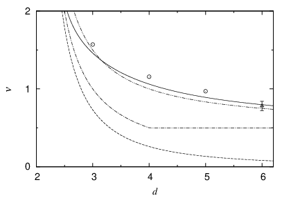
Reference to Table 1 shows immediately that, as expected, the predictions of the self-consistent theory for critical phenomena are not quantitatively accurate. Moreover, the numerical results leave no doubt that the dimensionality dependence of the exponent persists beyond . The prediction that the upper critical dimension is is, therefore, not correct.
Reference to Table 1 and Fig. 5 shows that the predictions of the Borel-Padé analysis of Ref. \citenhikami92 given by Eq. (21) are in poor agreement with the numerical results. The asymptotic behaviour for is clearly incorrect. Moreover, the estimates for higher dimensions violate the well known lower bound[26, 27] for the exponent
| (32) |
According to the semi-classical theory of the Anderson transition presented in Ref. \citengarcia08
| (33) |
The asymptotic behaviour for agrees with Eq. (22). However, the asymptotic behaviour for is only correct at leading order. Nevertheless, reference to Table 1 and Fig. 5 shows that the agreement with the numerical results for and , though certainly not exact, is much better than either the original Borel-Padé analysis Eq. 21 or the self-consistent theory.
Finally, we turn to our new Borel-Padé analysis. Again by reference to Table 1 and Fig. 5 we see that the agreement with the numerical results is slightly worse for but better for and 6 when compared with the semi-classical theory,
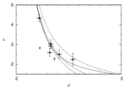
So far we have considered only integer dimensions. Numerical results for the Anderson transition on fractals are also available[17, 36, 18] (See Table 2 and Fig. 6). Fractals are described by several dimensions, among them the spectral dimension. Previous numerical work[17] has established that it is the spectral dimension that determines the universality class. Therefore, we identify with for fractals. The available results allow us to focus on the interval near where the epsilon expansion should be most accurate. (Unfortunately, the authors of Refs. \citenschreiber96 and \citentravenec02 do not agree on the spectral dimension of some fractals.) For sufficiently small both the original and the new Bore-Padé analysis, as well as the self-consistent theory, are in good agrement with the numerical data. The limitations of the semi-classical theory, however, become clearly apparent.
| Eq. (31) | 1 | 0.5 | 0.5 | 0.5 |
|---|---|---|---|---|
| Eq. (21) | ||||
| Eq. (33) | ||||
| Eq. (28) | ||||
| This study | ||||
| ref. \citenslevin14 | ||||
| ref. \citenmarkos06 | ||||
| ref. \citenrodriguez11 | ||||
| ref. \citengarcia07 | ||||
| ref. \citenschreiber96 | ||||
| refs. \citenzharekeshev98 and \citenzharekeshev95 |
| Eq. (28) | ref. \citenschreiber96 | ref. \citentravenec02 | ref. \citensong97 | |
|---|---|---|---|---|
5 Conclusions
We have presented more precise numerical estimates for the critical exponent of the Anderson transition in the and orthogonal universality classes. It may be possible to test these predictions in future experiments on the quantum kicked rotor system in cold atomic gases.
We have also presented a new Borel-Padé analysis, which takes account of the asymptotic behaviour of the exponent as . This new Borel-Padé analysis gives very reasonable agreement with the available numerical estimates of the exponent. The agreement could be improved if either more terms in the -expansion Eq. (19), or alternatively more terms in the asymptotic expansion for beyond the leading order of Eq. (22), were known. Such information could be incorporated in a further revision of the Bore-Padé analysis.
Another possibility would be to incorporate information about the asymptotic behaviour of the coefficients in the -expansion for large order along the lines of Refs. \citenpelissetto02 and \citenguillou77.
Acknowledgements
We would like to thank Michael Schreiber for supplying the numerical data used in Ref. \citenschreiber96. We would also like to thank Tomi Ohtsuki for a critical reading of the manuscript.
Appendix A Asymptotic behaviour for
Here we confirm that the new Borel-Padé analysis has the correct asymptotic behaviour for , i.e., Eq. (19).
The function is said to be asymptotic to the function as if[30]
| (34) |
This is usually written
| (35) |
A series
| (36) |
is said to be asymptotic to the function if[30]
| (37) |
where is the first non-zero coefficient after .
The exponential integral Ei is defined as[40]
| (38) |
and has the following asymptotic expansion for
| (39) |
Using this expansion in Eq.(29) we find for ,
| (40) |
with
| (41) |
For we have explicitly
| (42) |
Eq. (41) is the solution of a three term recurrence relation and we can use this fact to calculate for ,
| (43) |
Using this formula, higher coefficients are more easily calculated,
| (44) |
Upon substitution in to Eq. (28), we find agreement term by term with Eq. (19).
Appendix B Asymptotic behaviour for
Here we demonstrate that the new Borel-Padé analysis has the required asymptotic behaviour for , i.e., Eq. (22).
References
- [1] P. W. Anderson: Phys. Rev. 109 (1958) 1492.
- [2] E. Abrahams, P. W. Anderson, D. C. Licciardello, and T. V. Ramakrishnan: Phys. Rev. Lett. 42 (1979) 673.
- [3] H. Nishimori and G. Ortiz: Elements of phase transitions and critical phenomena (Oxford University Press, New York, 2011).
- [4] F. Evers and A. D. Mirlin: Rev. Mod. Phys. 80 (2008) 1355.
- [5] Y. Harashima and K. Slevin: International Journal of Modern Physics Conference Series 11 (2012) 90.
- [6] I. S. Burmistrov, I. V. Gornyi, and A. D. Mirlin: Phys. Rev. Lett. 111 (2013) 066601.
- [7] M. Amini, V. E. Kravtsov, and M. Müller: New J. Phys. 16 (2014) 015022.
- [8] Y. Harashima and K. Slevin: Phys. Rev. B 89 (2014) 205108.
- [9] F. L. Moore, J. C. Robinson, C. F. Bharucha, B. Sundaram, and M. G. Raizen: Phys. Rev. Lett. 75 (1995) 4598.
- [10] G. Casati, I. Guarneri, and D. L. Shepelyansky: Phys. Rev. Lett. 62 (1989) 345.
- [11] J. Chabe, G. Lemarié, B. Grémaud, D. Delande, P. Szriftgiser, and J. C. Garreau: Phys. Rev. Lett. 101 (2008) 255702.
- [12] M. Lopez, J.-F. Clément, P. Szriftgiser, J. C. Garreau, and D. Delande: Phys. Rev. Lett. 108 (2012) 095701.
- [13] K. Slevin and T. Ohtsuki: Phys. Rev. Lett. 82 (1999) 382.
- [14] K. Slevin and T. Ohtsuki: New J. Phys. 16 (2014) 015012.
- [15] A. Rodriguez, L. J. Vasquez, K. Slevin, and R. A. Römer: Phys. Rev. Lett. 105 (2010) 046403.
- [16] A. Rodriguez, L. J. Vasquez, K. Slevin, and R. A. Römer: Phys. Rev. B 84 (2011) 134209.
- [17] M. Schreiber and H. Grussbach: Phys. Rev. Lett. 76 (1996) 1687.
- [18] I. Travĕnec and P. Markos̆: Phys. Rev. B 65 (2002) 113109.
- [19] A. M. García-García and E. Cuevas: Phys. Rev. B 75 (2007) 174203.
- [20] F. Borgonovi and D. L. Shepelyansky: Physica D 109 (1977) 24.
- [21] D.L.Shepelyansky: arXiv:1102.4450 [cond-mat.dis-nn] .
- [22] F. Wegner: Z. Phys. B 35 (1979) 207.
- [23] L. Schäfer and F. Wegner: Z. Phys. B 38 (1980) 113.
- [24] K. B. Efetov: Adv. Phys. 32 (1983) 53 .
- [25] S. Hikami: Prog. Theor. Phys. Suppl. 107 (1992) 213.
- [26] J. T. Chayes, L. Chayes, D. S. Fisher, and T. Spencer: Phys. Rev. Lett. 57 (1986) 2999.
- [27] B. Kramer: Phys. Rev. B 47 (1993) 9888.
- [28] I. K. Zharekeshev and B. Kramer: Ann. Phys. (Leipzig) 7 (1998) 442.
- [29] P. Markos̆: Acta Phys. slovaca 56 (2006) 561.
- [30] C. M. Bender and S. A. Orszag: Advanced mathematical methods for scientists and engineers (Springer, New York, 1999).
- [31] K. B. Efetov: Physica A 167 (1990) 119.
- [32] A. D. Mirlin and Y. V. Fyodorov: Phys. Rev. Lett. 72 (1994) 526.
- [33] A. M. García-García: Phys. Rev. Lett. 100 (2008) 076404.
- [34] I. M. Suslov: arXiv:1404.7372 [cond-mat.dis-nn] .
- [35] D. Vollhardt and P. Wölfle: in Self-consistent theory of Anderson localization, ed. W. Hanke and Y. V. Kopaev (Elsevier Science Publishers, 1992), p. 40.
- [36] P. H. Song and D. Kim: Phys. Rev. B 55 (1997) 11022.
- [37] I. K. Zharekeshev and B. Kramer: Phys. Rev. B 51 (1995) 17239.
- [38] A. Pelissetto and E. Vicari: Phys. Rept. 368 (2002) 549.
- [39] J. C. Le Guillou and J. Zinn-Justin: Phys. Rev. Lett. 39 (1977) 95.
- [40] A. Jeffrey: Handbook of mathematical formulas and integrals (Elsevier Academic Press, Amsterdam ; Boston, 2004) 3rd ed.