Probing wrong-sign Yukawa couplings at the LHC and a future linear collider
Abstract
We consider the two-Higgs-doublet model as a framework in which to evaluate the viability of scenarios in which the sign of the coupling of the observed Higgs boson to down-type fermions (in particular, -quark pairs) is opposite to that of the Standard Model (SM), while at the same time all other tree-level couplings are close to the SM values. We show that, whereas such a scenario is consistent with current LHC observations, both future running at the LHC and a future linear collider could determine the sign of the Higgs coupling to -quark pairs. Discrimination is possible for two reasons. First, the interference between the -quark and the -quark loop contributions to the coupling changes sign. Second, the charged-Higgs loop contribution to the coupling is large and fairly constant up to the largest charged-Higgs mass allowed by tree-level unitarity bounds when the -quark Yukawa coupling has the opposite sign from that of the SM (the change in sign of the interference terms between the -quark loop and the and loops having negligible impact).
1 Introduction
Now that the existence of a Higgs boson is firmly established [1, 2], the ATLAS and CMS Collaborations at the Large Hadron Collider (LHC) have started probing the Higgs couplings to the fermions and to the gauge bosons [3, 4, 5]. With almost all data from the 8 TeV run analyzed, it becomes increasingly clear that the Standard Model (SM) predictions regarding the Higgs experimental rates are completely consistent with the current experimental data at the 95% C.L., in some cases at the 68% C.L. In the future, the LHC and an International Linear Collider (ILC) could further reinforce this consistency with ever higher precision or could eventually reveal some discrepancies. At this moment in time, it is important to delineate the portions of parameter space of models where qualitative and quantitative differences of the couplings with respect to the SM are consistent with current data but would be revealed by the upcoming LHC runs or at a future collider such as the ILC.
In this work, we will discuss the interesting possibility of a sign change in one of the Higgs Yukawa couplings, for down-type fermions or for up-type fermions, relative to the Higgs coupling to ( or ). It is well known that the current LHC results cannot differentiate between scenarios where a sign change occurs in the Yukawa couplings (see e.g. Refs. [6, 7, 8]) simply using the measured properties of the observed Higgs-like boson and assuming no particles beyond those of the SM. For example, in the most recent fit of Ref. [8], it is found that while the coupling of the Higgs to top quarks must have the conventional positive sign relative to the Higgs coupling to , the couplings of down-type quarks and leptons are only constrained to , where the sign ambiguity arises from the weak dependence of the and loops on the Higgs couplings to bottom-quark pairs. The sign degeneracy in the determination of at the LHC has also been stressed recently in Ref. [9].
In this paper, we will show that the sign of the bottom Yukawa can be determined with sufficient LHC data or at an ILC. The results of this paper will be established in the framework of the softly-broken symmetric (CP-conserving) two-Higgs doublet model (2HDM). The 2HDM possesses two limiting cases (called the decoupling and alignment limits introduced in Section 3), in which the Higgs couplings to , fermion pairs, and the cubic and quartic Higgs self-couplings approach their SM values. But, the 2HDM is also sufficiently flexible as to allow for a SM-like limit for the Higgs couplings to , up-type quark pairs and Higgs self-couplings, but with a coupling to down-type fermions that is opposite in sign to that of the SM. We can thus explore what happens in the context of this specific model when the only tree-level difference relative to the SM is the sign of . The sign of impacts both the and couplings. The coupling will change significantly when the sign of is changed due to the fact that the sign of the interference between the bottom-quark and top-quark loops is reversed. The amplitude is altered primarily because the decoupling of the charged-Higgs loop contribution can be temporarily avoided until a rather large charged-Higgs mass, the boundary being set by the point at which the theory violates tree-level unitarity. Indeed, the nondecoupling of the charged-Higgs loop dominates over the change in the sign of interference terms involving the -quark loop (whose interference is unobservably small on its own), and leads to a potentially observable decrease in the magnitude of the effective coupling. While the change in the sign of interference terms involving the bottom loop is a universal feature that can be used to resolve the relative sign of versus , the charged-Higgs temporary nondecoupling need not be. The latter proves essential in using the final state of Higgs decay to determine the sign of relative to , even allowing said discrimination at the next run of the LHC. Using the coupling is more generically useful and allows the sign determination both at the LHC (albeit somewhat indirectly) and at a future linear collider.
As already implicit in the statements above, it is important to explore the sign issue in the context of a model in which both signs of are allowed and physically distinguishable. The CP-conserving 2HDM provides one such context. Sensitivity to the sign of requires that the measurable collider event rates depend significantly on it. The collider event rates are conveniently encoded in the cross section ratios defined by
| (1.1) |
where is the Higgs production cross section and is the branching ratio of the decay to some given final state ; and are the expected values for the same quantities in the SM. The experimentally measured values of for a variety of final states at the LHC already provide interesting constraints on the 2HDM parameter space [10].
In this paper, we do not separate different LHC initial state production mechanisms (, , , associated production and associated production); that is, we sum over all production mechanisms in computing the cross section. In our analysis of Higgs phenomena at the ILC, we consider only the production process. We employ the notation when discussing these ratios for the LHC and ILC, respectively. In deciding whether or not a given 2HDM parameter choice is excluded by LHC data for given values of , all the currently well-measured final states must be employed. In particular, we will find that is only consistent with current LHC Higgs data for a 2HDM of type-II if the deviations in the and/or couplings will be detectable in the future with the LHC operating at , assuming an accumulation of luminosity , and at a future ILC.
This paper is organized as follows. In Section 2, we describe the 2HDM and the constraints imposed by theoretical and phenomenological considerations. In Section 3 we introduce the decoupling and alignment limits, and then define the wrong-sign Yukawa couplings scenario and discuss its properties. In Section 4 we analyze the detailed phenomenology of the wrong-sign Yukawa coupling scenario, and in Section 5, we exhibit the results of our analysis. Our conclusions are presented in Section 6. Appendix A provides details regarding the Higgs basis scalar potential parameters of the 2HDM relevant for Section 3. The Higgs sector of the minimal supersymmetric extension of the Standard Model (MSSM) [11] is a special case of the type-II 2HDM introduced in Section 2. The possibility of an MSSM Higgs sector with an opposite-sign coupling relative to the SM is addressed in Appendix B. Finally, Appendix C explains the nondecoupling behavior of the charged-Higgs loop contribution to the amplitude in a type-II 2HDM that is particularly relevant when has a sign opposite that of the SM.
2 Models and constraints
The 2HDM is an extension of the scalar sector of the SM with an extra hypercharge-one scalar doublet field, first introduced in Ref. [12] as a means to explain matter-antimatter asymmetry (see Refs. [13, 14] for a detailed description of the model). The most general Yukawa Lagrangian, in terms of the quark mass-eigenstate fields, is:
| (2.1) |
where and is the CKM mixing matrix. In eq. (2.1) there is an implicit sum over the index , and the are Yukawa coupling matrices. In general, such models give rise to couplings corresponding to tree-level Higgs-mediated flavor-changing neutral currents (FCNCs), in clear disagreement with experimental data.
A natural way to avoid FCNC interactions is to impose a symmetry on the dimension-four terms of the Higgs Lagrangian in order to set two of the equal to zero in eq. (2.1) [15]. This in turn implies that one of the two Higgs fields is odd under the symmetry. The Higgs potential can thus be written as:
| (2.2) | |||||
where softly breaks the symmetry. In particular, we do not allow a hard breaking of the symmetry, which implies that the term of the form is absent. For simplicity we will work with a CP-conserving scalar potential by choosing and to be real.
The 2HDM parameters are chosen such that electric charge is conserved while neutral Higgs fields acquire real vacuum expectation values,11 1 A sufficient condition for guaranteeing that the vacuum is CP invariant is (see e.g. Appendix B of Ref. [16]). Moreover, the existence of a tree-level scalar potential minimum that breaks the electroweak symmetry but preserves both the electric charge and CP symmetries, ensures that no additional tree-level potential minima that spontaneously break the electric charge and/or CP symmetry can exist [17]. As such, in our simulations we can be certain that and can be chosen real. (for ), where
| (2.3) |
By convention, we take (after a suitable rephasing of the Higgs doublet fields). From the 8 degrees of freedom we end up with three Goldstone bosons, a charged-Higgs pair, two CP-even neutral Higgs states, and (defined such that ), and one CP-odd neutral Higgs boson . The CP-even Higgs squared-mass matrix is diagonalized by an angle , which is defined modulo . The coupling of to is specified by
| (2.4) |
As noted above, Higgs-mediated tree-level FCNCs can be avoided by imposing a symmetry that is preserved by all dimension-four interactions of the Higgs Lagrangian. Different choices for the transformation of the fermion fields under this lead to different Higgs-fermion interactions. In this paper, we shall focus on two different choices, which lead to models that are called the type-I [18, 19] and type-II [20, 19] 2HDM. In the type-I 2HDM, in eq. (2.1), whereas in the type-II 2HDM, . In the former all fermions couple exclusively to while in the latter the up-type quarks couple exclusively to and the down-type quarks and charged leptons couple exclusively to . In both the type-I and type-II 2HDM, the Higgs-fermion couplings are flavor diagonal and depend on the two angles and as shown in Table 1. The tree-level MSSM Higgs sector is a special case of the type-II 2HDM [11].
| Type-I | Type-II | |||||||||||||
|---|---|---|---|---|---|---|---|---|---|---|---|---|---|---|
| Up-type quarks | ||||||||||||||
| Down-type quarks and charged leptons | ||||||||||||||
The most relevant constraints on the 2HDM are briefly discussed in Ref. [21]. Here, we will just enumerate the constraints imposed on the parameters of the CP-conserving 2HDM.
Finally we should note that there is an unexplained discrepancy between the value of measured by the BaBar collaboration [40] and the corresponding SM prediction. The observed deviation is of the order 3.4 . If confirmed, this observation would exclude both the SM and the version of the 2HDM considered in this work.
3 Decoupling, alignment, delayed decoupling and the wrong-sign Yukawa couplings
In light of the fact that the LHC Higgs data is consistent with the predictions of the Standard Model with one complex hypercharge-one Higgs doublet, it is of interest to consider the limit of the 2HDM in which the properties of the lightest CP-even Higgs boson approach those of the SM Higgs boson. It is convenient in this section to adopt a sign convention in which is non-negative,22 2 The implications of an alternative convention , employed in the 2HDM parameter scans of Sections 4 and 5, will be addressed later in this section. i.e. . Since
| (3.1) |
it follows that is SM-like in the limit of .
It is convenient to rewrite the Higgs potential of eq. (2.2) in terms of new scalar doublet fields defined in the Higgs basis [41, 42, 43, 44, 45, 46, 47]. The coefficients of the quartic terms of the scalar potential in the Higgs basis are denoted by (where ). Expressions for the in terms of the defined by eqs. (A.6)–(A.10) are given in Appendix A. In particular, using eqs. (A.6) and (A.9), it follows that,
| (3.2) | |||||
| (3.3) |
By assumption, the sizes of the scalar potential parameters (in any basis) are limited by tree-level unitarity constraints. This means that and . It follows that if then in which case has SM-like couplings to . This is the decoupling limit [48, 16], where and [i.e. ], and the couplings approach those of the Standard Model. That is, below the common scale of the heavy Higgs states, the effective field theory that describes Higgs physics is the Standard Model with a single hypercharge-one Higgs doublet. However, note that if is SM-like, it does not necessarily follow that the masses of , and are large. Indeed, eq. (3.3) implies that it is possible to achieve by taking [49, 16]. The limit where is called the alignment limit [50, 51, 52, 53], since in this limit the mixing of the two-Higgs-doublet fields in the Higgs basis is suppressed.33 3 In the alignment limit where , it is possible to have , in which case we would identify the heavier CP-even state as the SM-like Higgs boson. We will not consider this possibility further in this paper.
In both the decoupling and alignment limits, the couplings of to the fermions should also approach their SM values. To see how this happens, consider the couplings in the case of the type-II 2HDM. Using the results displayed in Table 1, the couplings relative to those of the SM (for ) are given by:
| (3.4) | |||||
| (3.5) |
In the case of , the couplings reduce precisely to the corresponding SM values. However, for values of that are small but nonzero, the decoupling limit can be “delayed” if either or is large. On the other hand, it is desirable to have and , in order to avoid nonperturbative behavior in the couplings of , and to the third generation at scales far below the Planck scale. In addition, phenomenological constraints arising from physics observables and mentioned above rule out regions of for large regions of the 2HDM parameter space [31]. Consequently, we shall focus on the parameter region where
| (3.6) |
In this case, decoupling is not delayed for the coupling of to up-type fermions. On the other hand, for in the range of interest, it is certainly possible to have close to 1 and yet have significant departures from decoupling in the coupling of to down-type fermions. That is, it is possible to have close to 1 and yet have . Since behaves as in the decoupling limit [cf. eq. (3.3)], we see that the coupling approaches its SM value if
| (3.7) |
Thus, if we say that we have delayed decoupling [54], since a much larger value of the heavy Higgs mass scale is required to achieve decoupling of the heavy Higgs states (i.e. is not sufficient).44 4 Likewise, the alignment limit is also delayed, since the condition is now replaced by .
The wrong-sign Yukawa coupling regime is defined as the region of 2HDM parameter space in which at least one of the couplings of to down-type and up-type fermion pairs is opposite in sign to the corresponding coupling of to . This is to be contrasted with the Standard Model, where the couplings of to and are of the same sign. Note that in the convention where , the couplings in the 2HDM are always non-negative. To analyze the wrong-sign coupling regime, it is more convenient to rewrite the type-II Higgs-fermion Yukawa couplings, given by eqs. (3.4) and (3.5), in the following form:
| (3.8) | |||||
| (3.9) |
In the case of , the coupling normalized to its SM value is equal to (whereas the normalized coupling is ). Note that in this limiting case, , which implies that the wrong-sign Yukawa coupling can only be achieved for values of . Likewise, in the case of , the coupling normalized to its SM value is equal to (whereas the normalized coupling is ). In this limiting case, , which implies that the wrong-sign couplings can only be achieved for . In the type-I 2HDM, both the and couplings are given by eq. (3.5) [or equivalently by eq. (3.9)]. Thus, for , both the normalized and couplings are equal to , which is only possible if . In light of eq. (3.6), only the wrong-sign coupling regime of the type-II 2HDM can be realistically achieved.
It should be emphasized that the above conclusions do not depend on the convention adopted for the range of the angle . In the convention used in Sections 4 and 5 of this paper, we scan over , which allows for the possibility of negative . However, the definition of the wrong-sign Yukawa coupling is not changed as it refers to the relative sign of the and couplings. To translate between both conventions, one simply must shift (the sign chosen so that is in its desired range). In practice, the scans of Section 4 and 5 focus on the wrong-sign coupling regime where , in which case and the distinction between the two conventions becomes moot.
In the above discussion of the wrong-sign Yukawa coupling regime, we have not yet imposed the requirement that is SM-like. In particular, for a fixed value of , the limit of is not the decoupling limit (indeed the couplings do not approach their SM values except in the limit of and ). This implies that for we must have , Likewise, the limit of is not the decoupling limit unless and , i.e. . Again, we see that for values of , among all possible wrong-sign Yukawa coupling scenarios only the wrong-sign coupling in the type-II 2HDM is phenomenologically viable.
Therefore, in this paper, we shall explore the possibility that the coupling normalized to its SM value is close to in the type-II 2HDM.55 5 The possibility that a parameter regime of the MSSM Higgs sector exists with a wrong-sign coupling is addressed in Appendix B. This scenario was first examined in Ref. [55] and then later clarified in Ref. [16]. Current LHC Higgs observations are not sufficiently precise as to allow one to distinguish this case from that of the SM Higgs boson. To study this case, we first define a parameter by defining the normalized coupling to be given by
| (3.10) |
Multiplying eq. (3.10) by , and employing the trigonometric identity, , it follows that66 6 Although we are interested in the 2HDM parameter regime where is small, eq. (3.11) is valid for all values of . In particular, for we have and , which is consistent with the result of eq. (3.11).
| (3.11) |
By employing the trigonometric identity and taking , one can also derive
| (3.12) | |||||
| (3.13) |
Using eqs. (3.4) and (3.10), it follows that
| (3.14) |
Since the couplings are assumed to be close to the SM, we still must impose the constraint that . Thus, in the case of the wrong-sign Yukawa coupling, we must have , which is the region of delayed decoupling defined below eq. (3.7).
For completeness, we also also examine the case of a wrong-sign coupling in the type-II 2HDM (or the case of the wrong-sign and couplings in the type-I 2HDM) by taking close to [cf. eq. (3.9)]. To study this case, we first define a parameter via
| (3.15) |
which yields an coupling normalized to its SM value given by . An analysis similar to the one used in the case of the wrong-sign Yukawa coupling yields
| (3.16) |
and
| (3.17) | |||||
| (3.18) |
Using eqs. (3.5) and (3.14), it follows that
| (3.19) |
For values of , eq. (3.19) can only be satisfied if , which lies outside the range of under consideration [cf. eq. (3.6)], as previously noted.
To complete the analysis of the tree-level Higgs couplings, we briefly look at the self-coupling. In the 2HDM, the coupling77 7 A similar analysis can be given for the coupling using the results given in Ref. [16]. However, this coupling cannot be realistically probed by the LHC and ILC, so we will not provide the explicit expressions here. is given by [16]:
| (3.20) |
where in the softly broken symmetric 2HDM, the are given in eqs. (A.6)–(A.10). Rewriting the in terms of the yields
| (3.21) |
which reproduces the result given in Ref. [56]. Using the results of Appendix D of Ref. [16], we can rewrite the coupling in a more convenient form,
| (3.22) |
which reproduces the result given in Ref. [57] (after correcting a missing factor of 2).
In the decoupling/alignment limit where , we have and . Then, the coupling reduces to the SM value,
| (3.23) |
In the wrong-sign Yukawa coupling limit for type-II Higgs couplings to down-type [up-type] fermions, respectively, where [], we have and , so that
| (3.24) |
which reduces to the SM value only when [] for type-II Higgs couplings to down-type [up-type] fermions, respectively. It is quite remarkable that this matches the behavior of the coupling in the same limit. In particular, for , we have , as previously noted. Hence in the wrong-sign Yukawa coupling limit, eq. (3.1) yields
| (3.25) |
Of course, the corresponding first order corrections to the and couplings will differ as one moves away from the strict limiting case treated above.
In the decoupling and alignment limits discussed at the beginning of this subsection, the tree level couplings of approach the corresponding values of the SM Higgs boson. The behavior of the decoupling and alignment limits differ when one-loop effects are taken into account. In the decoupling limit, the properties of continue to mimic those of the SM-like Higgs boson since the effects of the , and loops decouple in the limit of heavy scalar masses. In contrast, the alignment limit only requires that , so that in principle the masses of , and could be relatively close to the electroweak scale. In this case, the loop effects mediated by , and can compete with other electroweak radiative effects and thus distinguish between and the SM Higgs boson.
In processes in which the one-loop effects are small corrections to tree level results, very precise measurements will be required to distinguish between and the SM Higgs boson in the alignment limit. Indeed, a much more fruitful experimental approach in this case is to search directly for the , and scalars! However, in Higgs processes that are absent at tree level but arise at one-loop, the loop effects mediated by , or can compete directly with deviations that arise due to small departures from the alignment limit. The most prominent example is the decay rate for . Departures from the SM decay rate for can arise either from deviations in the , and/or couplings from their SM values, or from the contributions of the charged-Higgs boson loop (which is not present in the SM). To compute the latter, we need to compute the coupling. Using the results of Ref. [16],
| (3.26) |
where and are defined in terms of the in eqs. (A.8) and (A.10). It is convenient to reexpress the coupling in terms of the Higgs masses and . Using the expressions given in Appendix D of Ref. [16], we obtain
| (3.27) |
where
| (3.28) |
In the alignment limit where the masses of , and are of order the electroweak scale, and the charged-Higgs loops can compete with the SM loops that contribute to the one-loop amplitude. In the normal decoupling limit where and , as expected, in which case the charged-Higgs loop contribution to the amplitude is suppressed by a factor of . Note that this factor is of the same order as . The contribution of the fermion loops also deviates from the SM by a factor of due to the modified tree level couplings [cf. eqs. (3.4) and (3.5)].88 8 The contribution of the loop deviates from the SM by a factor of in light of eq. (3.1). However, in the decoupling limit the contribution of the bottom-quark loop is suppressed by a factor of and can thus be ignored. We conclude that the deviation from the SM in the decoupling limit is due primarily to the top-quark loop and the charged-Higgs loop, whose contributions to the decay amplitude are of the same order of magnitude.
The form of the coupling given in eq. (3.27) suggests the existence of 2HDM parameter regimes in which , even under the assumption that . For example, if we allow to be large and if , , , then it possible to have . It would then follow that the contribution of the charged-Higgs loop contribution to the amplitude, which scales as , approaches a constant in the region of . This nondecoupling behavior was first emphasized in Ref. [58] and subsequently reexamined in Ref. [59]. Indeed, the behavior of the charged-Higgs loop in the nondecoupling regime is similar to the contribution of a heavy fermion loop to the amplitude, which scales as and approaches a constant for . In particular, if is too large, then and tree level unitarity is violated. However, there is an intermediate range of heavy fermion masses above but below the mass scale at which tree level unitarity is violated, in which the fermion loop contribution to the amplitude is approximately constant. Likewise, if is too large then one would need to take above its unitarity bound [in light of eq. (3.26)]. Again, there is an intermediate region of heavy Higgs masses (where tree level unitarity is still maintained) in which the charged-Higgs loop contribution to the amplitude is approximately constant. Thus, we expect regions of 2HDM parameter space in which a SM-like Higgs can exhibit a non-negligible deviation in from SM expectations.
Alternatively, the second term on the right-hand side of eq. (3.27) can be enhanced in the delayed decoupling regime where and . In this case, [under the assumption that , ]. However, this behavior is also associated with growing quartic couplings that can potentially violate tree level unitarity. Indeed, by comparing with eq. (3.26), we see that is being enhanced. More directly, it is straightforward to obtain
| (3.29) |
which again implies that some of the Higgs potential parameters must be enhanced by a factor of if and . Thus, if becomes too large, the unitarity constraints on the Higgs potential quartic coupling parameters will be violated. Nevertheless, there exists an intermediate range of charged-Higgs masses in which tree level unitarity is maintained while the charged-Higgs loop contribution to the amplitude is approximately constant. That is, there exists a region of 2HDM parameter space, in which is small and the coupling is opposite in sign to that of the SM Higgs boson, where a deviation in the decay rate from the predicted SM rate due to the contribution of the charged-Higgs loop can be detected.
Details on the nondecoupling of the loop contribution to the amplitude can be found in Appendix C, where it is shown that such nondecoupling is inevitable for the wrong-sign coupling scenario. The resulting magnitude of the effect yields deviations from the SM that will ultimately be observable at the LHC and a future linear collider, as discussed in the following sections.
4 Phenomenology of the Wrong-sign Yukawa couplings
It is convenient to define the ratio of the coupling to the corresponding SM value as
| (4.1) |
where we will be considering , , , , . As for the coupling to photons, is defined as
| (4.2) |
with an analogous definition for . Note that and are strictly positive, whereas the remaining could be either positive or negative. These definitions for the couplings coincide with the definitions used by the experimental groups at the LHC [60], at leading order. We shall also make the simplifying assumption (which holds in the SM and in the 2HDM under consideration) that all down-type [up-type] fermion final states are governed by the same []. It is convenient to begin with a simplified discussion of the impact of changing the sign of in order to set the stage. In this section, we employ the convention of for which in both type-I and type-II models. For this choice, the coupling of eq. (2.4) can, in principle, be either positive or negative. However, for , the phenomenology of the final state requires that the coupling be positive, which means that acceptable regions of parameter space must have .
Consider first the amplitude of the process . In an appropriate normalization, the top- and bottom-quark loops contribute and , respectively, when and . This implies a large fractional change in the coupling with a change of sign of . One finds a shift in of in going from positive to . Naively, one would suppose that this large shift would be easily observed. However, this is a difficult task at the LHC due to the challenge in identifying gluons (even if indirectly) in the final state. In addition, the primary fusion production cross section has some systematic errors associated with higher order corrections. Nonetheless, Table 1-20 of Ref. [61] gives expected errors for of – for and – for , based on fitting all the rates rather than directly observing the final state. At the ILC, the primary production mechanism of is very well determined in terms of the coupling and isolation of the final state is easier. The error on estimated in Ref. [61] is for a combination of at and at . Other error estimates are to be found in Ref. [62, 51] where it is concluded that can be measured at the ILC with an accuracy of 8.5% at a center-of-mass (CM) energy of 250 GeV and 7.3% at a CM energy of 350 GeV with an integrated luminosity of 250 fb-1 and beam polarization of 80% (electron) and 30% (positron) [62]. The error estimate for with decreases to (see Tables 6.1 and 6.2 of Ref. [51]), consistent with the estimate from Ref. [61]. Thus, in the end, we can anticipate that both the LHC and ILC will be able to determine whether or not is positive using the indirect fit and direct measurement of , respectively.
In , the presence of the large -boson loop contribution means that considerable precision is required to identify the interference effects. In more detail, the contributions to the amplitude of this process assuming SM couplings are as follows [these are the ’s defined in eq. (C.5)]; boson, ; top-quark loop (with ), ; bottom loop for , . As a result, switching the sign of would change from to , i.e. a shift. The accuracy with which can be measured at the 14 TeV LHC is given in Table 1-20 of Ref. [61] as – for integrated luminosity of and – for . The ranges correspond to optimistic/pessimistic estimates regarding systematic and theoretical errors. Thus, if the change in was only of order this could not be detected at the LHC. Nonetheless, we claim that with high enough integrated luminosity one can distinguish from in the context of the type-II 2HDM using the high precision final state due to the fact that the coupling is inevitably suppressed in the case as a result of a large nondecoupling charged-Higgs loop contribution, i.e. one that approaches a constant at large charged-Higgs mass (up to the limit at which the couplings violate the tree level unitarity bounds). There is also a region of parameter space for which the charged-Higgs loop does not decouple, and this region would be ruled out in very similar fashion to the region we focus on. In fact, the modification to the coupling is the only way of revealing this nondecoupling region. However, for there is also the standard decoupling region for which the charged-Higgs loop does decouple and that would allow arbitrarily precise agreement with the SM predictions. A detailed discussion of nondecoupling and perturbativity/unitarity bounds is given in Appendix C. Typically, is inevitably suppressed relative to the SM prediction by about 5% for , which should be measurable at the LHC run for . At the ILC, for a combination of at and at the expected error on is (including a theory uncertainty) based on measuring with , implying that the sign of cannot be directly determined at the ILC using the final state.
To explore in more detail, we scan over the 2HDM parameter space subject to all the constraints described in section 2. We begin by fixing . The charged-Higgs mass is varied between 100 and 900 GeV in type-I and 340 and 900 GeV in type-II. The heavier CP-even scalar mass was kept between 125 and 900 GeV while the pseudo-scalar mass range is between 90 and 900 GeV. The soft-breaking parameter was varied in the range while . After passing all constraints, the points were used to calculate the various , which is the ratio of the number of events predicted by the model for the process to the SM prediction for the same final state,
| (4.3) |
In computing the cross section, we have summed over all light Higgs production mechanisms ( fusion, fusion, associated production, fusion, and associated production),99 9 Further discrimination among models and parameter choices within a model can be obtained by separately considering each individual initial state final state combination, as is now done by the LHC experimental collaborations and considered in Ref. [8]. employing a mass of . The processes that involve only Higgs couplings to gauge bosons can be obtained by simply rescaling the SM cross sections. Hence, for Higgs Strahlung and vector boson fusion we have used the results of Ref. [63] (the same applies to the final state ). We have included QCD corrections but not the SM electroweak corrections because they can be quite different for the 2HDMs. Cross sections for are included at next-to-next-to-leading order (NNLO) [64] and the gluon fusion process was calculated using HIGLU [65]. (When the Higgs boson is SM-like, the cross section is much smaller than the cross section.) Our baseline will be to require that the for final states , , , and are each consistent with unity within 20%, which is a rough approximation to the precision of current data. We then examine the consequences of requiring that all the be within 10% or 5% of the SM prediction. This enables us to understand how an increase in precision affects the scenario we will now describe in detail.


As discussed in Sections 2 and 3, the relative coupling is given by . The relative Higgs-fermion couplings are in the type-I 2HDM, whereas in the type-II 2HDM,
| (4.4) |
In Fig. 1 we show in type-I and type-II models as a function of for those parameter space points that pass all theoretical and experimental constraints and have all within 20% of the SM prediction of 1. In all cases, , which implies that a wrong-sign Yukawa coupling would correspond to a negative value of or . Noting that in the convention of , it follows that only regions with correspond to a wrong-sign Yukawa coupling scenario.
As expected, the left panel of Fig. 1 shows that all points are very close to for a type-I 2HDM, while the right panel shows that in the case of the type-II 2HDM all points fall within two main regions: one where and the other one where . In short, although the LHC results have clearly shown that the Higgs rates to fermions and gauge bosons are very consistent with the SM predictions, it is clear that the roughly precision with which LHC rates are currently measured allows for a second non-SM-like region with the opposite sign of that can fit within the context of the type-II 2HDM.
In Section 3, we showed that in the type-II 2HDM, the region corresponds to the limit whereas the region is attained in the limit ,
| (4.5) |
corresponding to negative and positive values of , respectively (in a convention where ). On the other hand, the relative and couplings satisfy
| (4.6) |


In Fig. 2, the left panel shows as a function of with all within 20% (blue/black), 10% (green/light grey) and 5% (red/dark grey) of their SM values. We clearly see two branches—one with corresponding to the SM limit and one with corresponding to the wrong-sign Yukawa coupling scenario. In the left branch, the points are all such that ; the points in the right branch all have . The right panel shows that as increases the branch corresponds to parameters with small , i.e. . Note that the second branch is excluded if we demand that all the fall within 5% of unity.
It is instructive to consider why with is still allowed by current data. Note that eq. (3.11) implies that at very large where ,
| (4.7) |
In particular, when we see that is always below . Fig. 2 reflects the behavior shown in eq. (4.7) in that the larger is, the closer the negative and positive regions are. Furthermore, as decreases the region where the low values of are allowed decreases. Therefore, when is very large we see that , and we recover the SM and couplings. Furthermore, as discussed earlier there is limited sensitivity to the sign of the Yukawa couplings for the one-loop induced and couplings. Thus, due to the limited accuracy with which the and couplings are (indirectly) measured, the region of wrong-sign Yukawa couplings (where and ) in the type-II 2HDM is still allowed by the current LHC data.
5 Results and discussion
In order to study in more detail the wrong-sign region of the type-II 2HDM, we have generated a new set of points where we have further imposed that . In the left panel of Fig. 3 we present as a function of , with all within 20% of the SM values in blue (black) and 10% of the SM values in green (light grey). As expected, the values are very close to the region where while simultaneously approaches 1. As the values are required to agree more precisely with the SM value of 1, the points move closer to the above limit. In the right panel we show the same ratio as a function of . As grows, is forced to be closer to as indicated in eq. (4.7) and is forced to be closer to 1 due to the LHC constraints. As indicated by Fig. 2, increasing the precision of the Higgs measurements would allow exclusion of the low region if all are within 10% of unity. Moreover, the entire region is eliminated if all are within 5% of unity.


In fact, we will see that it is that makes overall consistency with SM rates at the 5% level impossible in the branch. This is due to the fact that for all the points we are in the nondecoupling regime for which the charged-Higgs boson loop contribution to the amplitude is approximately constant as a function of (up until the tree level unitarity upper limit of , beyond which is not a perturbatively consistent possibility). The charged-Higgs loop gives about a reduction in that is inconsistent with being within of unity. The details of the nondecoupling regime are discussed at length in Appendix C.
Another perspective is obtained by examining Fig. 4. There, we have shown regions in vs. space where either (cyan/grey) or (black) are within of unity for points in the branch.1010 10 Note that in the 2HDM, implying that measurements in the channel are equally useful. Further, at the LHC, the final state will be more precisely measured than for the final state. We observe that the two branches represented do not intersect, and as such it is impossible to achieve 5% agreement with the SM in both of these channels. This explains why there are no red points in the right branch of the plots in Fig. 2.
Further insight is gained from Fig. 5, which considers points for which the are within 5% of the SM value of 1. On the left, we exhibit the values of and vs . This shows that while can be within 5% of unity, cannot — it is always more than 7-8% below unity, implying that 5% accuracy on this channel would exclude the branch. On the right, we plot vs. . The largest value of that can be achieved is , and this only if . Thus, it is the suppression of the final state at the LHC that is key to ruling out the possibility for operation at high luminosity. This same conclusion is found in the work of Ref. [66]. There, different initial states are separated from one another and one finds that the rate is the most suppressed relative to other processes — because of the 6% enhancement of when the rate is not as suppressed relative to the remaining processes but still contributes to the overall inconsistency for between these final state channels with other final states such as , and when all are measured with 5% accuracy.


In Fig. 6, we show in or vs. space the points that are allowed if the ’s are each within (blue), (green), or (red) of unity (the SM limit). We observe from the left hand plot that is always at least 5% below unity in the region and that accuracy on the ’s will eliminate this region entirely. In fact, as we saw in Fig. 5 it is that necessarily has a greater than deviation from unity. The right hand plot shows that in the region, is always bigger than 1.13. However, since currently the LHC is unable to determine with the necessary accuracy this does not help to exclude the region. But, as summarized earlier, with at , can be determined to about accuracy and such a deviation will certainly be observable.
As noted earlier, at the ILC the final state becomes a powerful tool for determining the sign of . Thus, we shall explore the final state issues in more detail. In Fig. 7 we exhibit as a function of for (left) and (right) with all within 20% of the SM values in blue (dark grey) and 10% of the SM values in green (light grey). Contrary to the SM-like scenario, when (wrong-sign Yukawa coupling) the value of the ratio of the widths is always above 1.25. Fig. 7 shows that the minimum value of becomes larger when smaller deviations of the s from unity are required. In particular, when the coupling changes sign but all tree level couplings have SM magnitude, the ratio between the two widths is exactly
| (5.1) |
which is in agreement with HDECAY [67, 68] and 2HDMC[69, 68]. Note that this interference effect, which is almost 30% relative to the SM, does not manifest itself in the production process that is important for the LHC and might therefore have been quite easily detectable. In contrast to the leading order (LO) result,
| (5.2) |
at NNLO in the limit of , [65] while the ratio of the partial widths of does not suffer any significant change in going from LO to NNLO. Therefore, the present LHC data cannot discriminate between the two scenarios based on interference effects at the production level; it is only through a luminosity of data accumulated at and a combined fit of the rates for all final states that one can manage to determine the underlying with adequate precision.


Of course the ILC can probe more easily and directly using the process . We define
| (5.3) |
where is the measured Higgs production cross section at the ILC and and are the SM values of the production cross section at the ILC and branching ratio of a Higgs decaying to a pair of gluons. The ratio of the cross sections in the process is just . Likewise we can define similar ratios for the processes and which we will call and , respectively.


In the left panel of Fig. 8 we show the quantity as a function of . When all ’s measured at the LHC are forced to be within 20% of the SM values (blue/black) all points are above 1.12. If the precision is increased to 10%, the bound is increased to 1.25. Recently, it was shown that can be measured at the ILC with an accuracy of 8.5% at a CM energy of 250 GeV and 7.3% at a CM energy of 350 GeV with an integrated luminosity of 250 fb-1 and beam polarization of 80% (electron) and 30% (positron) [62, 51]. The 95% C.L. predicted measurement for GeV and 250 fb-1 luminosity is 1.02 0.07 [62], assuming SM expectations. Therefore, this measurement could exclude all points in the left panel of Fig. 8. In the right panel we present as a function of . The corresponding SM predicted measurement for the ILC is 1.00 0.01. Clearly, a better than about measurement of can also help probe the wrong-sign coupling provided enough precision is attained at the LHC in the measurements of the Higgs couplings to fermions and gauge bosons. The values of are slightly below 1 because, as can be seen from eq. (4.7), when , is slightly below 1 as the right-hand side of the equation is positive. Note that the ratio of the branching ratios in is very close to 1 in the limit we are considering and as such . Similar results would be obtained for , where the final state is , but the precision in the measurement is not as good as for .
6 Conclusions
The couplings of the Higgs boson recently discovered at the LHC to the fermions and gauge bosons are starting to be measured with some precision. It is important to understand the implications of these results in the context of specific Higgs sector models. In this paper, we considered type-I and type-II -symmetric and CP-conserving 2HDMs. Our focus was on the fact that the sign of the Yukawa coupling to the down-type fermions could be opposite to that of the SM. Using scans over type-I and type-II parameter spaces, subject to basic theoretical and experimental constraints as described in the main text, we found that a sign change in the down-quark Yukawa couplings can be accommodated in the context of the current LHC data set at 95% C.L., but only in the case of the type-II 2HDM when . The situation is different in the type-I 2HDM — because only one doublet couples to all fermions the sign change would result in deviations from the SM predictions that are incompatible with the current Higgs data set. In this paper, we address the possibility of probing the wrong-sign Yukawa coupling of the Higgs to down-type quarks with future measurements of Higgs properties at the LHC and at the International Linear Collider.
In particular, we performed a scan dedicated to the part of type-II 2HDM parameter space where the wrong-sign down-type quark coupling is currently acceptable. We filtered parameter space points requiring that the values of , the production rate of a given final state relative to the SM, are within either 20%, 10% or 5% of the SM predictions for the LHC. Of greatest immediate interest is the fact that projected precisions for the determination of the magnitude of the coupling relative to its SM value, (using in particular) imply that the LHC with and will either rule out or confirm the wrong-sign scenario. Of particular importance for this conclusion is the fact that the charged-Higgs loop contribution to the couplings does not decouple for the scenario, leading to a decrease in . This statement applies for any charged-Higgs mass below the bound of about for which the Higgs coupling parameters satisfy tree level unitarity bounds. In the context of the model, a finding that the Yukawa has a negative sign and also detecting a charged-Higgs with mass above would imply that the theory is in a realm where perturbative calculations become suspect.
In addition, we have shown that the predictions for the measurements of and at the ILC would allow us to probe the wrong-sign Yukawa coupling of a type-II 2HDM. Therefore, at both collider facilities, either a measurement or a definite 95% exclusion limit could be set on the wrong-sign Yukawa coupling scenario.
Acknowledgements.
The works of P.M.F. and R.S. are supported in part by the Portuguese Fundação para a Ciência e a Tecnologia (FCT) under contract PTDC/FIS/117951/2010, by FP7 Reintegration Grant, number PERG08-GA-2010-277025, and by PEst-OE/FIS/UI0618/2011. The work of J.F.G. and H.E.H. is supported in part by the U.S. Department of Energy, under grant numbers DE-SC-000999 and DE-FG02-04ER41268, respectively. J.F.G. and H.E.H. also thank the Aspen Center for Physics, supported by the National Science Foundation under grant number PHYS-1066293, for hospitality and a great working atmosphere. J.F.G. acknowledges conversations and related collaboration with B. Dumont, Y. Jiang and S. Kraml. R.S. acknowledges discussions with M. Mühlleitner, M. Spira and J.P. Silva. Finally, H.E.H. is grateful for probing questions by JoAnne Hewett, which inspired the inclusion of Appendix B.Appendix A The Higgs basis of the softly broken symmetric CP-conserving 2HDM
It is convenient to reexpress the Higgs potential given by eq. (2.2) in the Higgs basis [41, 42, 43, 44, 45, 46, 47]. By assumption, we have assumed that all the scalar potential parameters and the two vacuum expectation values and are real, which implies that the scalar potential and the vacuum are CP invariant. By a suitable transformation on the two-Higgs-doublet fields (), one can define two new linearly independent Higgs doublet fields and such that and . This is accomplished by defining
| (A.1) |
The Higgs basis is uniquely defined up to an overall sign of the scalar doublet field. In the Higgs basis, the scalar potential is given by
| (A.2) | |||||
where the squared-mass terms are given by:
| (A.3) | |||||
| (A.4) | |||||
| (A.5) |
and the Higgs basis quartic couplings are given by
| (A.6) | |||||
| (A.7) | |||||
| (A.8) | |||||
| (A.9) | |||||
| (A.10) |
Note that one is free to redefine , and by an overall sign in light of the sign ambiguity in defining the Higgs basis. The potential minimum conditions are especially simple in the Higgs basis,
| (A.11) |
leaving as the only free squared-mass parameter of the model.
Appendix B The wrong-sign coupling and the MSSM Higgs sector
The tree level scalar potential of the MSSM Higgs sector is given by eq. (2.2), with [11]
| (B.1) |
In particular [defined below eq. (2.2)]. Inserting eq. (B.1) into eqs. (A.6)–(A.10) yields [70]
| (B.2) |
Using the result for given above in eqs. (3.2) and (3.3) yields the tree level expressions,
| (B.3) | |||||
| (B.4) |
where are the MSSM tree level CP-even Higgs squared masses,
| (B.5) |
In addition, the MSSM tree level Higgs-fermion Yukawa couplings possess a type-II structure due to supersymmetry.
In the decoupling limit where , eq. (B.3) implies that (in the convention where ). Using eq. (B.4),
| (B.6) |
for all values of . In particular, for , one can never have in the decoupling regime. Thus, in the tree level Higgs sector of the MSSM, the phenomenon of delayed decoupling discussed below eq. (3.7) does not occur. In light of eq. (3.4), one cannot achieve the wrong-sign Yukawa coupling in the region of the tree level MSSM Higgs sector parameter space where the coupling is SM-like.
It is well known that radiative corrections can significantly alter the properties of the MSSM Higgs sector (reviewed in, e.g., Refs. [71] and [72]). In particular, the MSSM prediction for is significantly shifted from its tree level value given in eq. (B.5) by radiative corrections [73]. In addition, the radiative corrections can also generate significant shifts to the tree level values of the Higgs couplings. For example, consider the scenario in which the MSSM parameter and all supersymmetry-breaking mass parameters (excluding the parameter, which fixes the value of the mass ) are all of order of a common supersymmetry-breaking mass scale . If , then one can integrate out all the supersymmetric states to obtain a low-energy effective theory below the scale , which can be identified as a 2HDM extension of the Standard Model. In this effective 2HDM, the tree level values of the given in eq. (B.1) receive significant radiative corrections. Moreover, nonzero values for , and are generated [74], which can be complex if there are CP-violating phases associated with , and the gluino mass parameter. Likewise, nonzero values for the so-called wrong-Higgs Yukawa couplings [75] that are absent in a type-II model are also generated. That is, the resulting effective 2HDM is no longer described by a softly broken symmetric 2HDM with type-II Higgs-fermion Yukawa couplings. Thus, the results of this paper are not directly applicable to the radiatively corrected MSSM Higgs sector with . Nevertheless, using the approximations given in Ref. [49], one can check whether it is possible to achieve a wrong-sign coupling in a suitable region of the MSSM Higgs parameter space in which the radiative corrections to the Higgs couplings are potentially significant.
There are two separate effects that must be taken into account. First, the radiatively generated wrong-Higgs Yukawa couplings contribute an additional term to the coupling that is enhanced in the limit of large . Keeping only these enhanced corrections and neglecting any CP-violating phases of the MSSM parameters for simplicity, the following approximate expression (for and ) is given in Ref. [49] for the coupling,1111 11 The factor in eq. (B.7) provides a resummation of the leading corrections to all orders [76].
| (B.7) |
where [77]
| (B.8) |
In eq. (B.8), is the gluino mass, are the bottom squark masses, is the top-quark Yukawa coupling and the loop integral is given by
| (B.9) |
Note that . Thus, if all supersymmetric parameters appearing in eq. (B.8) are of , then approaches a constant (nondecoupling) value in the limit of . It is convenient to rewrite
| (B.10) |
Inserting this result into eq. (B.7) and making use of eq. (3.4), we end up with
| (B.11) |
Second, after integrating out the supersymmetric particles to obtain the low-energy effective 2HDM, one must take into consideration the renormalization of the CP-even mixing angle . To include these effects, we diagonalize the radiatively corrected CP-even Higgs squared-mass matrix. Denoting these loop corrections by , an approximate expression for in the limit of is given by [49]:
| (B.12) |
In the limit of , the term proportional to in eq. (B.12) can dominate over the tree level contribution. Using the approximate one-loop expression given in Ref. [49],
| (B.13) |
where (note that for ).
A quick back-of-the-envelope numerical analysis can reveal whether it is possible to achieve a value of close to . We shall assume that , corresponding to a SM-like coupling. To maximize the effect of the radiative corrections, we shall also assume that . If we further assume that all supersymmetric particle masses are of , then eq. (B.8) yields , where the sign is determined by the overall sign of [since the first term in eq. (B.8) typically dominates]. In light of eq. (3.6), we conclude that , so at best the inclusion of enhances the second term on the right-hand side of eq. (B.11) by a factor of 2. Thus, we examine whether it is plausible that .
In evaluating eq. (B.13), we must also ensure that the observed Higgs mass is correctly reproduced by the choice of supersymmetric parameters which govern the radiative corrections. In the so-called maximal mixing scenario where , the approximate expression for vanishes. For large values of , the measured Higgs mass, GeV is not compatible with the maximal mixing scenario as defined in Ref. [78], so it is reasonable to take . As an example, for , and , one finds numerically that
| (B.14) |
Choosing extreme parameters, and , we see that it is just possible to achieve a value of close to if GeV. However, this value of is uncomfortably close to and , in which case one must check that terms of , which have been neglected in the above analysis, do not spoil the estimate. Increasing the magnitude of or taking slightly above its maximal mixing value would allow for a wrong-sign coupling together with a somewhat higher value of .
Similar considerations also apply to the coupling. However, the expression for [analogous to eq. (B.8) for ] involves only terms proportional to electroweak gauge couplings. Hence, the effects of only have a small impact on . Thus, it is even harder to find a sensible parameter regime in which is close to . We conclude that in the MSSM, the wrong-sign and couplings are not possible for generic choices of the MSSM parameters. Nevertheless, based on an approximate treatment of the leading radiative corrections, it seems that some extreme regions of the parameter space do exist in which a value of close to can be achieved due to large radiative correction effects in the large regime. A more detailed study of the MSSM Higgs parameter space based on a more complete analysis of the radiative corrections lies beyond the scope of this paper.
Appendix C Nondecoupling of the loop contribution to the amplitude and the scenario
In this appendix, we give a detailed treatment of the nondecoupling of the loop contribution to the amplitude discussed at the end of section 3, focusing on its impact on the wrong-sign Yukawa coupling scenario, i.e. . In particular, we demonstrate that the charged-Higgs contribution to the coupling in the case is approximately constant and always sufficiently significant as to eventually be observable at the LHC. In addition, we display explicitly the constraints coming from tree level unitarity, which imply that the scenario is only perturbatively reliable for . We also remark on nondecoupling of the charged-Higgs loop for some scenarios.1212 12 The phenomenological effects of the nondecoupling charged-Higgs loop contribution to the amplitude and other 2HDM observables have also been considered in Refs. [58] and [59].
To begin, let us first recall the basic formulae from Ref. [16] in the case of considered in this paper, as summarized in section 3. The crucial ingredients are the mass-squared relation of eq. (3.28) and the expression eq. (3.27) for the coupling, [cf. eq. (C.7)]. For the purposes of this appendix, it is useful to rearrange some of the angular factors and to define the dimensionless coupling
| (C.1) | |||||
In the decoupling limit described in Section 3, we have , , and . The first term inside the brackets of eq. (C.1) is of order because of the mass relations (keeping the perturbative) and the second term is of order because . To discuss the third term we need to note that for we have . Then, the third term approaches since . The net result is that is not growing with the Higgs mass squared and so the charged-Higgs loop contribution to the amplitude is suppressed by a factor of relative to the and and loops. This is in correspondence with the idea that any heavy particle that does not acquire mass from the Higgs vacuum expectation value should decouple.
However, the situation is necessarily quite different in the case of , where , implying . In this limit, so that the second term in the numerator of eq. (C.1) is approximated by which approaches as (at fixed ). Of course, if is large then . Thus, we see from eq. (C.1) that for we have
| (C.2) |
implying that the loop contribution to the amplitude will never decouple. In practice, eq. (C.2) implies that the modification cannot be detected if the values are only measured to be within 20% or 10% of unity, whereas no points survive if the values are found to be within of unity, as illustrated in Fig. 9. In contrast, the range of allowed values of in the case of is much larger, from nondecoupling values of (both positive and negative) to decoupling values significantly less than 1. Note that the results of Fig. 9 indicate that, as in the scenario, the points in the case of with will not survive if all the are measured to be within of the SM value of unity.

We have already noted that in the scenario there will be a limitation on coming from perturbativity and unitarity. The relevant constraints are incorporated in all of our plots. Once becomes too large, the theory becomes perturbatively unreliable and insisting on tree level unitarity will then imply that only the possibility is allowed. So, in this sense, nondecoupling is only possible temporarily for an intermediate range of heavy masses if we insist that not be so large that the tree level unitarity bound is violated. In order to illustrate the nature of the unitarity limits, we present some plots.

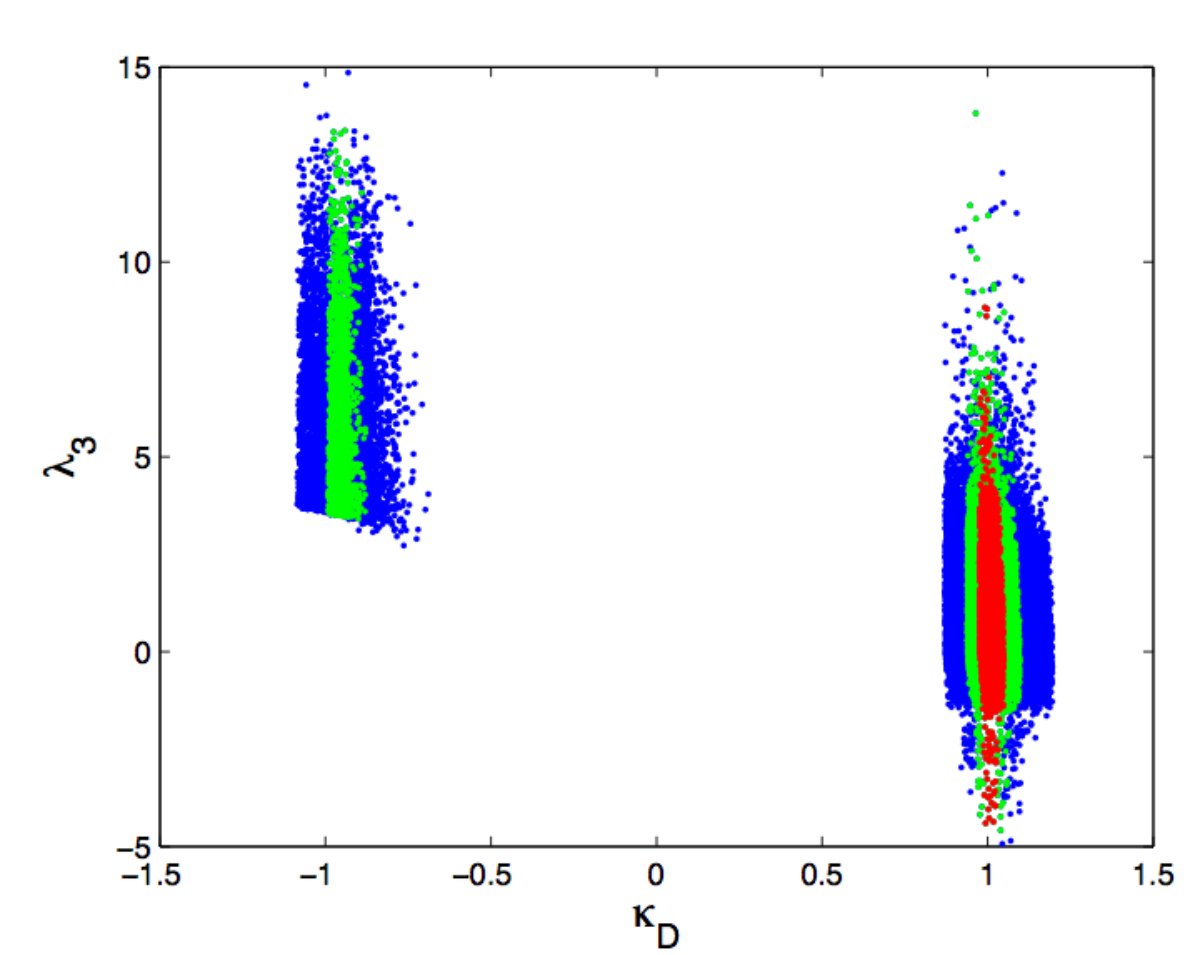
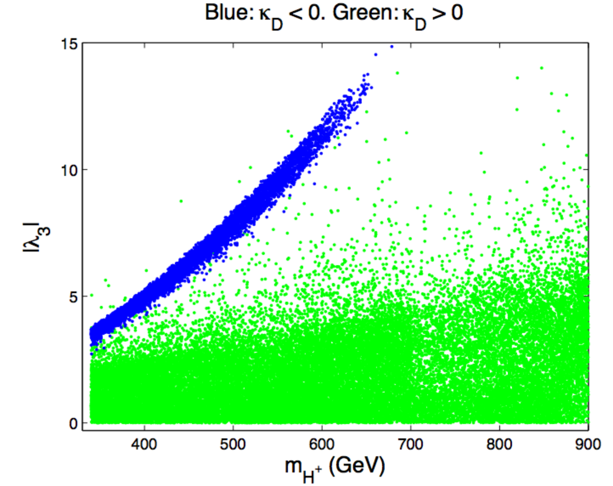
In Fig. 10, we show points in the vs. plane allowed when all the s are within 20%, 10% or 5% of unity. We see clearly that is limited to lie below about in the case while it can be arbitrarily large (we only scan up to ) for the standard scenario that allows for true decoupling. We have found that the maximum value is limited by the tree level unitarity limits of the , in particular . In Fig. 11, we display in the left panel as a function of for both the and scenarios; and in the right panel we show as a function of for the and scenarios requiring only that all s be within 20% of unity. Given that the tree level unitarity bounds on the are of order , we see that it is that encounters this upper limit at large in the case, whereas it is clear that in the case arbitrarily large is possible without violating tree level unitarity bounds, consistent with the decoupling limit. However, one should also note the significant number of points that hit the tree level unitarity bound for which nondecoupling is again possible.
The actual limits based on tree level unitarity bounds are imposed in terms of various amplitude combinations, of which it is
| (C.3) |
that is most constraining. In Fig. 12 we plot as a function of and of using the same format as in Fig. 11. Note that is hitting the tree level unitarity bound of for both the and scenarios. However, there is no limit on the associated value in the latter case, whereas there is the already quoted limit of in the former case.


We now show that for the type-II 2HDM with , where , and with , where (cf. Fig. 9), the loop functions are such that the charged-Higgs loop contributes with the same sign as the top-quark loop and thus will reduce the width, both canceling part of the -loop contribution of the opposite sign. As we have seen earlier, and will show numerically below, we find that this reduction is sufficient to prevent the channel from ever approaching the SM prediction and by an amount that will be seen at the LHC with high luminosity.
Let us now give more details. We will employ a simplified version of the the notation of CPsuperH [79]. One finds:
| (C.4) |
where
| (C.5) | |||||
with , , and the various ’s given by1313 13 Relative to Ref. [13], the defined here is one-half as large and has the opposite sign.
| (C.6) |
An explicit form for the function is defined in Eq. (40) of Ref. [79]. In the limit, , and . In eq. (C.5), and the other ’s are defined by the interaction Lagrangians,
| (C.7) |
where as defined in eq. (C.1).
In the case with we have , for which , and with the result
| (C.8) |
In the case we have , for which , , , and . For simplicity, consider and the limit of large . We then have,
| (C.9) |
The important thing to note here is that the loop contributes with the same sign as the top loop, i.e. it too will cancel against the negative -loop and decrease the width.
In more detail, we have the following. For both and , the relative contributions of the top-quark loop and the loop to are and . As regards the charged-Higgs loop, for and large one gets . As regards the -quark loop, for the case of we have . Of course, this changes sign for . We will neglect other quarks and leptons for simplicity since their contributions are quite small.
Then, in the SM case, neglecting the decoupled charged-Higgs loops, we find . If we consider the case without including the charged-Higgs loop one finds . The ratio of the absolute values is , a less than decrease in and certainly not measurable at the LHC. However, after including the charged-Higgs loop we obtain with the charged-Higgs loop evaluated at large , which translates to corresponding to a 12% decrease in . In fact, this level of decrease is very characteristic of the full scan as shown in Fig. 9 and is measurable at the LHC with and . As already noted, this same level of decrease also occurs for those scenarios for which the charged-Higgs loop does not decouple, i.e. roughly if (see Fig. 9).
Of course, in the computations presented in the main text, the full set of quarks and leptons is included, the charged-Higgs mass is varied as part of the scan (with the lower bound of ) and current LHC Higgs constraints are imposed as well as constraints from perturbativity, unitarity and precision electroweak measurements. As we have said above, all this leads to only small numerical changes relative to the decrease for quoted above; thus, the nondecoupling of the loop for leads to a decrease in that is at least as large as 5%.
References
- [1] G. Aad et al. [ATLAS Collaboration], Phys. Lett. B 716, 1 (2012) [arXiv:1207.7214 [hep-ex]].
- [2] S. Chatrchyan et al. [CMS Collaboration], Phys. Lett. B 716, 30 (2012) [arXiv:1207.7235 [hep-ex]].
- [3] G. Aad et al. [ATLAS Collaboration], Phys. Lett. B 726 (2013) 88 [arXiv:1307.1427 [hep-ex]].
- [4] S. Chatrchyan et al. [ CMS Collaboration], Phys. Rev. D 89, 092007 (2014) [arXiv:1312.5353 [hep-ex]].
- [5] M. Carena, C. Grojean, M. Kado and V. Sharma, in the 2013 partial update for the 2014 edition of J. Beringer et al. (Particle Data Group), Phys. Rev. D 86, 010001 (2012) [http://pdg.lbl.gov/2013/reviews/rpp2013-rev-higgs-boson.pdf].
- [6] J.R. Espinosa, C. Grojean, M. Mühlleitner and M. Trott, JHEP 1212 (2012) 045 [arXiv:1207.1717 [hep-ph]].
- [7] A. Falkowski, F. Riva and A. Urbano, JHEP 1311 (2013) 111 [arXiv:1303.1812 [hep-ph]].
- [8] G. Belanger, B. Dumont, U. Ellwanger, J.F. Gunion and S. Kraml, Phys. Rev. D 88, 075008 (2013) [arXiv:1306.2941 [hep-ph]].
- [9] A. Celis, V. Ilisie and A. Pich, JHEP 1312, 095 (2013) [arXiv:1310.7941 [hep-ph]].
- [10] P.M. Ferreira, R. Santos, M. Sher and J.P. Silva, Phys. Rev. D 85, 077703 (2012) [arXiv:1112.3277 [hep-ph]]; D. Carmi, A. Falkowski, E. Kuflik and T. Volansky, JHEP 1207 (2012) 136 [arXiv:1202.3144 [hep-ph]]; H.S. Cheon and S.K. Kang, JHEP 1309, 085 (2013) [arXiv:1207.1083 [hep-ph]]; W. Altmannshofer, S. Gori and G.D. Kribs, Phys. Rev. D 86, 115009 (2012) [arXiv:1210.2465 [hep-ph]]; Y. Bai, V. Barger, L.L. Everett and G. Shaughnessy, Phys. Rev. D 87, 115013 (2013) [arXiv:1210.4922 [hep-ph]]; C.-Y. Chen and S. Dawson, Phys. Rev. D 87, 055016 (2013) [arXiv:1301.0309 [hep-ph]]; A. Celis, V. Ilisie and A. Pich, JHEP 1307, 053 (2013) [arXiv:1302.4022 [hep-ph]]; C-W. Chiang and K. Yagyu, JHEP 1307, 160 (2013) [arXiv:1303.0168 [hep-ph]]; M. Krawczyk, D. Sokolowska and B. Swiezewska, J. Phys. Conf. Ser. 447, 012050 (2013) [arXiv:1303.7102 [hep-ph]]; B. Grinstein and P. Uttayarat, JHEP 1306, 094 (2013) [Erratum-ibid. 1309, 110 (2013)] [arXiv:1304.0028 [hep-ph]]; A. Barroso, P.M. Ferreira, R. Santos, M. Sher and J.P. Silva, arXiv:1304.5225 [hep-ph]; B. Coleppa, F. Kling and S. Su, JHEP 1401, 161 (2014) [arXiv:1305.0002 [hep-ph]]; P.M. Ferreira, R. Santos, M. Sher and J.P. Silva, arXiv:1305.4587 [hep-ph]; O. Eberhardt, U. Nierste and M. Wiebusch, JHEP 1307, 118 (2013) [arXiv:1305.1649 [hep-ph]]; S. Choi, S. Jung and P. Ko, JHEP 1310 (2013) 225 [arXiv:1307.3948 [hep-ph]]. V. Barger, L.L. Everett, H.E. Logan and G. Shaughnessy, Phys. Rev. D 88 (2013) 115003 [arXiv:1308.0052 [hep-ph]]; D. López-Val, T. Plehn and M. Rauch, JHEP 1310 (2013) 134 [arXiv:1308.1979 [hep-ph]]; S. Chang, S.K. Kang, J.-P. Lee, K.Y. Lee, S.C. Park and J. Song, arXiv:1310.3374 [hep-ph]; G. Cacciapaglia, A. Deandrea, G.D. La Rochelle and J.-B. Flament, arXiv:1311.5132 [hep-ph]; K. Cranmer, S. Kreiss, D. López-Val and T. Plehn, arXiv:1401.0080 [hep-ph];
- [11] K. Inoue, A. Kakuto, H. Komatsu and S. Takeshita, Prog. Theor. Phys. 67, 1889 (1982); R.A. Flores and M. Sher, Annals Phys. 148, 95 (1983); J.F. Gunion and H.E. Haber, Nucl. Phys. B 272, 1 (1986) [Erratum-ibid. B 402, 567 (1993)]; Nucl. Phys. B 278, 449 (1986) [Erratum-ibid. B 402, 569 (1993)].
- [12] T.D. Lee, Phys. Rev. D 8 (1973) 1226.
- [13] J.F. Gunion, H.E. Haber, G.L. Kane and S. Dawson, The Higgs Hunter’s Guide (Westview Press, Boulder, CO, 2000).
- [14] G.C. Branco, P.M. Ferreira, L. Lavoura, M.N. Rebelo, M. Sher and J.P. Silva, Phys. Rept. 516, 1 (2012) [arXiv:1106.0034 [hep-ph]].
- [15] S.L. Glashow and S. Weinberg, Phys. Rev. D 15, 1958 (1977); E.A. Paschos, Phys. Rev. D 15, 1966 (1977).
- [16] J.F. Gunion and H.E. Haber, Phys. Rev. D 67, 075019 (2003) [hep-ph/0207010].
- [17] P.M. Ferreira, R. Santos and A. Barroso, Phys. Lett. B 603 (2004) 219 [Erratum-ibid. B 629 (2005) 114] [hep-ph/0406231].
- [18] H.E. Haber, G.L. Kane and T. Sterling, Nucl. Phys. B 161, 493 (1979).
- [19] L.J. Hall and M.B. Wise, Nucl. Phys. B 187, 397 (1981).
- [20] J.F. Donoghue and L.F. Li, Phys. Rev. D 19, 945 (1979).
- [21] A. Arhrib, P.M. Ferreira and R. Santos, JHEP 1403, 053 (2014) [arXiv:1311.1520 [hep-ph]].
- [22] N.G. Deshpande and E. Ma, Phys. Rev. D 18 (1978) 2574.
- [23] S. Kanemura, T. Kubota and E. Takasugi, Phys. Lett. B 313 (1993) 155; A.G. Akeroyd, A. Arhrib and E.M. Naimi, Phys. Lett. B 490 (2000) 119.
- [24] M.E. Peskin and T. Takeuchi, Phys. Rev. D 46, 381 (1992).
- [25] C.D. Froggatt, R.G. Moorhouse and I.G. Knowles, Phys. Rev. D 45, 2471 (1992); W. Grimus, L. Lavoura, O.M. Ogreid and P. Osland, Nucl. Phys. B 801, 81 (2008) [arXiv:0802.4353 [hep-ph]]; H.E. Haber and D. O’Neil, Phys. Rev. D 83, 055017 (2011) [arXiv:1011.6188 [hep-ph]].
- [26] The ALEPH, CDF, D0, DELPHI, L3, OPAL, SLD Collaborations, the LEP Electroweak Working Group, the Tevatron Electroweak Working Group, and the SLD electroweak and heavy flavour Groups, arXiv:1012.2367 [hep-ex].
- [27] M. Baak, M. Goebel, J. Haller, A. Hoecker, D. Ludwig, K. Moenig, M. Schott and J. Stelzer, Eur. Phys. J. C 72, 2003 (2012) [arXiv:1107.0975 [hep-ph]].
- [28] M. Baak, M. Goebel, J. Haller, A. Hoecker, D. Kennedy, R. Kogler, K. Moenig, M. Schott and J. Stelzer, Eur. Phys. J. C 72, 2205 (2012) [arXiv:1209.2716 [hep-ph]].
- [29] A. Barroso, P.M. Ferreira, I.P. Ivanov and R. Santos, JHEP 1306 (2013) 045 [arXiv:1303.5098 [hep-ph]].
- [30] T. Hermann, M. Misiak and M. Steinhauser, JHEP 1211 (2012) 036 [arXiv:1208.2788 [hep-ph]]; M. Misiak, H.M. Asatrian, K. Bieri, M. Czakon, A. Czarnecki, T. Ewerth, A. Ferroglia and P. Gambino et al., Phys. Rev. Lett. 98, 022002 (2007) [hep-ph/0609232]; D. Asner et al. [Heavy Flavor Averaging Group Collaboration], arXiv:1010.1589 [hep-ex];
- [31] F. Mahmoudi and O. Stal, Phys. Rev. D 81, 035016 (2010) [arXiv:0907.1791 [hep-ph]]; S. Su and B. Thomas, Phys. Rev. D 79, 095014 (2009) [arXiv:0903.0667 [hep-ph]]; M. Aoki, S. Kanemura, K. Tsumura and K. Yagyu, Phys. Rev. D 80, 015017 (2009) [arXiv:0902.4665 [hep-ph]]; P. Posch, University of Vienna Ph.D. dissertation (2009).
- [32] A. Freitas and Y.-C. Huang, JHEP 1208, 050 (2012) [arXiv:1205.0299 [hep-ph]].
- [33] A. Denner, R.J. Guth, W. Hollik and J.H. Kuhn, Z. Phys. C 51, 695 (1991).
- [34] M. Boulware and D. Finnell, Phys. Rev. D 44, 2054 (1991).
- [35] A.K. Grant, Phys. Rev. D 51, 207 (1995) [hep-ph/9410267].
- [36] H.E. Haber and H.E. Logan, Phys. Rev. D 62, 015011 (2000) [hep-ph/9909335].
- [37] G. Abbiendi et al. [ALEPH and DELPHI and L3 and OPAL and LEP Collaborations], Eur. Phys. J. C 73 (2013) 2463 [arXiv:1301.6065 [hep-ex]].
- [38] ATLAS collaboration, ATLAS-CONF-2013-090; G. Aad et al. [ATLAS Collaboration], JHEP 1206 (2012) 039 [arXiv:1204.2760 [hep-ex]].
- [39] S. Chatrchyan et al. [CMS Collaboration], JHEP 1207 (2012) 143 [arXiv:1205.5736 [hep-ex]].
- [40] J.P. Lees et al. [BaBar Collaboration], Phys. Rev. Lett. 109, 101802 (2012) [arXiv:1205.5442 [hep-ex]].
- [41] J.F. Donoghue and L.F. Li, Phys. Rev. D 19, 945 (1979).
- [42] H. Georgi and D.V. Nanopoulos, Phys. Lett. 82B, 95 (1979).
- [43] F.J. Botella and J.P. Silva, Phys. Rev. D 51, 3870 (1995).
- [44] L. Lavoura and J.P. Silva, Phys. Rev. D 50, 4619 (1994);
- [45] L. Lavoura, Phys. Rev. D 50, 7089 (1994) [arXiv:hep-ph/9405307].
- [46] G.C. Branco, L. Lavoura and J.P. Silva, CP Violation (Oxford University Press, Oxford, England, 1999), Chapter 22.
- [47] S. Davidson and H.E. Haber, Phys. Rev. D 72, 035004 (2005) [Erratum-ibid. D 72, 099902 (2005)] [hep-ph/0504050].
- [48] H.E. Haber and Y. Nir, Nucl. Phys. B 335, 363 (1990).
- [49] M. Carena, H.E. Haber, H.E. Logan and S. Mrenna, Phys. Rev. D 65, 055005 (2002) [Erratum-ibid. D 65, 099902 (2002)] [hep-ph/0106116].
- [50] N. Craig, J. Galloway and S. Thomas, arXiv:1305.2424 [hep-ph].
- [51] D.M. Asner, T. Barklow, C. Calancha, K. Fujii, N. Graf, H.E. Haber, A. Ishikawa, S. Kanemura et al., arXiv:1310.0763 [hep-ph].
- [52] M. Carena, I. Low, N.R. Shah and C.E.M. Wagner, JHEP 1404, 015 (2014) [arXiv:1310.2248 [hep-ph]].
- [53] H.E. Haber, arXiv:1401.0152 [hep-ph]; and preprint in preparation.
- [54] H.E. Haber, M.J. Herrero, H.E. Logan, S. Penaranda, S. Rigolin and D. Temes, Phys. Rev. D 63, 055004 (2001) [hep-ph/0007006].
- [55] I.F. Ginzburg, M. Krawczyk and P. Osland, LC Note LC-TH-2001-026, [hep-ph/0101208]; Nucl. Instrum. Meth. A 472, 149 (2001) [hep-ph/0101229]; in Physics and Experiments with Future Linear Colliders, Batavia, Illinois, 2000, edited by A. Para and H. E. Fisk, AIP Conf. Proc. No. 578 (AIP, Melville, NY, 2001), pp. 304-311 [hep-ph/0101331].
- [56] I.F. Ginzburg and M. Krawczyk, Phys. Rev. D 72, 115013 (2005) [hep-ph/0408011].
- [57] A. Arhrib, R. Benbrik and C.-W. Chiang, Phys. Rev. D 77, 115013 (2008) [arXiv:0802.0319 [hep-ph]].
- [58] A. Arhrib, M. Capdequi Peyranere, W. Hollik and S. Penaranda, Phys. Lett. B 579, 361 (2004) [hep-ph/0307391].
- [59] G. Bhattacharyya, D. Das, P. B. Pal and M. N. Rebelo, JHEP 1310, 081 (2013) [arXiv:1308.4297 [hep-ph]].
- [60] A. David et al. [LHC Higgs Cross Section Working Group Collaboration], arXiv:1209.0040 [hep-ph].
- [61] S. Dawson, A. Gritsan, H. Logan, J. Qian, C. Tully, R. Van Kooten et al., arXiv:1310.8361 [hep-ex].
- [62] H. Ono and A. Miyamoto, Eur. Phys. J. C 73 (2013) 2343 [arXiv:1207.0300 [hep-ex]].
- [63] https://twiki.cern.ch/twiki/bin/view/LHCPhysics/CrossSectionsFigures#Higgs_production_cross_sections
- [64] R.V. Harlander and W.B. Kilgore, Phys. Rev. D 68, 013001 (2003) [hep-ph/0304035].
- [65] M. Spira, arXiv:hep-ph/9510347.
- [66] B. Dumont, J.F. Gunion, Y. Jiang and S. Kraml, arXiv:1405.3584 [hep-ph].
- [67] A. Djouadi, J. Kalinowski and M. Spira, Comput. Phys. Commun. 108 (1998) 56 [hep-ph/9704448].
- [68] R. Harlander, M. Mühlleitner, J. Rathsman, M. Spira and O. Stål, arXiv:1312.5571 [hep-ph].
- [69] D. Eriksson, J. Rathsman and O. Stål, Comput. Phys. Commun. 181 (2010) 189 [arXiv:0902.0851 [hep-ph]].
- [70] H.E. Haber and D. O’Neil, Phys. Rev. D 74, 015018 (2006) [Erratum-ibid. D 74, 059905 (2006)] [hep-ph/0602242].
- [71] M. Carena and H.E. Haber, Prog. Part. Nucl. Phys. 50, 63 (2003) [hep-ph/0208209].
- [72] A. Djouadi, Phys. Rept. 459, 1 (2008) [hep-ph/0503173].
- [73] H.E. Haber and R. Hempfling, Phys. Rev. Lett. 66, 1815 (1991); J.R. Ellis, G. Ridolfi and F. Zwirner, Phys. Lett. B 257, 83 (1991); Y. Okada, M. Yamaguchi and T. Yanagida, Prog. Theor. Phys. 85, 1 (1991).
- [74] H.E. Haber and R. Hempfling, Phys. Rev. D 48, 4280 (1993) [hep-ph/9307201].
- [75] H.E. Haber and J.D. Mason, Phys. Rev. D 77, 115011 (2008) [arXiv:0711.2890 [hep-ph]].
- [76] M. Carena, D. Garcia, U. Nierste and C.E.M. Wagner, Nucl. Phys. B 577, 88 (2000) [hep-ph/9912516].
- [77] R. Hempfling, Phys. Rev. D 49, 6168 (1994); L.J. Hall, R. Rattazzi and U. Sarid, Phys. Rev. D 50, 7048 (1994) [hep-ph/9306309]; M. Carena, M. Olechowski, S. Pokorski and C.E.M. Wagner, Nucl. Phys. B 426, 269 (1994) [hep-ph/9402253]; D.M. Pierce, J.A. Bagger, K.T. Matchev and R.-J. Zhang, Nucl. Phys. B 491, 3 (1997) [hep-ph/9606211].
- [78] M. Carena, S. Heinemeyer, O. Stål, C.E.M. Wagner and G. Weiglein, Eur. Phys. J. C 73, 2552 (2013) [arXiv:1302.7033 [hep-ph]].
- [79] J.S. Lee, A. Pilaftsis, M. Carena, S.Y. Choi, M. Drees, J.R. Ellis and C.E.M. Wagner, Comput. Phys. Commun. 156, 283 (2004) [hep-ph/0307377].