Abstract: Consider a network whose nodes have some initial values, and it is desired to design an algorithm that builds on neighbor to neighbor interactions with the ultimate goal of convergence to the average of all initial node values or to some value close to that average. Such an algorithm is called generically “distributed averaging”, and our goal in this paper is to study the performance of a subclass of deterministic distributed averaging algorithms where the information exchange between neighboring nodes (agents) is subject to uniform quantization. With such quantization, convergence to the precise average cannot be achieved in general, but the convergence would be to some value close to it, called quantized consensus. Using Lyapunov stability analysis, we characterize the convergence properties of the resulting nonlinear quantized system. We show that in finite time and depending on initial conditions, the algorithm will either cause all agents to reach a quantized consensus where the consensus value is the largest quantized value not greater than the average of their initial values, or will lead all variables to cycle in a small neighborhood around the average. In the latter case, we identify tight bounds for the size of the neighborhood and we further show that the error can be made arbitrarily small by adjusting the algorithm’s parameters in a distributed manner.

Key-words: distributed averaging, quantization, finite state automata, cycle, quantized consensus

Conception et Analyse d’Algorithmes Distribués de Moyennage avec Valeurs Échangées Discrétisées

Résumé : Nous allons nous intéresser à un réseau dont les nœuds, ou agents, ont des valeurs initiales. Nous souhaitons concevoir un algorithme ayant pour objectif la convergence vers une valeur qui est la plus proche possible de la moyenne de toutes les valeurs initiales des nœuds. Cette algorithme est basée sur les interaction entre les nœuds, où un nœud interagit avec un autre nœud si ils sont voisins dans le graphe. Un tel algorithme est communément appelé “moyenne distribuée”. L’objectif de cet article est d’étudier les performances d’une sous-classe d’algorithmes déterministes de calcul de la moyenne distribuée, où l’échange d’informations entre les nœuds voisins est soumis à la quantification uniforme. Avec une telle quantification, la moyenne précise ne peut être atteinte (sauf dans des cas exceptionnels), mais une valeur proche d’elle peut être atteinte. Cette valeur est appelée consensus quantifié. Nous montrons dans ce papier que, dans un temps fini, soit tous les agents parviennent à un consensus quantifié où la valeur de consensus est le plus grand entier qui n’est pas supérieur à la moyenne de leurs valeurs initiales; ou soit tous les agents cyclent dans un petit voisinage autour de la moyenne, en fonction des conditions initiales. Dans ce dernier cas, il est démontré que le voisinage peut être rendue arbitrairement faible en ajustant les paramètres de l’algorithme de manière distribuèe.

Mots-clés : distributed averaging, quantization, finite state automata, cycle, quantized consensus

1 Introduction

There has been considerable interest recently in developing algorithms for distributing information among members of interactive agents via local interactions (e.g., a group of sensors [2] or mobile autonomous agents [30]), especially for the scenarios where agents or sensors are constrained by limited sensing, computation, and communication capabilities. Notable among these are those algorithms intended to cause such a group to reach a consensus in a distributed manner [38, 23, 7]. Consensus processes play an important role in many other problems such as Google’s PageRank [22], clock synchronization [34], and formation control [19].

One particular type of consensus process, distributed averaging, has received much attention lately [39, 16, 17, 29]. In its simplest form, distributed averaging deals with a network of $n>1$ agents and the constraint that each agent $i$ is able to communicate only with certain other agents called agent $i$ ’s neighbors. Neighbor relations are conveniently characterized by a simple, connected graph in which vertices correspond to agents and edges indicate neighbor relations. Each agent $i$ initially has or acquires a real number $z_{i}$ which might be a measurement value.The distributed averaging problem is to devise an algorithm which will enable each agent to compute the average $z_{ave}=\frac{1}{n}\sum_{i=1}^{n}z_{i}$ using only information acquired from its neighbors.

Most existing algorithms for precise distributed averaging require that agents are able to send and receive real values with infinite precision. However, a realistic network can only allow messages with limited length to be transmitted between agents due to constraints on the capacity of communication links. With such a constraint, when a real value is sent from an agent to its neighbors, this value will be truncated and only a quantized version will be received by the neighbors. With such quantization, the precise average cannot be achieved (except in particular cases), but some value close to it can be achieved, called quantized consensus. A number of papers have studied this quantized consensus problem and various probabilistic strategies have been proposed to cause all the agents in a network to reach a quantized consensus with probability one (or at least with high probability) [35, 3, 4, 5, 6, 26, 24, 25, 18]. Notwithstanding this, the problem of how to design and analyze deterministic algorithms for quantized consensus remains open [20, 12].

In this paper, we thoroughly analyze the performance of a deterministic distributed averaging algorithm where the information exchange between neighboring agents is subject to uniform quantization. It is shown that in finite time, the algorithm will either cause all $n$ agents to reach a quantized consensus where the consensus value is the largest integer not greater than the average of their initial values, or will lead all $n$ agents’ variables to cycle in a small neighborhood around the average, depending on initial conditions. In the latter case, it is further shown that the neighborhood can be arbitrarily small by adjusting the algorithm’s parameters in a distributed manner.

The rest of the paper is organized as follows: in Section 2 we review the existing literature related to our work. In Section 3 we introduce some preliminaries of distributed averaging. A network model for quantized communications is given in Section 4 . In Section 5, we formulate the problem considered in this paper and present the equation model of the quantized system. The design and analysis of the system, including the main results of the paper, are given in Section 6. A further discussion is given in Section 7. Section 8 provides some simulations supporting our analytic results and Section 9 concludes the paper.

2 Literature Review

Most of the related works for distributed averaging with quantized communication propose either a deterministic algorithm (as our approach in this paper) or a probabilistic one.

There are only a few publications which study deterministic algorithms for quantized consensus. In [27] the distributed averaging problem with quantized communication is formulated as a feedback control design problem for coding/decoding schemes; the paper characterizes the amount of information needed to be sent for the agents to reach a consensus and shows that with an appropriate scaling function and some carefully chosen control gain, the proposed protocol can solve the distributed averaging problem, but some spectral properties of the Laplacian matrix of the underlying fixed undirected graph have to be known in advance. More sophisticated coding/decoding schemes were proposed in [28] for time-varying undirected graphs and in [42] for time-varying directed graphs, all requiring carefully chosen parameters. Recently a novel dynamic quantizer has been proposed in [37] based on dynamic quantization intervals for coding of the exchanged messages in wireless sensor networks leading to asymptotic convergence to consensus. In [15] a biologically inspired algorithm was proposed which will cause all $n$ agents to reach some consensus with arbitrary precision, but at the cost of not preserving the desired average. Control performance of logarithmic quantizers was studied in [13] and quantization effects were considered in [32]. A deterministic algorithm of the same form as in this paper has been only partially analyzed in [20] where the authors have approximated the system by a probabilistic model and left the design of the weights as an open problem.

Over the past decade quite a few probabilistic quantized consensus algorithms have been proposed. The probabilistic quantizer in [4] ensures almost surely consensus at a common but random quantization level for fixed (strongly connected) directed graphs; although the expectation of the consensus value equals the desired average, the deviation of the consensus value from the desired average is not tightly bounded. An alternative algorithm which gets around this limitation was proposed in [24]; the algorithm adds dither to the agents’ variables before quantization and the mean square error can be made arbitrarily small by tuning the parameters. The probabilistic algorithm in [5, 6], called “interval consensus gossip”, causes all $n$ agents to reach a consensus in finite time almost surely on the interval in which the average lies, for time-varying (jointly connected) undirected graphs. A stochastic quantized gossip algorithm was shown to work properly in [26]. The effects of quantized communication on the standard randomized gossip algorithm [9] were analyzed in [14]. An alternative approach to analyze the quantization effect was introduced in [35, 3] which model the effect as noise following certain probability.

Another thread of research has studied quantized consensus with the additional constraint that the value at each node is an integer. The probabilistic algorithm in [25] causes all $n$ agents to reach quantized consensus almost surely for a fixed (connected) undirected graph; convergence time of the algorithm was studied in [18], with strong bounds on its expected value. In [11] a probabilistic algorithm was proposed to solve the quantized consensus problem for fixed (strongly connected) directed graphs using the idea of “surplus”.

We should note that, in addition, our work in this paper is also related to the literature on the problem of load balancing [1, 36, 21].

3 Distributed Averaging

Consider a group of $n>1$ agents labeled $1$ to $n$ . Each agent $i$ has control over a real-valued scalar quantity $x_{i}$ called an agreement variable which the agent is able to update its value from time to time. Agents may only communicate with their “neighbors”. Agent $j$ is a neighbor of agent $i$ if $(i,j)\in\mathcal{E}$ is an edge in a given simple, undirected $n$ -vertex graph $\mathbb{G}=(\mathcal{V},\mathcal{E})$ where $\mathcal{V}=\{1,2,\ldots,n\}$ is the vertex set and $\mathcal{E}$ is the edge set. We assume that the graph $\mathbb{G}$ is connected and does not change over time. Initially each agent $i$ has a real number $x_{i}(0)$ . Let

x_{ave}(k)=\frac{1}{n}\sum_{i\in\mathcal{V}}x_{i}(k),

be the average of values of all agreement variables in the network, we will refer to $x_{ave}(0)$ simply as $x_{ave}$ . The purpose of the distributed averaging problem is to devise an algorithm which enables all $n$ agents to asymptotically determine in a decentralized manner, the average of the initial values of their scalar variables, i.e.,

\lim_{k\rightarrow\infty}x_{i}(k)=x_{ave}.

A well studied approach to the problem is for each agent to use a linear iterative update rule of the form

x_{i}(k+1)=w_{ii}x_{i}(k)+\sum_{j\in\mathcal{N}_{i}}w_{ij}x_{j}(k),\ \ \forall i\in\mathcal{V},

(1)

where $k$ is a discrete time index, $\mathcal{N}_{i}$ is the set of neighbors of agent $i$ and the $w_{ij}$ are real-valued weights to be designed. In [8] several methods are proposed for choosing the weights $w_{ij}$ with the goal of obtaining algorithms with improved convergence rates. One particular choice, which defines what has come to be known as the Metropolis algorithm, requires only local information to define the $w_{ij}$ [41, 40]. The corresponding Metropolis weights are chosen as follows:

	$\displaystyle w_{ij}$	$\displaystyle=$	$\displaystyle\frac{1}{\text{max}\{d_{i},d_{j}\}+1},\ \ \forall(i,j)\in\mathcal{E},$
	$\displaystyle w_{ii}$	$\displaystyle=$	$\displaystyle 1-\sum_{j\in\mathcal{N}_{i}}w_{ij},\ \ \forall i\in\mathcal{V},$

where $d_{i}$ is the degree of agent $i$ .

Eq. (1) can be written in a matrix form as

\mathbf{x}(k+1)=W\mathbf{x}(k),

where $\mathbf{x}(k)$ is the state vector of agreement values whose $i$ th element equals $x_{i}(k)$ , and $W$ is the weight matrix whose $ij$ th entry equals $w_{ij}$ . It should be clear that $w_{ij}>0$ if $(i,j)\in\mathcal{E}$ and $w_{ij}=0$ otherwise. A necessary and sufficient condition for the convergence of Eq. (1) to the desired average for any initial values is that $W$ is a doubly stochastic matrix and all eigenvalues of $W$ , with the exception of a single eigenvalue of value $1$ , have magnitude strictly less than unity [39]. It is easy to verify that the Metropolis weights satisfy this condition. Thus the Metropolis weights guarantee the desired convergence, i.e.,

\lim_{k\rightarrow\infty}\mathbf{x}(k)=x_{ave}\mathbf{1},

where $\mathbf{1}$ is the vector in $\mathbb{R}^{n}$ whose entries all equal one. It is worth noting that since $W$ is doubly stochastic, the summation of all $n$ values of agreement variables is kept constant, so is the average of the variables, namely

\mathbf{1}^{T}\mathbf{x}(k)=\mathbf{1}^{T}\mathbf{x}(0)=nx_{ave},\ \forall k.

4 Quantized Communication

In a network where links have constraints on the capacity and have limited bandwidth (e.g., digital communication networks), messages cannot have infinite length. However, the distributed averaging algorithm requires sending real (infinite precision) values through these communication links. Therefore, with digital transmission, the messages transmitted between neighboring agents will have to be truncated. If the communication bandwidth was limited, the more the truncation of agents’ values, the higher would be the deviation of agent’s value from the desired average consensus $x_{ave}$ .

To model the effect of quantized communication, we assume that the links perform a quantization effect on the values transmitted between agents. The network model is given by Fig. 1.

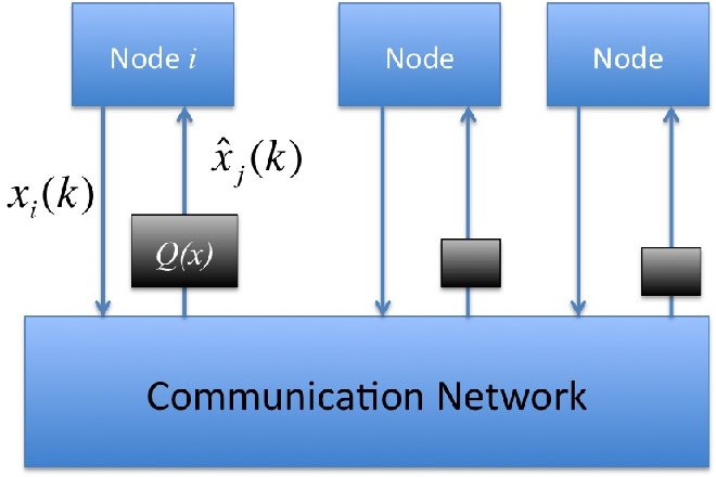
Refer to caption — Figure 1: The network model for the quantized system.

As we can see from the model, each agent $i$ can have infinite bandwidth to store its latest value $x_{i}(k)$ and perform computations. However, when agent $i$ sends its value at time $k$ through the communication network, its neighbors will receive a value $\hat{x}_{i}(k)$ which is the quantized value of $x_{i}(k)$ . A quantizer is a function $\mathcal{Q}:\mathbb{R}\rightarrow\mathbb{Z}$ that maps a real value to an integer. Quantizers can be of different forms. We present here some widely used quantizers in the literature [31, 14, 32]:

1.

Truncation quantizer $\mathcal{Q}_{t}$ which truncates the decimal part of a real number and keeps the integer part:

$\displaystyle\mathcal{Q}_{t}(x)$ $\displaystyle=\lfloor x\rfloor.$ (2)
2.

Ceiling quantizer $\mathcal{Q}_{c}$ which rounds the value to the nearest upper integer:

$\displaystyle\mathcal{Q}_{c}(x)$ $\displaystyle=\lceil x\rceil.$ (3)

Rounding quantizer $\mathcal{Q}_{r}$ which rounds a real number to its nearest integer:

\displaystyle\mathcal{Q}_{r}(x)

\displaystyle=\begin{cases}\lfloor x\rfloor&\text{ if }x-\lfloor x\rfloor<1/2\\ \lceil x\rceil&\text{ if }x-\lfloor x\rfloor\geq 1/2.\end{cases}

(4)

Probabilistic quantizer $\mathcal{Q}_{p}$ defined as follows:

\displaystyle\mathcal{Q}_{p}(x)=\begin{cases}\lfloor x\rfloor&\text{ with probability }\lceil x\rceil-x\\ \lceil x\rceil&\text{ with probability }x-\lfloor x\rfloor.\end{cases}

(5)

In this report we study the effect of the deterministic quantizers ( $\mathcal{Q}_{t}(x)$ , $\mathcal{Q}_{c}(x)$ , and $\mathcal{Q}_{r}(x)$ ) on the performance of the distributed averaging algorithms by showing the distance that the agents’ stored values can deviate from the initial average $x_{ave}$ . The quantizers listed before map $\mathbb{R}$ into $\mathbb{Z}$ and have quantization jumps of size 1. Quantizers having a generic real positive quantization step $\epsilon$ can be simply recovered by a suitable scaling: $\mathcal{Q}^{(\epsilon)}(x)=\epsilon\mathcal{Q}(x/\epsilon)$ [14]. Thus the results in this report cover these generic quantizers as well.

5 Problem Formulation

Suppose that all $n$ agents adhere to the same update rule of Eq. (1). Then with a quantizer $\mathcal{Q}(x)$ , the network equation would be

x_{i}(k+1)=w_{ii}x_{i}(k)+\sum_{j\in\mathcal{N}_{i}}w_{ij}\mathcal{Q}(x_{j}(k)),\ \ \forall i\in\mathcal{V}.

(6)

Simple examples show that this algorithm can cause the system to shift away from the initial average $x_{ave}$ .

Since agents know exactly the effect of the quantizer, for the agents not to lose any information caused by quantization, at each iteration $k$ each agent $i$ can send out the quantized value $\mathcal{Q}(x_{i}(k))$ (instead of sending $x_{i}(k)$ ) and store in a local scalar $c_{i}(k)$ the difference between the real value $x_{i}(k)$ and its quantized version, i.e.,

\displaystyle c_{i}(k)

\displaystyle=x_{i}(k)-\mathcal{Q}(x_{i}(k)).

Then, the next iteration update of agent $i$ can be modified to be

x_{i}(k+1)=w_{ii}\mathcal{Q}(x_{i}(k))+\sum_{j\in\mathcal{N}_{i}}w_{ij}\mathcal{Q}(x_{j}(k))+c_{i}(k),\ \ \forall i\in\mathcal{V}.

(7)

A major difference between this equation and (6) is that here no information is lost; i.e., the total average is being conserved in the network, as we will show shortly after. The state equation of the system becomes,

\mathbf{x}(k+1)=W\mathcal{Q}\left(\mathbf{x}(k)\right)+\mathbf{x}(k)-\mathcal{Q}\left(\mathbf{x}(k)\right),

(8)

where, with a little abuse of notation, $\mathcal{Q}\left(\mathbf{x}\right)=\left(\mathcal{Q}(x_{1}),\mathcal{Q}(x_{2}),\dots,\mathcal{Q}(x_{n})\right)^{T}$ is the vector quantization operation. For any $W$ where each column sums to $1$ ( $\mathbf{1}^{T}W=\mathbf{1}^{T}$ where $\mathbf{1}$ is the vector of all ones), the total sum of all $n$ agreement variables does not change over time if agents followed the protocol of Eq. (8):

$\displaystyle\mathbf{1}^{T}\mathbf{x}(k+1)$	$\displaystyle=\mathbf{1}^{T}(W\mathcal{Q}\left(\mathbf{x}(k)\right)+\mathbf{1}^{T}\mathbf{x}(k)-\mathbf{1}^{T}\lfloor\mathbf{x}(k)\rfloor$
	$\displaystyle=\mathbf{1}^{T}\mathcal{Q}\left(\mathbf{x}(k)\right)+\mathbf{1}^{T}\mathbf{x}(k)-\mathbf{1}^{T}\mathcal{Q}\left(\mathbf{x}(k)\right)$
	$\displaystyle=\mathbf{1}^{T}\mathbf{x}(k)$
	$\displaystyle=\mathbf{1}^{T}\mathbf{x}(0)$
	$\displaystyle=nx_{ave},$	(9)

Thus the average is also conserved ( $x_{ave}(k)=x_{ave},\;\;\forall k$ ). Equation (8) would be our model of distributed averaging with deterministic quantized communication where the quantizer can take the form of the truncation $\mathcal{Q}_{t}$ , the ceiling $\mathcal{Q}_{c}$ , or the rounding one $\mathcal{Q}_{r}$ . It is worth noting that the three quantizers can be related by the following equations:

	$\displaystyle\mathcal{Q}_{r}(x)$	$\displaystyle=\mathcal{Q}_{t}(x+1/2),$		(10)
	$\displaystyle\mathcal{Q}_{c}(x)$	$\displaystyle=-\mathcal{Q}_{t}(-x).$		(11)

Given a model with the ceiling quantizer $\mathcal{Q}_{c}$ in (8), by taking $\mathbf{y}(k)=-\mathbf{x}(k)$ , the system evolves as:

	$\displaystyle\mathbf{y}(k+1)$	$\displaystyle=\mathbf{y}(k)+W\mathcal{Q}_{t}(\mathbf{y}(k))-\mathcal{Q}_{t}(\mathbf{y}(k))$
	$\displaystyle\mathbf{y}(0)$	$\displaystyle=-\mathbf{x}(0).$

Therefore, by analyzing the above system which has a truncation quantizer $\mathcal{Q}_{t}$ , we can deduce the performance of $\mathbf{x}(k)$ that satisfies equation (8) with a ceiling quantizer $\mathcal{Q}_{c}$ because they are related by a simple equation ( $\mathbf{y}(k)=-\mathbf{x}(k)$ ).

Similarly, given a model with the rounding quantizer $\mathcal{Q}_{r}$ in (8), by taking $\mathbf{y}(k)=\mathbf{x}(k)+\frac{1}{2}\mathbf{1}$ , the system evolves as:

	$\displaystyle\mathbf{y}(k+1)$	$\displaystyle=\mathbf{y}(k)+W\mathcal{Q}_{t}(\mathbf{y}(k))-\mathcal{Q}_{t}(\mathbf{y}(k))$
	$\displaystyle\mathbf{y}(0)$	$\displaystyle=\mathbf{x}(0)+\frac{1}{2}\mathbf{1}.$

Therefore, by analyzing the above system which has a truncation quantizer $\mathcal{Q}_{t}$ , we can deduce the performance of $\mathbf{x}(k)$ that satisfies equation (8) with a rounding quantizer $\mathcal{Q}_{r}$ because they are related by a simple translation equation ( $\mathbf{y}(k)=\mathbf{x}(k)+\frac{1}{2}\mathbf{1}$ ). Therefore the effects of all these three quantizers are essentially the same.

With this nontrivial observation in mind, we focus on the analysis of the truncation quantizer only in the rest of this report. The results can then be easily extended to the case of the other two quantizers.

In the sequel we will fully characterize the behavior of system (8) and its convergence properties. But first, we have the following definition:

Definition 1.

A network of $n$ agents reaches quantized consensus if there is an iteration $k_{0}$ such that

\mathcal{Q}(x_{i}(k))=\mathcal{Q}(x_{j}(k)),\;\;\forall i,j\in\mathcal{V},\ \forall k\geq k_{0}.

6 Design and Analysis of the System

In this section, we carry out the analysis of the proposed quantized system equation. By considering the truncation quantizer $\mathcal{Q}_{t}$ in (8), the system equation becomes:

\mathbf{x}(k+1)=W\lfloor\mathbf{x}(k)\rfloor+\mathbf{x}(k)-\lfloor\mathbf{x}(k)\rfloor.

(12)

This can be written in a distributed way for every $i\in\mathcal{V}$ as follows:

	$\displaystyle x_{i}(k+1)$	$\displaystyle=x_{i}(k)+\sum_{j\in\mathcal{N}_{i}}w_{ji}\left(\lfloor x_{j}(k)\rfloor-\lfloor x_{i}(k)\rfloor\right),$		(13)
		$\displaystyle=x_{i}(k)+\sum_{j\in\mathcal{N}_{i}}w_{ji}L_{ji}(k),$		(14)

where

L_{ji}(k)\triangleq\lfloor x_{j}(k)\rfloor-\lfloor x_{i}(k)\rfloor=-L_{ij}(k).

The non-linearity of the system due to quantization complicates the analysis, and traditional stability analysis of linear systems (such as ergodicity, products of stochastic matrices, etc.) cannot be applied here as the system might not even converge. As demonstrated in the following subsection.

6.1 Cyclic Example

The purpose of the following example is to show that for a “bad” weight matrix design, the quantized system can cycle very far from the average. Consider the two-nodes example of Fig. 2,

suppose that $x_{a}(0)=\xi$ , $x_{b}(0)=K+\xi$ where $K\in\mathbb{N}$ and $\xi\in(0,1)$ . With these initial values, $\lfloor x_{a}(0)\rfloor=0$ , $\lfloor x_{b}(0)\rfloor=K$ , and $x_{ave}=\frac{K}{2}+\xi$ . The weight matrix for this two-nodes system is assumed to be a doubly stochastic matrix and is given as follows:

W=\left(\begin{array}[]{cc}w&1-w\\ 1-w&w\end{array}\right),

where $w\in(0,1)$ . With this weight matrix, (9) is satisfied and the average is conserved. In [20], the authors defined the following metric to measure the performance of the system:

d_{\infty}(W,\mathbf{x}(0))=\limsup_{k\rightarrow\infty}\frac{1}{\sqrt{n}}||\Delta(k)||,

(15)

where $\Delta(k)$ is a vector having the elements $\Delta_{i}(k)=x_{i}(k)-x_{ave}$ . So the worst cycle (according to this metric), given a doubly stochastic weight matrix, would happen if the nodes toggled their values with every iteration. Let us derive conditions on $W$ for which this could happen. With the quantization, the corresponding system equations are as follows:

	$\displaystyle x_{a}(k+1)$	$\displaystyle=x_{a}(k)+(1-w)\times\left(\lfloor x_{b}(k)\rfloor-\lfloor x_{a}(k)\rfloor\right)$		(16)
	$\displaystyle x_{b}(k+1)$	$\displaystyle=x_{b}(k)+(1-w)\times\left(\lfloor x_{a}(k)\rfloor-\lfloor x_{b}(k)\rfloor\right).$		(17)

From the given initial conditions, after one iteration the updated values are $x_{a}(1)=\xi+(1-w)K$ and $x_{b}(1)=K+\xi-(1-w)K$ . Therefore, the quantized value of the nodes’ variables will toggle between $0$ and $K$ if $x_{a}(1)\in[K,K+1)$ and $x_{b}(1)\in[0,1)$ . By substituting the values of $x_{a}(1)$ and $x_{b}(1)$ we get the following conditions for such a cycle,

\begin{cases}wK>\max\{-\xi,\xi-1\}\\ wK<\min\{\xi,1-\xi\}.\end{cases}

(18)

The first condition is always satisfied because $wK>0$ . Then, a bad design of $W$ is to have $w<\frac{1}{K}\times\min\{\xi,1-\xi\}$ because in this case the nodes can cycle¹¹ 1 In case initial values were not known, since $\min\{\xi,1-\xi\}\leq 1/2$ , then, a bad design of $W$ is to have $w<\frac{1}{2K}$ because in this case there might be some initial values that cause large cycles. with

x_{a}(k)=\begin{cases}\xi&\text{ if $k$ is even}\\ K+\xi-wK&\text{ if $k$ is odd}\end{cases}\ \ \text{and }\ \ x_{b}(k)=\begin{cases}K+\xi&\text{ if $k$ is even}\\ wK+\xi&\text{ if $k$ is odd}.\end{cases}

(19)

Thus $\Delta_{a}(k)=\Delta_{b}(k)=K/2$ if $k$ is even, and so $d_{\infty}(W,\mathbf{x}(0))=K/2$ . The above two-node network result can be extended to regular bipartite graphs where the first set of nodes takes the value $x_{a}(0)$ and the other set takes the value $x_{b}(0)$ and all self-weights are equal to $w$ .²² 2 In case of hypercube graphs, [20] shows that if the weights in the network have a constant value $1/(d+1)$ where $d=\log n$ is the degree of a node in the hypercube graph, then an upper bound on $d_{\infty}(W)=\sup_{\mathbf{x}(0)}d_{\infty}(W,\mathbf{x}(0))$ is the following $d_{\infty}(W)\leq\frac{\log n}{2}$ . Since a hypercube is a regular bipartite graph, then using our results leads to the following lower bound, $d_{\infty}(W)\geq\frac{\log n}{4}$ (by taking $\xi=0.5$ and $K=(\log n)/2$ to satisfy (18)). This would also lead to the following inequality on $d_{\infty}(W,\mathbf{x}(0))$ with the given initial conditions and weight matrix:

d_{\infty}(W,\mathbf{x}(0))\geq K/2.

This shows that a bad design of $W$ on general graphs can make the cycle arbitrarily large.

6.2 Weight Assumption

The system behavior depends of course on the design of the weight matrix. In distributed averaging, it is important to consider weights that can be chosen locally, avoid bad design, and guarantee desired convergence properties. We impose the following assumption on $W$ which can be satisfied in a distributed manner.

Assumption 1.

The weight matrix in our design has the following properties:

•

$W$ is a symmetric doubly stochastic matrix:

$\displaystyle w_{ij}=w_{ji}\geq 0\ \ \forall i,j\in\mathcal{V}$

$\displaystyle\sum_{i}w_{ij}=\sum_{j}w_{ij}=1,$
•

Dominant diagonal entries of $W$ :

$w_{ii}>1/2\text{ for all }i\in\mathcal{V},$
•

Network communication constraint: if $(i,j)\notin\mathcal{E}$ , then $w_{ij}=0$ ,
•

For any link $(i,j)\in\mathcal{E}$ we have $w_{ij}\in\mathbb{Q}^{+}$ , where $\mathbb{Q}^{+}$ is the set of rational numbers in the interval $(0,1)$ .

These are also sufficient conditions for the linear system (1) to converge. The choice of weights being rational numbers is not restrictive because any practical implementation would satisfy this property intrinsically (we use it here to prove convergence results). The dominant diagonal entries assumption is very important to prevent the system from having large cycles (as in the cyclic example in Section 6.1).

We now state the main result of this report which will be proved in the following subsections.

Main Convergence Result 1.

Consider the quantized system (12). Suppose that Assumption 1 holds. Then for any initial value $\mathbf{x}(0)$ , there is a finite time iteration where either

1.

the system reaches quantized consensus, or
2.

the nodes’ values cycle in a small neighborhood around the average, where the neighborhood can be made arbitrarily small by a decentralized design of the weights (having trade-off with the speed of convergence).

To highlight the importance of these results, notice that the Main Convergence Result 1 implies there is an iteration $k_{0}$ such that $x_{i}(k)-x_{j}(k)<1$ for all $i,j\in\mathcal{V}$ for $k\geq k_{0}$ . This gives a constant upper bound on the metric $d_{\infty}(W,\mathbf{x}(0))$ independent of initial values, i.e., due to Assumption 1, $d_{\infty}(W,\mathbf{x}(0))\leq 0.5$ on any general graph and for any initial conditions.

6.3 Cyclic States

We study in this subsection the convergence properties of the system equation (12) under Assumption 1. Let us first show that due to quantized communication, the states of the agents lie in a discrete set. Since $w_{ij}\in\mathbb{Q}^{+}$ for any link $(i,j)$ , we can write

w_{ij}=\frac{a_{ij}}{b_{ij}},

where $a_{ij}$ and $b_{ij}$ are co-prime positive integers. Suppose that $B_{i}$ is the Least Common Multiple (LCM) of the integers $\{b_{ij};(i,j)\in\mathcal{E},j\in\mathcal{N}_{i}\}$ . Let $c_{i}(k)=x_{i}(k)-\lfloor x_{i}(k)\rfloor$ ; then we have $c_{i}(k)\in[0,1)$ . Let us see how $c_{i}(k)$ evolves:

$\displaystyle c_{i}(k)$	$\displaystyle=x_{i}(k)-\lfloor x_{i}(k)\rfloor$
	$\displaystyle=x_{i}(k-1)+\sum_{j\in\mathcal{N}_{i}}w_{ij}\times\left(\lfloor x_{j}(k-1)\rfloor-\lfloor x_{i}(k-1)\rfloor\right)$
	$\displaystyle\hskip 14.22636pt-\lfloor x_{i}(k)\rfloor$
	$\displaystyle=\lfloor x_{i}(k-1)\rfloor+c_{i}(k-1)$
	$\displaystyle\hskip 14.22636pt+\sum_{j\in\mathcal{N}_{i}}\frac{a_{ij}}{b_{ij}}\times\left(\lfloor x_{j}(k-1)\rfloor-\lfloor x_{i}(k-1)\rfloor\right)-\lfloor x_{i}(k)\rfloor$
	$\displaystyle=c_{i}(k-1)+\frac{Z(k)}{B_{i}},$	(20)

where $Z(k)\in\mathbb{Z}$ is an integer. Then with a simple recursion, we can see that for any iteration $k$ we have:

c_{i}(k)=c_{i}(0)+\frac{\tilde{Z}(k)}{B_{i}},

(21)

where $\tilde{Z}(k)\in\mathbb{Z}$ . Since $c_{i}(k)\in[0,1)$ , this equation shows that the states of the nodes are quantized, and the decimal part can have maximum $B_{i}$ quantization levels.

We now give the following definition,

Definition 2.

The quantized system (12) is cyclic if there exists a positive integer $P$ and a finite time $k_{0}$ such that

\mathbf{x}(k+P)=\mathbf{x}(k)\;\;\;\forall k\geq k_{0},

where $P$ is the cycle period.

Proposition 1.

Suppose Assumption 1 holds. Then, the quantized system (12), starting from any initial value $\mathbf{x}(0)$ , is cyclic.

Proof.

Let $m(k)$ and $M(k)$ be defined as follows:

m(k)\triangleq\min_{i\in\mathcal{V}}\lfloor x_{i}(k)\rfloor,\;\;M(k)\triangleq\max_{i\in\mathcal{V}}\lfloor x_{i}(k)\rfloor.

(22)

Notice that for any $k$ , we have

	$\displaystyle x_{i}(k+1)$	$\displaystyle=x_{i}(k)+\sum_{j\in\mathcal{N}_{i}}w_{ji}L_{ji}$
		$\displaystyle\leq c_{i}(k)+\lfloor x_{i}(k)\rfloor+\left(\sum_{j\in\mathcal{N}_{i}}w_{ji}\right)\left(M(k)-\lfloor x_{i}(k)\rfloor\right)$
		$\displaystyle\leq c_{i}(k)+M(k),$

from which it follows that $\lfloor x_{i}(k+1)\rfloor\leq M(k)$ , and hence $M(k+1)\leq M(k)$ . By a simple recursion we can see that the maximum cannot increase, $M(k)\leq M(0)$ . Similarly, we have $m(k)\geq m(0)$ . As a result, $\lfloor x_{i}(k)\rfloor\in\{m(0),m(0)+1,\dots,M(0)-1,M(0)\}$ is a finite set. Moreover, from equation (21), $c_{i}(k)$ belongs to a finite set that can have at most $B_{i}$ elements. Since $x_{i}(k)=\lfloor x_{i}(k)\rfloor+c_{i}(k)$ , and each of the elements in the sum belongs to a finite set, $x_{i}(k)$ belongs to a finite set as well. But from equation (12), we have $\mathbf{x}(k+1)=f\left(\mathbf{x}(k)\right)$ where the function $f(.)$ is a deterministic function of the input state at iteration $k$ , so the system is a deterministic finite state automata. States of deterministic automata enter a cycle in finite time [33], and therefore the system is cyclic. ∎

6.4 Lyapunov Stability

In this subsection, we will study the stability of the above system using a Lyapunov function. Assumption 1 and Eq. (21) imply that there exists a fixed³³ 3 By ‘fixed’ we mean that the value is independent of time and it only depends on initial values and the network structure. strictly positive constant $\gamma>0$ such that for any $i$ and any iteration $k$ the following hold:

		$\displaystyle\text{If }c_{i}(k)>\left(\sum_{j\in\mathcal{N}_{i}}w_{ij}\right)\text{, then }\ \ c_{i}(k)-\sum_{j\in\mathcal{N}_{i}}w_{ij}\geq 2\gamma,$		(23)
		$\displaystyle\text{If }\bar{c}_{i}(k)>\left(\sum_{j\in\mathcal{N}_{i}}w_{ij}\right)\text{, then }\ \ \bar{c}_{i}(k)-\sum_{j\in\mathcal{N}_{i}}w_{ij}\geq 2\gamma,$		(24)
		$\displaystyle\bar{c}_{i}(k)\geq 2\gamma,$		(25)
		$\displaystyle\frac{1}{2}-\sum_{j\in\mathcal{N}_{i}}w_{ij}\geq 2\gamma,$		(26)

where $\bar{c}_{i}(k)=1-c_{i}(k)$ .

Remark: Equations (23)-(25) do not hold for the simple linear model of (1). For example, consider a linear model that does not reach consensus in finite time, and suppose that $x_{ave}\in\mathbb{Z}$ . Then, since $\lim_{k\rightarrow\infty}x_{i}(k)=x_{ave}$ , we have that $c_{i}(k)$ can be as close to $1$ as desired, and hence we cannot bound $\bar{c}_{i}(k)$ by a fixed positive value.

Let $m(k)$ and $M(k)$ be defined as in (22). Let us define the following set:

S_{k}=\{\mathbf{y}\in\mathbb{R}^{n},|y_{i}-m(k)-1|\leq\alpha_{i}\},

(27)

where $\alpha_{i}=1-w_{ii}+\gamma$ . Note that

	$\displaystyle\alpha_{i}$	$\displaystyle=1-w_{ii}+\gamma$
		$\displaystyle=\sum_{j\in\mathcal{N}_{i}}w_{ij}+\gamma$
		$\displaystyle\leq\frac{1}{2}-\gamma,$

where the last inequality is due to Eq. (26), and thus $\alpha_{i}\in(0,1/2)$ . The set $S_{k}$ depends on the iteration $k$ because the value $m$ does. Since according to the system (12), $m(k)$ cannot decrease and $M(k)$ cannot increase as indicated earlier, then $S_{k}$ can only belong to one of the $M(0)-m(0)$ possible compact sets at each iteration $k$ . Furthermore, if $S_{k}$ changes to a different compact set due to an increase in $m$ , it cannot go back to the old one as $m$ cannot decrease. Additionally, if $\mathbf{x}(k)\in S_{k}$ , then it is an interior point of the set $S_{k}$ and not on the boundary because suppose $|x_{i}(k)-m(k)-1|=\alpha_{i}$ , then either $c_{i}(k)=\alpha_{i}=\sum_{j\in\mathcal{N}_{i}}w_{ij}+\gamma$ which contradicts (23) or $\bar{c}_{i}(k)=\alpha_{i}=\sum_{j\in\mathcal{N}_{i}}w_{ij}+\gamma$ which contradicts (24).

Let us define the following candidate Lyapunov function:

$\displaystyle V(k)$	$\displaystyle=d(\mathbf{x}(k),S_{k})$
	$\displaystyle=\min_{\mathbf{y}\in S_{k}}\|\|\mathbf{y}-\mathbf{x}(k)\|\|_{1}$
	$\displaystyle=\min_{\mathbf{y}\in S_{k}}\sum_{i\in\mathcal{V}}\|y_{i}-x_{i}(k)\|$	(28)

By minimizing along each component of $\mathbf{y}$ independently, we get

V(k)=\sum_{i}{\max\{|x_{i}(k)-m(k)-1|-\alpha_{i},0\}}.

Let us determine the change in the proposed candidate Lyapunov function. In order to understand the evolution of $\nabla V_{k}=V(k+1)-V(k)$ , we group the nodes depending on their values at iteration $k$ into 6 sets, $X_{1}(k)$ , $X_{2}(k)$ , $X_{3}(k)$ , $X_{4}(k)$ , $X_{5}(k)$ , and $X_{6}(k)$ (see Fig. 3):

•

Node $i\in X_{1}(k)$ if $m(k)\leq x_{i}(k)<m(k)+1-\alpha_{i}$ ,
•

Node $i\in X_{2}(k)$ if $m(k)+1-\alpha_{i}\leq x_{i}(k)<m(k)+1$ ,
•

Node $i\in X_{3}(k)$ if $m(k)+1\leq x_{i}(k)\leq m(k)+1+\alpha_{i}$ ,
•

Node $i\in X_{4}(k)$ if $m(k)+1+\alpha_{i}<x_{i}(k)<m(k)+2$ ,
•

Node $i\in X_{5}(k)$ if $m(k)+2\leq x_{i}(k)<m(k)+2+\alpha_{i}$ ,
•

Node $i\in X_{6}(k)$ if $m(k)+2+\alpha_{i}\leq x_{i}(k)$ .

For simplicity we will drop the index $k$ in the notation of the sets and $m(k)$ when there is no confusion. To have better insights about these sets, we note that if $X_{6}$ becomes empty at a given iteration, then the set remains empty, i.e.,

Lemma 1.

If $X_{6}(k_{0})=\phi$ , then $X_{6}(k)=\phi$ for all $k\geq k_{0}$ .

Proof.

If a node $i\notin X_{6}(k)$ , then $\lfloor x_{i}(k)\rfloor\in\{m,m+1,m+2\}$ . So for any node $i$ ,

	$\displaystyle x_{i}(k+1)$	$\displaystyle=x_{i}(k)+\sum_{j\in\mathcal{N}_{i}}w_{ij}L_{ji}$
		$\displaystyle<m+2+\alpha_{i},$

where the last equality is due to three possibilities,

•

if $\lfloor x_{i}(k)\rfloor=m+2$ , then $L_{ji}\leq 0$ for every $j\in\mathcal{N}_{i}$ , and $x_{i}(k)<m+2+\alpha_{i}$ since $i\in X_{5}$ in this case;
•

if $\lfloor x_{i}(k)\rfloor=m+1$ , then $\sum_{j\in\mathcal{N}_{i}}w_{ij}L_{ji}\leq\sum_{j\in\mathcal{N}_{i}\cap X_{5}}w_{ij}\leq\alpha_{i}$ , and $x_{i}(k)<m+2$ in this case;
•

if $\lfloor x_{i}(k)\rfloor=m$ , then $\sum_{j\in\mathcal{N}_{i}}w_{ij}L_{ji}\leq\sum_{j\in\mathcal{N}_{i}}w_{ij}\times 2\leq 2\alpha_{i}$ , and $x_{i}(k)<m+1$ in this case.

Therefore, since $x_{i}(k+1)<m+2+\alpha_{i}$ , then $i\notin X_{6}(k+1)$ from the definition of the sets and this ends the proof. ∎

Note that by a similar reasoning as in Lemma 1, if $\{X_{5},X_{6}\}$ got empty, then it remains empty during all further iterations, and if $\{X_{4},X_{5},X_{6}\}$ got empty it remains empty too.

With every iteration, nodes can change their sets. Note that any node can jump in one iteration to a higher set, but the other way around is not always possible. For example, a node at iteration $k$ in $X_{1}$ can jump at iteration $k+1$ to $X_{6}$ , but no node outside $X_{1}$ can get back to it as we will show next.

Lemma 2.

If $i\notin X_{1}(k_{0})$ , then $i\notin X_{1}(k)$ for all $k\geq k_{0}$ .

Proof.

Let us define $L_{i}^{k}$ be the level of node $i$ at iteration $k$ , i.e., $L_{i}^{k}=\lfloor x_{i}(k)\rfloor-m(k)$ . Then,

	$\displaystyle x_{i}(k+1)$	$\displaystyle=x_{i}(k)+\sum_{j\in\mathcal{N}_{i}}w_{ji}L_{ji}$
		$\displaystyle\geq c_{i}(k)+\lfloor x_{i}(k)\rfloor+(\sum_{j\in\mathcal{N}_{i}}w_{ji})(m(k)-\lfloor x_{i}(k)\rfloor)$
		$\displaystyle=c_{i}(k)+L_{i}^{k}+m(k)+(\sum_{j\in\mathcal{N}_{i}}w_{ji})(-L_{i}^{k})$
		$\displaystyle=m(k)+c_{i}(k)+w_{ii}L_{i}^{k}$
		$\displaystyle\geq m(k)+1-\alpha_{i},$

and $i\notin X_{1}(k+1)$ . The last inequality is due to two possibilities,

•

if $i\in X_{2}(k)$ then $L_{i}^{k}=0$ , and $m(k)+c_{i}(k)=x_{i}(k)\geq m(k)+1-\alpha_{i}$ ,
•

otherwise $L_{i}^{k}\geq 1$ , so $m(k)+c_{i}(k)+w_{ii}L_{i}^{k}\geq m(k)+w_{ii}\geq m(k)+1-\alpha_{i}$ .

∎

Therefore, due to Lemma 2 the increase $V(k)$ is due to nodes changing to a higher set. However, any node changing its set to a higher one, should have neighbors in the higher sets that cause $V(k)$ to decrease by at least the same amount. To make this a formal argument we give the following lemma:

Lemma 3.

Consider the quantized system (12). Suppose that Assumption 1 holds. If $m(k+1)=m(k)$ , we have

\nabla V_{k}\leq 0.

Proof.

We define $\nabla_{i}V_{k}$ as follows:

	$\displaystyle\nabla_{i}V_{k}$	$\displaystyle\triangleq\max\{\|x_{i}(k+1)-m-1\|-\alpha_{i},0\}$
		$\displaystyle\hskip 21.33955pt-\max\{\|x_{i}(k)-m-1\|-\alpha_{i},0\},$		(29)

from which it is evident that $\nabla V_{k}=\sum_{i\in\mathcal{V}}\nabla_{i}V_{k}.$ Since only nodes moving from a set $X_{s}$ to a higher set $X_{t}$ where $t\geq\max\{s,4\}$ can increase $V(k)$ (we will use the expression $X_{s}\rightarrow X_{t}$ to denote the transition of a node that belongs to the set $X_{s}$ at iteration $k$ to the set $X_{t}$ at iteration $k+1$ ), then we can enumerate all the possible transitions of nodes that can cause $V(k)$ to increase:

$X_{1}(k)\rightarrow X_{t}(k+1)\;,t\geq 4$ ,

	$\displaystyle\nabla_{i}V_{k}$	$\displaystyle=\max\{\|x_{i}(k+1)-m-1\|-\alpha_{i},0\}-\max\{\|x_{i}(k)-m-1\|-\alpha_{i},0\}$
		$\displaystyle=\left(x_{i}(k+1)-m-1-\alpha_{i}\right)-\left(1+m-x_{i}(k)-\alpha_{i}\right)$
		$\displaystyle=x_{i}(k)+\sum_{j\in\mathcal{N}_{i}}w_{ij}\left(\lfloor x_{j}(k)\rfloor-\lfloor x_{i}(k)\rfloor\right)-m-1-m-1+x_{i}(k)$
		$\displaystyle=\sum_{j\in\mathcal{N}_{i}}w_{ij}L_{ji}-2(m+1-x_{i}(k))$
		$\displaystyle=\sum_{j\in\mathcal{N}_{i}}w_{ij}L_{ji}-2\bar{c}_{i}(k)$
		$\displaystyle=\sum_{j\in\mathcal{N}_{i}}w_{ij}L_{ji}-2(\alpha_{i}(k)-\alpha_{i}(k)+\bar{c}_{i}(k))$
		$\displaystyle=(\sum_{j\in\mathcal{N}_{i}\cap\{X_{3},X_{4}\}}w_{ij})+(\sum_{j\in\mathcal{N}_{i}\cap X_{5}}w_{ij}\times 2)+(\sum_{j\in\mathcal{N}_{i}\cap X_{6}}w_{ij}L_{ji})$
		$\displaystyle\hskip 8.5359pt-2(\sum_{j\in\mathcal{N}_{i}}w_{ij}+\gamma+(\bar{c}_{i}(k)-\alpha_{i}))$
		$\displaystyle\leq\underbrace{(\sum_{j\in\mathcal{N}_{i}\cap X_{6}}w_{ij}L_{ji})}_{\geq 0}-4\gamma.$

$X_{2}(k)\rightarrow X_{t}(k+1)\;,t\geq 4$ , and the change in the Lyapunov function due to these nodes is as follows:

	$\displaystyle\nabla_{i}V_{k}$	$\displaystyle=\max\{\|x_{i}(k+1)-m-1\|-\alpha_{i},0\}$
		$\displaystyle\hskip 14.22636pt-\max\{\|x_{i}(k)-m-1\|-\alpha_{i},0\}$
		$\displaystyle=\left(x_{i}(k+1)-m-1-\alpha_{i}\right)-0$
		$\displaystyle=x_{i}(k)+\sum_{j\in\mathcal{N}_{i}}w_{ij}L_{ji}-m-1-\alpha_{i}$
		$\displaystyle=\sum_{j\in\mathcal{N}_{i}}w_{ij}L_{ji}-\alpha_{i}-\bar{c}_{i}(k)$
		$\displaystyle=(\sum_{j\in\mathcal{N}_{i}\cap\{X_{3},X_{4}\}}w_{ij})+(\sum_{j\in\mathcal{N}_{i}\cap X_{5}}w_{ij}\times 2)$
		$\displaystyle\hskip 14.22636pt+(\sum_{j\in\mathcal{N}_{i}\cap X_{6}}w_{ij}L_{ji})-\sum_{j\in\mathcal{N}_{i}}w_{ij}-\gamma-\bar{c}_{i}(k)$
		$\displaystyle\leq\underbrace{(\sum_{j\in\mathcal{N}_{i}\cap X_{5}}w_{ij})}_{\geq 0}+\underbrace{(\sum_{j\in\mathcal{N}_{i}\cap X_{6}}w_{ij}L_{ji})}_{\geq 0}-2\gamma.$

$X_{3}(k)\rightarrow X_{t}(k+1)\;,t\geq 4$ , then

	$\displaystyle\nabla_{i}V_{k}$	$\displaystyle=x_{i}(k)+\sum_{j\in\mathcal{N}_{i}}w_{ij}L_{ji}-m-1-\alpha_{i}$
		$\displaystyle=\sum_{j\in\mathcal{N}_{i}}w_{ij}L_{ji}-(\alpha_{i}-c_{i}(k))$
		$\displaystyle=(\sum_{j\in\mathcal{N}_{i}\cap\{X_{1},X_{2}\}}w_{ij}\times(-1))+(\sum_{j\in\mathcal{N}_{i}\cap X_{5}}w_{ij})$
		$\displaystyle\hskip 14.22636pt+(\sum_{j\in\mathcal{N}_{i}\cap X_{6}}w_{ij}L_{ji})-(\alpha_{i}-c_{i}(k))$
		$\displaystyle\leq\underbrace{(\sum_{j\in\mathcal{N}_{i}\cap X_{5}}w_{ij})}_{\geq 0}+\underbrace{(\sum_{j\in\mathcal{N}_{i}\cap X_{6}}w_{ij}L_{ji})}_{\geq 0}-\gamma.$

$X_{4}(k)\rightarrow X_{t}(k+1)\;,t\geq 4$ , then

	$\displaystyle\nabla_{i}V_{k}$	$\displaystyle=\sum_{j\in\mathcal{N}_{i}}w_{ij}L_{ji}$
		$\displaystyle\leq\underbrace{\left(\sum_{j\in\mathcal{N}_{i}\cap X_{5}}w_{ij}\right)}_{\geq 0}+\underbrace{\left(\sum_{j\in\mathcal{N}_{i}\cap X_{6}}w_{ij}L_{ji}\right)}_{\geq 0}.$

$X_{5}(k)\rightarrow X_{t}(k+1)\;,t\geq 5$ , then

	$\displaystyle\nabla_{i}V_{k}$	$\displaystyle=\sum_{j\in\mathcal{N}_{i}}w_{ij}L_{ji}$
		$\displaystyle=\underbrace{\left(\sum_{j\in\mathcal{N}_{i}\cap X_{6}}w_{ij}L_{ji}\right)}_{\geq 0}+\underbrace{\left(\sum_{j\in\mathcal{N}_{i},j\notin X_{6}}w_{ij}L_{ji}\right)}_{\leq 0}.$

$X_{6}(k)\rightarrow X_{6}(k+1)$ , then

	$\displaystyle\nabla_{i}V_{k}$	$\displaystyle=\sum_{j\in\mathcal{N}_{i}}w_{ij}L_{ji}$
		$\displaystyle=\underbrace{\left(\sum_{j\in\mathcal{N}_{i}\cap\bar{X}_{6}^{i}}w_{ij}L_{ji}\right)}_{\geq 0}+\underbrace{\left(\sum_{j\in\mathcal{N}_{i},j\notin\bar{X}_{6}^{i}}w_{ij}L_{ji}\right)}_{\leq 0}.$

where the set $\bar{X}_{6}^{i}$ is the set of nodes such that $j\in\bar{X}_{6}^{i}$ if $x_{j}(k)\geq x_{i}(k)$ .

Notice that the positive component in $\nabla V_{k}$ because of a node $s$ belonging to one of the presented $6$ possibilities is only due to a neighbor $p$ in $\{X_{5}(k),X_{6}(k)\}$ such that $x_{p}(k)\geq x_{s}(k)$ . Then $p$ can belong to two possible sets: $X_{5}$ or $X_{6}$ .

Suppose first that $p\in X_{6}(k)$ , let $A$ be the increase in $\nabla_{s}V_{k}$ , then this increase is as follows:

A=w_{ps}L_{ps}>0,

but this increase is decreased again in $\nabla_{p}V_{k}$ since a node in $X_{6}(k)$ cannot drop below $X_{4}(k+1)$ , we can write:

	$\displaystyle\nabla_{p}V_{k}$	$\displaystyle=\max\{\|x_{p}(k+1)-m-1\|-\alpha_{p},0\}$
		$\displaystyle\hskip 14.22636pt-\max\{\|x_{p}(k)-m-1\|-\alpha_{p},0\}$
		$\displaystyle=\left(x_{p}(k+1)-m-1-\alpha_{p}\right)-\left(x_{p}(k)-1-m-\alpha_{p}\right)$
		$\displaystyle=x_{p}(k)+\sum_{j\in\mathcal{N}_{p}}w_{jp}L_{jp}-x_{p}(k)$
		$\displaystyle=\underbrace{w_{sp}L_{sp}}_{-A}+\sum_{j\in\mathcal{N}_{p}-\{s\}}w_{jp}L_{jp}.$

Taking the other case, suppose now $p\in X_{5}$ , let $B$ be the increase in $\nabla_{s}V_{k}$ of a node $s$ due to its neighbor $p\in X_{5}$ :

B=w_{sp}>0,

then this increase is decreased again in $\nabla_{p}V_{k}$ , but we should consider two cases:

•

$p$ : $X_{5}\rightarrow X_{m},\;m\geq 4$ , then

$\nabla_{p}V_{k}=\underbrace{w_{ps}L_{sp}}_{\leq-B}+\sum_{j\in\mathcal{N}_{p}-\{s\}}w_{jp}L_{jp},$ (30)

•

$p$ : $X_{5}\rightarrow X_{3}$ , then

	$\displaystyle\nabla_{p}V_{k}$	$\displaystyle\leq-1/2$
		$\displaystyle\leq-\sum_{j\in\mathcal{N}_{p}}w_{pj}$
		$\displaystyle=\underbrace{-w_{ps}}_{-B}-\sum_{j\in\mathcal{N}_{p}-\{s\}}w_{jp},$

and $p$ decreases in the same amount that its neighbor $s$ increased.

Remark: For every positive value that increases $V(k)$ , there is a unique corresponding negative value that compensates this increase by decreasing $V(k)$ . This is because for any link $l\sim(i,j)\in\mathcal{E}$ , the increase in $\nabla_{i}V_{k}$ due to $l$ forces a decrease in $\nabla_{j}V_{k}$ due to the same link, and so there is one to one mapping between the increased values and the decreased ones.

As a result of the discussion we can have the total $\nabla V_{k}$ cannot increase, namely

\displaystyle\nabla V_{k}

\displaystyle=\sum_{i}\nabla_{i}V_{k}\leq 0.

∎

Lemma 3 implies that $V(k)$ is non-increasing with time. Now we present two situations under which $V(k)$ is strictly decreasing. The two situations will play an important role in the proof of the main result.

•

Situation 1 (S1) occurs if at iteration $k$ there exists a link in the network between a node $i\in X_{4}\cup X_{5}\cup X_{6}$ and a node $j\in X_{1}\cup X_{2}$ , in this case we have,

	$\displaystyle\nabla V_{k}$	$\displaystyle\leq-\min\{x_{i}(k)-m-1-\alpha_{i},w_{ij},\bar{c}_{j}\}$
		$\displaystyle\leq-\min\{\gamma,\delta\},$		(31)

where $\delta=\min_{(i,j)\in\mathcal{E}}w_{ij}>0.$

•

Situation 2 (S2) occurs if at iteration $k$ there exists any link in the network between a node $i\in X_{5}\cup X_{6}$ and a node $j\in X_{3}$ , in this case we have,

$\displaystyle\nabla V_{k}$ $\displaystyle\leq-\min\{\alpha_{j}-c_{j}(k),w_{ij}\}$

$\displaystyle\leq-\min\{\gamma,\delta\}.$ (32)

6.5 Proof of Main Result

To show that $V(k)$ is eventually decreasing, we have to introduce some more notation. Let

R(k_{0})=\min\{k-k_{0};k>k_{0},\nabla V_{k}\leq-\beta\},

where $\beta>0$ is a positive constant. Notice that if either S1 or S2 occurs at time $T_{0}>k_{0}$ , then $R(k_{0})\leq T_{0}-k_{0}$ by considering $\beta=\min\{\gamma,\delta\}$ , i.e., $R(k_{0})$ is upper bounded by the minimum time for at least one of the two situations to occur. We will show that if there exists at least one node in $\{X_{4},X_{5},X_{6}\}$ at $k_{0}$ and $m(k)=m(k_{0})$ for $k<R(k_{0})+k_{0}$ , then we can have a fixed upper bound on $R(k_{0})$ . If we looked at the values of the nodes in the network at any iteration $k_{0}$ , we can see that if $k<k_{0}+R(k_{0})$ , the network has a special structure: only nodes in $\{X_{1},X_{2},X_{3}\}$ have links between each other, nodes in $X_{3}$ can also have links to $X_{4}$ , but not to $\{X_{5},X_{6}\}$ . Nodes in $\{X_{5},X_{6}\}$ can only be connected to $X_{4}$ (see Fig. 4).

Moreover, the values of nodes in $X_{3}$ cannot increase due to the link between $X_{3}$ and $X_{4}$ . To see this, let $i\in X_{3}$ and $s\in X_{4}$ where $s\in\mathcal{N}_{i}$ . Then we have:

x_{i}(k+1)=x_{i}(k)+w_{is}L_{si}+\sum_{j\in\mathcal{N}_{i}-\{s\}}w_{ij}L_{ji},

but since $\lfloor x_{i}(k)\rfloor=\lfloor x_{s}(k)\rfloor$ , we have $L_{is}=0$ and thus $x_{i}(k+1)=x_{i}(k)+\sum_{j\in\mathcal{N}_{i}-\{s\}}w_{ij}L_{ji}$ , so nodes in $X_{4}$ do not have any effect on nodes in $X_{3}$ and the values of nodes in $X_{3}$ cannot increase for all $k<k_{0}+R(k_{0})$ (we will get back to this issue later).

To find the number of iterations for a dotted (red) link to appear, we define the following function for nodes in $\{X_{1},X_{2},X_{3}\}$ :

f(i,k)=\begin{cases}1&\text{ if }i\in\{X_{1}(k),X_{2}(k)\},\\ 0&\text{ if }i\in X_{3}(k),\end{cases}

(33)

and let $T_{i}(k_{0},k)$ be the number of times a node $i$ is in $\{X_{1},X_{2}\}$ in the time interval between $k_{0}$ and $k$ , i.e.,

T_{i}(k_{0},k)=\sum_{t=k_{0}}^{t=k}f(i,t).

In fact, we can partition the nodes in $\{X_{1},X_{2},X_{3}\}$ depending on their distance to nodes in $X_{4}$ . Let $r_{i}$ be the shortest path distance from a node $i\in\{X_{1},X_{2},X_{3}\}$ to the set $X_{4}$ (i.e., $r_{i}=\min_{j\in X_{4}}r_{ij}$ where $r_{ij}$ is the number of hops following the shortest path from $i$ to $j$ ). We define the set $D_{u}$ where $u=1,\dots,r$ and $r=\max_{i}r_{i}$ as the set of nodes such that $i\in D_{u}$ if and only if $u=r_{i}$ . For example, $D_{1}$ contains nodes that have direct neighbors in $X_{4}$ , $D_{2}$ contains the nodes that do not have direct neighbors in $X_{4}$ but there is a node in $X_{4}$ found 2 hops away, and so on. Moreover, for any node $i\in D_{u}$ such that $u>1$ , we can find at least one neighbor $j\in D_{u-1}$ . Let $P(i)$ be any one of these neighbors, referred to as the parent of $i$ . It is important to note that any node in $D_{u}$ remains in the set as long as non of the situation has occurred, i.e., the sets $D_{u}$ for $u=1,\dots,r$ considered at iteration $k_{0}$ do not change their elements for $k_{0}\leq k<k_{0}+R(k_{0})$ . We can now obtain the following lemma:

Lemma 4.

If $\{X_{4},X_{5},X_{6}\}\neq\phi$ at an iteration $k_{0}$ , and $m(k)=m(k_{0})$ for $k_{0}\leq k<k_{0}+R(k_{0})$ , then for any integer $N\in\mathbb{N}$ : if

T_{i}(k_{0},k)\geq N\times\left(\frac{\alpha_{P(i)}}{w_{iP(i)}}+1\right),

then

T_{P(i)}(k_{0},k)\geq N.

Proof.

The proof is based on the observation we mentioned earlier. For any node $s\in X_{3}$ , its neighbors in $X_{4}$ do no have any effect on $x_{s}(k+1)$ and it cannot have any neighbor in $\{X_{5},X_{6}\}$ otherwise one of the situations (S1 or S2) occurs and contradicts the assumption $k<k_{0}+R(k_{0})$ . Therefore, the decrease of the node $s$ from $X_{3}$ to $X_{2}$ can only be due to its neighbors in $\{X_{1},X_{2}\}$ . Let $i\in\{X_{1},X_{2}\}$ be a neighbor of node $s$ , then

	$\displaystyle x_{s}(k+1)$	$\displaystyle=x_{s}(k)+\sum_{j\in\mathcal{N}_{s}}w_{js}L_{js}$
		$\displaystyle=x_{s}(k)+w_{is}\times(-1)+\sum_{j\in\mathcal{N}_{s}\cap\{X_{1},X_{2}\}-\{i\}}w_{js}L_{js}$
		$\displaystyle\leq x_{s}(k)-w_{is}$
		$\displaystyle=1+m+c_{s}(k)-w_{is},$

and the node $s$ can either drop to $X_{2}$ or stay in $X_{3}$ depending on the resulting value $x_{s}(k+1)$ . And since $c_{s}(k)\leq\alpha_{s}$ and $x_{s}(k+1)$ cannot increase if $s$ was in $X_{3}$ at iteration $k$ , then we are sure that if $i$ was in $\{X_{1},X_{2}\}$ for more than $\frac{\alpha_{s}}{w_{is}}$ iterations (i.e., $T_{i}(k_{0},k)\geq\frac{\alpha_{s}}{w_{is}}+1$ ), then $s$ has dropped to $X_{2}$ at least once (i.e., $T_{s}(k_{0},k)\geq 1$ ). Thus since $P(i)\in\mathcal{N}_{i}$ , we have

T_{i}(k_{0},k)\geq\left(\frac{\alpha_{P(i)}}{w_{iP(i)}}+1\right)\;\;\;\Longrightarrow\;\;\;T_{P(i)}(k_{0},k)\geq 1.

(34)

If $T_{i}(k_{0},k_{N})\geq N\times\left(\frac{\alpha_{P(i)}}{w_{iP(i)}}+1\right)$ , then we can find $N-1$ iterations, $k_{1},k_{2},\dots,k_{N-1}$ , such that

T_{i}(k_{v-1},k_{v}-1)\geq\left(\frac{\alpha_{P(i)}}{w_{iP(i)}}+1\right)\;\;\;\text{ for }v=1,\dots,N.

By (34), we have $T_{P(i)}(k_{v-1},k_{v}-1)\geq 1$ . Therefore,

	$\displaystyle T_{P(i)}(k_{0},k)$	$\displaystyle=\sum_{v=1}^{N-1}T_{P(i)}(k_{v-1},k_{v}-1)+T_{P(i)}(k_{N-1},k)$
		$\displaystyle\geq\left(\sum_{v=1}^{N-1}1\right)+1$
		$\displaystyle\geq N,$

and the lemma is proved. ∎

Now we show that there is a fixed upper bound on the time for either of the situations to occur,

Lemma 5.

If $\{X_{4},X_{5},X_{6}\}\neq\phi$ at an iteration $k_{0}$ , and $m(k)=m(k_{0})$ for $k\geq k_{0}$ , then

R(k_{0})\leq n\left(1+\frac{1}{2\delta}\right)^{n-1},

where $\delta=\min_{(i,j)\in\mathcal{E}}w_{ij}$ is a positive constant ( $\delta>0$ ).

Proof.

Notice first that for any iteration $\bar{k}\geq k_{0}$ , if $T_{i}(k_{0},\bar{k})\geq 1$ where $i\in D_{1}$ , then situation 1 has occurred and $R(k_{0})\leq\bar{k}-k_{0}$ .

Moreover, since $m(k)=m(k_{0})$ for $k\geq k_{0}$ , then at every iteration $k$ there is at least one node in $\{X_{1},X_{2}\}$ , leading to

\sum_{i\in\{X_{1},X_{2},X_{3}\}}T_{i}(k_{0},k)\geq k-k_{0}.

Let $\bar{k}=k_{0}+n\left(1+\frac{1}{2\delta}\right)^{n-1}$ ; then we have

\sum_{i\in\{X_{1},X_{2},X_{3}\}}T_{i}(k_{0},\bar{k})\geq n\left(1+\frac{1}{2\delta}\right)^{n-1},

and there must be a node $i\in D_{u}$ in this sum such that

T_{i}(k_{0},\bar{k})\geq\left(1+\frac{1}{2\delta}\right)^{n-1}.

Without loss of generality, we can suppose $\frac{1}{2\delta}\in\mathbb{N}$ . So applying Lemma 4, we can see that

	$\displaystyle T_{i}(k_{0},\bar{k})$	$\displaystyle\geq\left(1+\frac{1}{2\delta}\right)^{n-1}$
		$\displaystyle\geq\left(1+\frac{\alpha_{P(i)}}{w_{iP(i)}}\right)\times\left(1+\frac{1}{2\delta}\right)^{n-2},$
		$\displaystyle=\left(1+\frac{\alpha_{P(i)}}{w_{iP(i)}}\right)\times N,$

where $N=\left(1+\frac{1}{2\delta}\right)^{n-2}$ , which implies

T_{j}(k_{0},\bar{k})\geq\left(1+\frac{1}{2\delta}\right)^{n-2},

where $j=P(i)$ and $j\in D_{u-1}$ . Doing this recursively ( $u-1$ times), we see that there is a node $s\in D_{1}$ such that,

T_{s}(k_{0},\bar{k})\geq\left(1+\frac{1}{2\delta}\right)^{n-u},

but since $u\leq r\leq n$ , we have $T_{s}(k_{0},\bar{k})\geq 1$ which means situation S1 occurred because $s\in D_{1}$ . Therefore,

	$\displaystyle R(k_{0})$	$\displaystyle\leq\bar{k}-k_{0}$
		$\displaystyle\leq n\left(1+\frac{1}{2\delta}\right)^{n-1},$

and the lemma is proved. ∎

We also need the following lemma,

Lemma 6.

Suppose Assumption 1 holds. Let $\beta=\min\{\gamma,\delta\}$ , then for the quantized system (12), at any time $k_{0}$ , there is a finite time $k_{1}\geq k_{0}$ such that for $k\geq k_{1}$ , either $\{X_{4},X_{5},X_{6}\}=\phi$ or $m(k)>m(k_{0})$ . Moreover,

k_{1}\leq k_{0}+n\left(\frac{V(k_{0})}{\beta}+1\right)\left(\frac{1}{2\delta}+1\right)^{n-1}.

Proof.

Let us prove it by contradiction. Suppose that $\{X_{4},X_{5},X_{6}\}\neq\phi$ and $m(k)=m(k_{0})$ for $k\geq k_{0}$ . Therefore we can apply Lemma 5 to show that there is an upper bound $R(k_{0})$ for situations S1 or S2 to occur. Whenever one of the situations occurs, we have $\nabla V_{k}\leq-\beta$ , otherwise $\nabla V_{k}\leq 0$ . For $k>k_{0}+n\left(\frac{V(k_{0})}{\beta}+1\right)\left(\frac{1}{2\delta}+1\right)^{n-1}$ , we have that situations S1 or S2 have occurred at least $\left(\frac{V(k_{0})}{\beta}+1\right)$ times; then

\displaystyle V(k)

\displaystyle\leq V(k_{0})-\beta\times\left(\frac{V(k_{0})}{\beta}+1\right)\leq-\beta<0,

which is a contradiction since $V(k)\geq 0$ is a Lyapunov function. As a result, there exists an iteration $k_{1}$ satisfying $k_{1}\leq k_{0}+n\left(\frac{V(k_{0})}{\beta}+1\right)\left(\frac{1}{2\delta}+1\right)^{n-1}$ such that for $k\geq k_{1}$ , either $\{X_{4},X_{5},X_{6}\}=\phi$ or $m(k)>m(k_{0})$ . ∎

We are now ready to prove the following propositions,

Proposition 2.

Consider the quantized system (12). Suppose that Assumption 1 holds. Then for any initial value $\mathbf{x}(0)$ , there is a finite time iteration where $\{X_{4},X_{5},X_{6}\}=\phi$ .

Proof.

The value $m(k)$ cannot increase more than $M(0)-m(0)$ number of times because $M(k)$ is non-increasing. Therefore, applying Lemma 6 for $M(0)-m(0)$ times, we see that $\{X_{4},X_{5},X_{6}\}=\phi$ in a finite number of iterations. ∎

Proposition 2 shows that in fact the nodes are restricted in a finite number of iterations to the sets $\{X_{1},X_{2},X_{3}\}$ . In fact, we can even show a stronger result, that either $X_{1}$ or $X_{3}$ can be nonempty, but not both. This is given in the next proposition.

Proposition 3.

Consider the quantized system (12). Suppose that Assumption 1 holds. Then for any initial value $\mathbf{x}(0)$ , there is a finite time iteration where either $\{X_{3},X_{4},X_{5},X_{6}\}=\phi$ or $\{X_{1},X_{4},X_{5},X_{6}\}=\phi$ .

Proof.

Due to Proposition 2, we can find a finite time $T$ such that $\{X_{4},X_{5},X_{6}\}=\phi$ . Without loss of generality, we consider $T=0$ . In fact, a third situation that can strictly decrease $V(k)$ occurs when there is a link between a node in $X_{1}$ and a node in $X_{3}$ . Fig. 5 shows the network structure.

If Situation 3 (S3) occurs and $(ij)\in\mathcal{E}$ where $i\in X_{1}$ and $j\in X_{3}$ , then

	$\displaystyle\nabla V_{k}$	$\displaystyle\leq-\min\{\bar{c}_{i}(k)-\alpha_{i},w_{ij}\}$
		$\displaystyle\leq-\min\{\gamma,\delta\}.$		(35)

In fact, similar to the reasoning along this subsection, we can bound the number of iterations for S3 to occur. The bound is exactly the same as the one developed for the other situations. Instead of repeating the derivations, the proof reads roughly the same starting from the beginning of Subsection 6.5 but by replacing $X_{1}$ , $X_{2}$ , and $X_{3}$ by $\phi$ , replacing $X_{2}$ by $X_{3}$ , replacing $X_{3}$ by $X_{2}$ , replacing $X_{4}$ by $X_{1}$ , and finally replacing the condition $m(k)=m(k_{0})$ by $X_{3}\neq\phi$ . Thus, Lemma 6 will read as follows: Suppose Assumption 1 holds. Let $\beta=\min\{\gamma,\delta\}$ , then for the quantized system (12), at any time $k_{0}$ , there is a finite time $k_{1}\geq k_{0}$ such that for $k\geq k_{1}$ , either $X_{1}=\phi$ or $X_{3}=\phi$ . This ends the proof. ∎

Proposition 4.

Consider the quantized system (12). Suppose that Assumption 1 holds and let $\alpha=\max_{i}\alpha_{i}$ . Then for any initial value $\mathbf{x}(0)$ , there is a finite time iteration where either

•

the values of nodes are cycling in a small neighborhood around the average such that :

\begin{cases}|x_{i}(k)-x_{j}(k)|\leq\alpha_{i}+\alpha_{j}\text{ for all }i,j\in\mathcal{V}\\ |x_{i}(k)-x_{ave}|\leq 2\alpha\text{ for all }i\in\mathcal{V},\end{cases}

(36)

•

or the quantized values have reached consensus, i.e.,

\begin{cases}\lfloor x_{i}(k)\rfloor=\lfloor x_{j}(k)\rfloor\text{ for all }i,j\in\mathcal{V}\\ |x_{i}(k)-x_{ave}|<1\text{ for all }i\in\mathcal{V}.\end{cases}

(37)

Proof.

The two possibilities are consequence of the two possible cases of Proposition 3,

•

Case $\{X_{1},X_{4},X_{5},X_{6}\}=\phi$ . Then all nodes are in $\{X_{2},X_{3}\}$ and by the definition of the sets we have $|x_{i}(k)-x_{j}(k)|\leq\alpha_{i}+\alpha_{j}\text{ for all }i,j\in\mathcal{V}$ , so nodes are cycling (due to Proposition 1) around $m+1$ . Moreover, since the average is conserved from Eq. (9), we have:

	$\displaystyle\|x_{i}(k)-x_{ave}\|$	$\displaystyle=\|x_{i}(k)-x_{ave}(k)\|$
		$\displaystyle\leq\|\max_{i}x_{i}(k)-\min_{i}x_{i}(k)\|$
		$\displaystyle\leq 2\max_{i}\alpha_{i}$
		$\displaystyle=2\alpha,$

•

Case $\{X_{3},X_{4},X_{5},X_{6}\}=\phi$ . Then all nodes are in $\{X_{1},X_{2}\}$ and by the definition of the sets we have reached quantized consensus. Since for any $i$ and $j$ we have $c_{i}(k),c_{j}(k)\in[0,1)$ , then $|x_{i}(k)-x_{j}(k)|<1$ and as in the above due to Eq. (9), we have $|x_{i}(k)-x_{ave}|<1$ .

∎

7 Discussion

Propositions 1 shows that the uniform quantization on communications given by the model of this report can have a very important cyclic property. Up to our knowledge, this is the first work in deterministic quantized algorithms that shows this cyclic effect of nodes’ values and it is also shown by Proposition 4 that the cyclic values can be control by a simple distributed adjustment of the weights. This can have an important impact on the design of quantized communication algorithms.⁴⁴ 4 Pattern generation (as for cyclic systems) plays an important role in the design of many mechanical and electrical systems [10]. For example, due to the cyclic effect, nodes can use the history of their values to reach asymptotic convergence as the following proposition shows:

Corollary 1.

Consider the quantized system (12). Suppose that Assumption 1 holds. Then for any initial value $\mathbf{x}(0)$ , if $y_{i}(k)$ is an estimate of the average at node $i$ following the recursion:

y_{i}(k)=\frac{k}{k+1}y_{i}(k-1)+\frac{1}{k+1}x_{i}(k),\;\;\forall i\in\mathcal{V},

(38)

where $y_{i}(0)=x_{i}(0)$ , then $y_{i}(k)$ is converging,

\lim_{k\rightarrow\infty}y_{i}(k)=y_{i}^{*},\;\;\forall i\in\mathcal{V},

(39)

having

|y_{i}^{*}-x_{ave}|\leq 1.

Proof.

The state equation of $y_{i}(k)$ for a node $i$ is give by

	$\displaystyle y_{i}(k)$	$\displaystyle=\frac{k}{k+1}y_{i}(k-1)+\frac{1}{k+1}x_{i}(k)=\frac{1}{k+1}\sum_{t=0}^{t=k}x_{i}(t)$
		$\displaystyle=\frac{1}{k+1}\left(\sum_{t=0}^{t=T_{conv}-1}x_{i}(t)\right)+\frac{1}{k+1}\left(\sum_{t=T_{conv}}^{t=k}x_{i}(t)\right),$

where $T_{conv}$ is the finite time iteration when the nodes’ values start cycling. As $k$ approaches infinity, the left part in the sum vanishes while the right part converges to the average of the values in a cycle, i.e.

\lim_{k\rightarrow\infty}y_{i}(k)=y_{i}^{*}=\frac{1}{P}\sum_{t=T_{conv}}^{t=T_{conv}+P-1}{x_{i}(t)},

where $P$ is the cycle period. Since for $k\geq T_{conv}$ we have $|x_{i}(k)-x_{ave}|\leq 1$ from Proposition 4, then $|y_{i}^{*}-x_{ave}|\leq 1$ . ∎

Moreover, since the final behavior of the system depends on the initial values as shown by Proposition 4, we give here a condition on the initial values for the nodes to reach quantized consensus in networks:

Corollary 2.

Consider the quantized system (12). Suppose that Assumption 1 holds. If the initial values $\mathbf{x}(0)$ satisfy,

\alpha\leq x_{ave}-\lfloor x_{ave}\rfloor\leq 1-\alpha,

(40)

then the network reaches quantized consensus.

Proof.

If the system was cyclic, then for any node $i\in\mathcal{V}$ , we have $i\in\{X_{1},X_{2}\}$ , so $x_{i}(k)\in[m+1-\alpha_{i},m+1+\alpha_{i}]$ . This implies that $x_{ave}(k)\in[m+1-\alpha_{i},m+1+\alpha_{i}]$ , but since the average is conserved (from equation (9)), it also implies that $x_{ave}\in[m+1-\alpha_{i},m+1+\alpha_{i}]$ . From the latter condition, we see that if $\alpha<x_{ave}-\lfloor x_{ave}\rfloor<1-\alpha$ , the system cannot be cyclic, and by Proposition 4, it must reach quantized consensus. ∎

7.1 Design of weights with arbitrarily small error

If the system has reached quantized consensus, the values of the agents’ agreement variables become stationary and the deviation of these values from the average is no larger than 1. In the case when the system does not reach quantized consensus but becomes cyclic, Proposition 4 shows that the deviation of nodes’ values from the average is upper bounded by $2\alpha$ where $\alpha=\max_{i}\alpha_{i}$ . Moreover the deviation can be made arbitrarily small by adjusting the weights in a distributed manner. Toward that end, we propose the following modified Metropolis weights:

	$\displaystyle w_{ij}$	$\displaystyle=$	$\displaystyle\frac{1}{C\left(\text{max}\{d_{i},d_{j}\}+1\right)},\ \ \forall(i,j)\in\mathcal{E}$
	$\displaystyle w_{ii}$	$\displaystyle=$	$\displaystyle 1-\sum_{j\in\mathcal{N}_{i}}w_{ij},\ \ \forall i\in\mathcal{V}$

where $C$ is any rational constant such that $C\geq 2$ . It can be easily checked that the proposed weights satisfy Assumption 1. Moreover, in addition to its distributed nature, the choice of $C$ can be used to define the error. Notice that for any $i\in\mathcal{V}$ , we have $w_{ii}>1-\frac{1}{C}\geq 1-\frac{1}{C}+\gamma$ , so

\displaystyle\alpha\leq\frac{1}{C},

which shows that given an arbitrary level of precision known to all the agents, the agents can choose the weights with large enough $C$ in a distributed manner, so that the neighborhood of the cycle will be close to the average with the given precision. Notice that if $x_{ave}\neq\lfloor x_{ave}\rfloor$ , then for $\alpha$ small enough, the system cannot be cyclic and only quantized consensus can be reached (Corollary 2). In other words, for systems starting with different initial values, having a smaller $\alpha$ leads more of these systems to converge to quantized consensus (and of course if they cycled, they will cycle in a smaller neighborhood as well due to Proposition 4).

It is worth mentioning that this arbitrarily small neighborhood weight design has a trade-off with the speed of convergence of quantized consensus protocol (small error weight design leads to slower convergence).

8 Simulations

In this section, we present some simulations to demonstrate the theoretical results in the previous section. The weights for the simulations satisfy Assumption 1 and are the modified Metropolis weights with $C=2$ , i.e.

w_{ij}=\frac{1}{2\left(\text{max}\{d_{i},d_{j}\}+1\right)}\ \ \forall(i,j)\in\mathcal{E}.

8.1 A Simple Network

Proposition 4 shows that depending on the initial state $\mathbf{x}(0)$ , the system reaches in finite time one of the two possibilities: 1) cyclic, 2)quantized consensus. We show on a network of $10$ nodes with initial values selected uniformly at random from the interval $[0,100]$ that both of these are possible. Fig. 6, shows that after a certain iteration, the nodes’ values enter into a cycle of period 4 iterations, while Fig. 7 shows that starting from different initial values, all the 10 nodes reach quantized consensus in finite time. Mainly, at iteration 38, all nodes’ values are between 34 and 35; therefore, we have

\lfloor x_{i}(k)\rfloor=34\hskip 28.45274pt\forall i=1,\dots,10,\;\;\forall k\geq 38.

8.2 Random Graphs

To further simulate our theoretical results, we need to select some network model. The simulations are done on random graphs: Erdös-Renyi (ER) graphs and Random Geometric Graphs (RGG), given that they are connected. The random graphs are generated as follows:

•

For the ER random graphs, we start from $n$ nodes fully connected graph, and then every link is removed from the graph by a probability $1-P$ and is left there with a probability $P$ . We have tested the performance for different probabilities $P$ given that the graph is connected.
•

For the RGG random graphs, $n$ nodes are thrown uniformly at random on a unit square area, and any two nodes within a connectivity radius $R$ are connected by a link (the connectivity radius $R$ is selected as $R=\sqrt{c\times\frac{\log(n)}{n}}$ where $c$ is a constant that is studied by wide literature on RGG for connectivity). We have tested the performance for different connectivity radii given that the graph is connected. It is known that for a small connectivity radius, the nodes tend to form clusters.

Since Proposition 4 shows that the system would reach one of the cases in finite time, let us define $T_{conv}$ be this time. Notice that if nodes enter the cyclic states (case 1), the Lyapunov function is null because for all $i\in\mathcal{V}$ and $k\geq T_{conv}$ , we have $x_{i}(k)\in[m+1-\alpha_{i},m+1+\alpha_{i}]$ , so we can write,

V(k)=0\;\;\forall k\geq T_{conv}.

However, if nodes reached quantized convergence (case 2), then the Lyapunov function is a constant because for all $i\in\mathcal{V}$ and $k\geq T_{conv}$ , we have $x_{i}(k)\in[m,m+1]$ , so we can write,

V(k)=cte\;\;\forall k\geq T_{conv}.

8.2.1 Lyapunov Function

Fig. 8 shows the Lyapunov functions for the two different cases on an RGG with $100$ nodes and $R=0.2146$ , where each case corresponds to initial values of nodes selected uniformly at random from the interval $[0,100]$ . The figure also shows $R(k_{0})$ which is the number of iterations after $k_{0}$ up till $V(k)$ decreases (S1 or S2 occurs).

8.2.2 Quantized Consensus

Given that we are considering Metropolis weights with $C=2$ , then the system satisfies (40) if initial states are such that $x_{ave}-\lfloor x_{ave}\rfloor=0.5$ . We considered $RGG$ and $ER$ graphs of 100 nodes, where the initial condition is chosen as follows: the first $99$ nodes are given uniformly random initial values from the interval $[0,100]$ , while the last node is given an initial value such that $x_{ave}-\lfloor x_{ave}\rfloor=0.5$ is satisfied. Therefore, with these initial values, by applying Corollary 2, the system reaches quantized consensus in finite time $T_{conv}$ . Table I shows the mean value over 100 runs of the $T_{conv}$ for the RGG with different connectivity radii, $R_{1}<R_{2}<R_{3}<R_{4}<R_{5}$ , where $R\in\{0.1357,0.1517,0.1858,0.2146,0.3717\}$ . The results show that the more the graph is connected, the faster the convergence. These results are also shown to be true on ER graphs. Table II shows the mean value over 100 runs of the $T_{conv}$ for the ER with different probability $P$ , $P_{1}<P_{2}<P_{3}<P_{4}$ , where $P\in\{0.04,0.06,0.08,0.10\}$ .

	RGG $n=100$
	$R_{1}$	$R_{2}$	$R_{3}$	$R_{4}$	$R_{5}$
$T_{conv}$	1965.3	1068.9	364.3	233.3	55.9

Table 1: Convergence time for Random Geometric Graphs (RGG) with different connectivity radii (averaged over 100 runs).

	ER $n=100$
	$P_{1}=0.04$	$P_{2}=0.06$	$P_{3}=0.08$	$P_{4}=0.10$
$T_{conv}$	161.49	99.38	66.58	43.43

Table 2: Convergence time for Erdos Renyi (ER) with different probabilities of link existence (averaged over 100 runs).

9 Conclusion

In this paper, we studied the performance of deterministic distributed averaging protocols subject to communication quantization. We have shown that quantization due to links can force quantization on the state. Depending on initial conditions, the system converges in finite time to either a quantized consensus, or the nodes’ values are entering into a cyclic behavior oscillating around the average.

Since the quantized consensus can be considered as a cyclic state with cycle period equal to zero, we will be investigating in future work the cycle period of the system. Moreover, we have just considered in this paper fixed networks with synchronous iterations, but since the weights for the quantized distributed averaging are selected in a totally distributed way, we are planning on extending this study to include asynchronous updates on time varying networks.

10 Acknowledgment

This research was partially supported by the U.S. Air Force Office of Scientific Research (AFOSR) MURI grant FA9550-10-1-0573. The authors would like to thank Paolo Frasca for the useful discussion of the cyclic example in Section 6.1.

References

[1] W. Aiello, B. Awerbuch, B. Maggs, and S. Rao. Approximate load balancing on dynamic and asynchronous networks. In Proceedings of the 25th Annual ACM Symposium on Theory of Computing, pages 632–641, 1993.
[2] K. Avrachenkov, M. El Chamie, and G. Neglia. A local average consensus algorithm for wireless sensor networks. In Distributed Computing in Sensor Systems and Workshops (DCOSS), 2011 International Conference on, pages 1–6, June 2011.
[3] T. Aysal and K. Barner. Convergence of consensus models with stochastic disturbances. Information Theory, IEEE Transactions on, 56(8):4101–4113, 2010.
[4] T. C. Aysal, M. Coates, and M. Rabbat. Distributed average consensus using probabilistic quantization. In Proceedings of the 14th IEEE/SP Workshop on Statistical Signal Processing, pages 640–644, 2007.
[5] F. Bénézit, P. Thiran, and M. Vetterli. Interval consensus: from quantized gossip to voting. In Proceedings of the IEEE International Conference on Acoustics, Speech and Signal Processing, pages 3661–3664, 2009.
[6] F. Bénézit, P. Thiran, and M. Vetterli. The distributed multiple voting problem. IEEE Journal of Selected Topics in Signal Processing, 5(4):791–804, 2011.
[7] V. D. Blondel, J. M. Hendrichkx, A. Olshevsky, and J. N. Tsitsiklis. Convergence in multiagent coordination, consensus, and flocking. In Proceedings of the 44th IEEE Conference on Decision and Control, pages 2996–3000, 2005.
[8] S. Boyd, P. Diaconis, and L. Xiao. Fastest Mixing Markov Chain on A Graph. SIAM REVIEW, 46:667–689, April 2004.
[9] S. Boyd, A. Ghosh, B. Prabhakar, and D. Shah. Randomized gossip algorithms. IEEE Transactions on Information Theory, 52(6):2508–2530, 2006.
[10] R. W. Brockett. Cycles that effect change. In Motion, Control and Geometry: A Science and Technology Symposium, Washington, D.C., 1997. National Academy of Sciences Press., 1997.
[11] K. Cai and H. Ishii. Quantized consensus and averaging on gossip digraphs. IEEE Transactions on Automatic Control, 56(9):2087–2100, 2011.
[12] Y. Cao, W. Yu, W. Ren, and G. Chen. An overview of recent progress in the study of distributed multi-agent coordination. Industrial Informatics, IEEE Transactions on, 9(1):427–438, Feb 2013.
[13] R. Carli, F. Fagnani, A. Speranzon, and S. Zampieri. Communication constraints in coordinated consensus problems. Automatica, 44(3):671–684, 2008.
[14] R. Carli, P. Frasca, F. Fagnani, and S. Zampieri. Gossip consensus algorithms via quantized communication. Automatica, 46:70–80, 2010.
[15] A. Censi and R. M. Murray. Real-valued average consensus over noisy quantized channels. In Proceedings of the 2009 American Control Conference, pages 4361–4366, 2009.
[16] A. G. Dimakis, S. Kar, J. M. F. Moura, M. G. Rabbat, and A. Scaglione. Gossip algorithms for distributed signal processing. Proceedings of the IEEE, 98(11):1847–1864, 2010.
[17] M. El Chamie, G. Neglia, and K. Avrachenkov. Distributed weight selection in consensus protocols by Schatten norm minimization. Research Report RR-8078, INRIA, Oct 2012. Available online http://hal.inria.fr/hal-00738249. Accepted to IEEE Transactions on Automatic Control as Technical Note.
[18] S. R. Etesami and T. Başar. Convergence time for unbiased quantized consensus. In Proceedings of 52nd IEEE Conference on Decision and Control (IEEE CDC), 2013.
[19] J. A. Fax and R. M. Murray. Information flow and cooperative control of vehicle formations. IEEE Transactions on Automatic Control, 49(9):1465–1476, 2004.
[20] P. Frasca, R. Carli, F. Fagnani, and S. Zampieri. Average consensus on networks with quantized communication. International Journal of Robust and Nonlinear Control, 19(16):1787–1816, 2009.
[21] B. Ghosha and S. Muthukrishnan. Dynamic load balancing by random matchings. Journal of Computer and System Sciences, 53(3):357–370, 1996.
[22] H. Ishii and R. Tempo. Distributed randomized algorithms for the pagerank computation. IEEE Transactions on Automatic Control, 55(9):1987–2002, 2010.
[23] A. Jadbabaie, J. Lin, and A. S. Morse. Coordination of groups of mobile autonomous agents using nearest neighbor rules. IEEE Transactions on Automatic Control, 48(6):988–1001, 2003.
[24] S. Kar and J. M. F. Moura. Distributed consensus algorithms in sensor networks: quantized data and random link failures. IEEE Transactions on Signal Processing, 58(3):1383–1400, 2010.
[25] A. Kashyap, T. Başar, and R. Srikant. Quantized consensus. Automatica, 43(7):1192–1203, 2007.
[26] J. Lavaei and R. M. Murray. Quantized consensus by means of gossip algorithm. IEEE Transactions on Automatic Control, 57(1):19–32, 2012.
[27] T. Li, M. Fu, L. Xie, and J.-F. Zhang. Distributed consensus with limited communication data rate. Automatic Control, IEEE Transactions on, 56(2):279–292, 2011.
[28] T. Li and L. Xie. Distributed consensus over digital networks with limited bandwidth and time-varying topologies. Automatica, 47(9):2006–2015, 2011.
[29] J. Liu, S. Mou, A. S. Morse, B. D. O. Anderson, and C. Yu. Deterministic gossiping. Proceedings of the IEEE, 99(9):1505–1524, 2011.
[30] N. A. Lynch. Distributed Algorithms. Morgan Kaufmann, San Francisco, 1997.
[31] G. Nair, F. Fagnani, S. Zampieri, and R. Evans. Feedback control under data rate constraints: an overview. Proceedings of The IEEE, 95:108–137, 2007.
[32] A. Nedic, A. Olshevsky, A. Ozdaglar, and J. N. Tsitsiklis. On distributed averaging algorithms and quantization effects. IEEE Transactions on Automatic Control, 54(11):2506–2517, November 2009.
[33] J. Reger. Cycle analysis for deterministic finite state automata. In Proceedings of the 15th IFAC World Congress, Barcelona, Spain, pages 527–527, 2002.
[34] L. Schenato and G. Gamba. A distributed consensus protocol for clock synchronization in wireless sensor network. In Decision and Control, 2007 46th IEEE Conference on, pages 2289–2294, 2007.
[35] L. Schuchman. Dither signals and their effect on quantization noise. Communication Technology, IEEE Transactions on, 12(4):162–165, 1964.
[36] R. Subramanian and I. D. Scherson. An analysis of diffusive load-balancing. In Proceedings of the 6th Annual ACM Symposium on Parallel Algorithms and Architectures, pages 220–225, 1994.
[37] D. Thanou, E. Kokiopoulou, Y. Pu, and P. Frossard. Distributed average consensus with quantization refinement. Signal Processing, IEEE Transactions on, 61(1):194–205, 2013.
[38] J. N. Tsitsiklis. Problems in decentralized decision making and computation. PhD thesis, Department of Electrical Engineering and Computer Science, MIT, Cambridge, MA, USA, 1984.
[39] L. Xiao and S. Boyd. Fast linear iterations for distributed averaging. Systems and Control Letters, 53:65–78, 2004.
[40] L. Xiao, S. Boyd, and S. jean Kim. Distributed average consensus with least-mean-square deviation. Journal of Parallel and Distributed Computing, 67:33–46, 2005.
[41] L. Xiao, S. Boyd, and S. Lall. A scheme for robust distributed sensor fusion based on average consensus. In Proceedings of the 4th International Conference on Information Processing in Sensor Networks, pages 63–70, 2005.
[42] Q. Zhang and J. F. Zhang. Quantized data-based distributed consensus under directed time-varying communication topology. SIAM Journal on Control and Optimization, 51(1):332–352, 2013.

	$\displaystyle\|x_{i}(k)-x_{ave}\|$	$\displaystyle=\|x_{i}(k)-x_{ave}(k)\|$
		$\displaystyle\leq\|\max_{i}x_{i}(k)-\min_{i}x_{i}(k)\|$
		$\displaystyle\leq 2\max_{i}\alpha_{i}$
		$\displaystyle=2\alpha,$

	$\displaystyle w_{ij}=w_{ji}\geq 0\ \ \forall i,j\in\mathcal{V}$
	$\displaystyle\sum_{i}w_{ij}=\sum_{j}w_{ij}=1,$

	$\displaystyle\nabla V_{k}$	$\displaystyle\leq-\min\{\alpha_{j}-c_{j}(k),w_{ij}\}$
		$\displaystyle\leq-\min\{\gamma,\delta\}.$		(32)