Energy-Efficient Transmission Schedule for Delay-Limited Bursty Data Arrivals under Non-Ideal Circuit Power Consumption∗ Thanks: Work in this paper is supported by the China Recruitment Program of Global Young Experts, the Program for New Century Excellent Talents in University, and a research grant from Okawa Foundation.Thanks: Z. Nan, T. Chen and X. Wang are with the Dept. of Communication Science and Engineering, Fudan University, 220 Han Dan Road, Shanghai, China, email: xwang11@fudan.edu.cn; W. Ni is with the CSIRO Computational Informatics (CCI), Sydney, Australia, NSW 2122.Thanks: Parts of the work have been presented at ICC 2014 [1] and ChinaSIP 2014 [2].
Abstract
This paper develops a novel approach to obtaining energy-efficient transmission schedules for delay-limited bursty data arrivals under non-ideal circuit power consumption. Assuming a-prior knowledge of packet arrivals, deadlines and channel realizations, we show that the problem can be formulated as a convex program. For both time-invariant and time-varying fading channels, it is revealed that the optimal transmission between any two consecutive channel or data state changing instants, termed epoch, can only take one of the three strategies: (i) no transmission, (ii) transmission with an energy-efficiency (EE) maximizing rate over part of the epoch, or (iii) transmission with a rate greater than the EE-maximizing rate over the whole epoch. Based on this specific structure, efficient algorithms are then developed to find the optimal policies that minimize the total energy consumption with a low computational complexity. The proposed approach can provide the optimal benchmarks for practical schemes designed for transmissions of delay-limited data arrivals, and can be employed to develop efficient online scheduling schemes which require only causal knowledge of data arrivals and deadline requirements.
Keywords: Energy efficiency, bursty arrivals, strict deadlines, non-ideal circuit power, convex optimization.
I Introduction
To prolong the operating lifetime of many battery powered commercial and tactical wireless (e.g., sensor) networks, energy-efficiency has appeared to be a critical issue. Energy-efficient resource allocation strategies were extensively pursued in [3, 4, 5, 6, 7], where the goal is to minimize the transmission energy expenditure subject to average rate or delay constraints. Such an energy minimization is carried out over an infinite horizon and does not directly translate into quality-of-service (QoS) guarantees over finite time intervals. For QoS provisioning over finite time intervals, [8] considered minimizing the transmission energy for bursty packet arrivals with a single strict deadline. It was shown that a so-called lazy scheduling is the most energy-efficient by properly selecting minimum transmission rates for arriving packets under the causality constraints. Generalizing the lazy-scheduling, a calculus approach was proposed to find the optimal data departure curve (thus the optimal rate schedule) for packet arrivals with individual delay constraints, by the trajectory of letting a string tie its two ends and then taut between the data arrival and minimum departure curves [9, 10]. The approaches in [8, 9, 10] only apply to packet transmissions over time-invariant channels. Assuming a one-packet-per-slot arrival process and the same delay requirement for all packets, a recursive “Constrained FlowRight” algorithm was developed to find the energy-efficient scheduling over time-varying fading channels in [11]. For arbitrary packet arrival process and delay constraints, an efficient algorithm was put forth to find the optimal rate control strategy over time-varying wireless channels with a low computational complexity [12].
All the works [3, 4, 5, 6, 7, 8, 9, 10, 11, 12] assumed an ideal (negligible) circuit-power model. This holds for typical long-range transmissions. However, for short-range wireless (sensor) networks, non-ideal circuit power consumption due to signal processing (filters, DSP, oscillators, converters, etc.) needs to be taken into account; yet, there are few studies on the effects of the non-ideal circuit power on energy-efficient transmission policies for delay-limited data packets. In a different yet relevant context, [13, 14, 15] investigated sum-throughput maximization for packet transmissions over time-invariant channels subject to the causality and battery-capacity constraints due to an energy harvesting (arrival) process. However, these algorithms are inapplicable to addressing the critical issue of optimizing the energy efficiency for transmissions of delay-sensitive packets in general situations where energy harvesting does not take place and batteries are the only source of energy.
In this paper, we develop a novel unified approach to obtaining energy-efficient transmission schedules for bursty data packets with strict deadlines under the non-ideal circuit power consumption. Assuming that full knowledge of channel states, packet arrivals and deadlines is available a-prior, we consider the optimal (offline) policies that minimize the total energy consumption. Through a judicious convex formulation and the resultant optimality conditions, we reveal the structure of the optimal schedule. Specifically, we show that the optimal transmission between any two consecutive data or channel state changing instants (referred to as an epoch) can only take one of the three (“off”, “on-off”, “on”) strategies: (i) no transmission, (ii) transmission with the energy-efficiency (EE) maximizing rate over a portion of the epoch, (iii) transmission with a rate over the whole epoch. Based on this structure, we propose an efficient “clipped string-tautening” algorithm to find the optimal transmission policy with a low computational complexity for a time-invariant channel. Interestingly, it is shown that the calculus approach in [9] can be modified to find the optimal policy; namely, the optimal data departure for the general non-ideal circuit-power case can be obtained by simply adjusting the ideal-case data departure in accordance to the EE-maximizing rate value. The proposed approach is then generalized to time-varying channels. In this case, it is shown that the optimal transmit-power allocation admits a multi-level water-filling form, where the water-levels can be obtained by a “clipped water-tautening” procedure. Our approach provides the optimal benchmarks for practical schemes designed for transmissions of delay-limited data arrivals over time-invariant and time-varying channels. It can be also employed to develop efficient online scheduling schemes which require only causal knowledge of channel states, data arrivals and deadline requirements.
The rest of the paper is organized as follows. Section II describes the system models. Section III and IV present the proposed approaches to energy-efficient transmissions of delay-limited bursty data packets over time-invariant and time-varying channels, respectively. Section V provides the numerical results to evaluate the proposed schemes, followed by a conclusion in Section VI.
II System Models
Consider a wireless link with complex-valued baseband equivalent channel coefficient . For simplicity, all nearby devices are supposed to use orthogonal channels so that interferences from other links are negligible. Assume without loss of generality (w.l.o.g.) that the noise at the receiver is a circularly symmetric complex Gaussian (CSCG) random variable with zero mean and unit variance. Given a transmit-rate , we adopt the well-known Shannon-capacity formula as the minimum required transmit-power function:
| (1) |
Note that the Shannon formula is only used for specificity. It has been shown that with many modulation and coding schemes, transmit-power is an increasing and strictly convex function of the transmission rate. Our approach applies generally to any of these power functions .
II-A Data Arrival and Deadline Processes

Consider a wireless link with data packets transmitted from a transmitter to a receiver. We say that the data state changes when new data packets arrive or a data deadline is reached. As shown in Fig. 1, over the entire transmission interval , assume that there are data state changing instants . We refer to the time interval between two consecutive data state changing instants as an epoch; the length of the th epoch is , .
The packet arrival process is modeled by a set , as illustrated by the red bricks in Fig. 1, where denotes the number of data arrival events, denotes the epoch index of the th arrival time, and denotes the number of packets arriving at , , where denotes cardinality. Let and denote the sets of non-negative and positive integers. Clearly, we have . Let with for convenience. Let . For the number of arrivals at , we clearly have . Since the last time instant for packet transmission is , no packets should be allowed to arrive at ; hence, we must have . We include the pair for the ease of problem formulation and algorithm development.
The deadline requirements for the packets are described by another set , as illustrated by the blue bricks in Fig. 1, where denotes the number of deadlines, denotes the epoch index of the th deadline, and denotes the number of packets which should depart within (we let for convenience). Let , with and . Let where . The total number of data packets arriving and transmitted over time interval is obviously .
II-B Non-Ideal Circuit Power Consumption
In short-range wireless networks, circuit power consumption for e.g. the AC/DC converter and radio frequency (RF) amplifier is non-negligible when transmit-power . When there is no data transmission, the transmitter could turn off the power amplifier and switch into a micro-sleep mode to avoid/reduce the circuit power consumption [16]. For the ease of description, we refer to the transmitter status with a transmit-power and that with as the “on” and “off” modes, respectively. Let denote the circuit power during the “on” mode, denote the efficiency of the RF chain, and the circuit power consumed during the “off” mode. The total power consumed by a transmitter is then [13, 17]:
| (2) |
In practical systems, is usually much smaller compared to [17] and thus can be neglected for simplicity. Hence, we can assume w.l.o.g. the circuit-power during the “on” and “off” modes to be Watts and Watt, respectively. We further assume w.l.o.g since is only a scaling constant.
III Time-Invariant Channel
Consider first a static channel with time-invariant channel coefficient . Due to the non-ideal circuit power consumption, the transmission can be turned on for only a portion of an epoch and turned off afterwards to save energy. Let collect the “on” periods with length in the th epoch. Given that the power function is convex, it was proved that the transmit-rate over the “on” period of each epoch should remain unchanged in the optimal policy [13]. Let collect such invariant transmit-rates over the “on” period of each epoch. For a bursty data arrival process modeled by (, ), the energy-efficient transmission schedule is to select an optimal set of such that the total energy consumed for delivery of the arriving data packets ahead of deadlines is minimized; i.e., we wish to solve: 11 1 The problem formulation of the more general cases with and can be transformed into a similar form, where the objective is equivalent to . Hence, our results readily carry over to such cases by simply involving .
| (3) |
Here, in addition to the trivial constraints (C3), (C1) presents the causality constraints: the number of packets transmitted before the th arrival time instant must not exceed the number of available packets in the transmit buffer. (C2) presents the deadline constraints: the number of packets transmitted before the th deadline should be no less than the required number of packets .
III-A Convex Reformulation and Optimality Conditions
In the ideal circuit-power () case, it was shown that the transmitter is always on (i.e., ) in the optimal policy [3, 4, 5, 6, 7, 8, 9, 10, 11, 12, 13]. The optimal transmission schedule then reduces to an optimal rate control problem. With as the only optimization variable, (3) is a convex program as long as is convex. However, in the general non-ideal circuit-power case, is also a variable to be optimized. Since both and are neither concave nor convex in , the problem (3) is non-convex. Yet, we next show that it can be reformulated into a convex program through a change of variables.
Define . With , we rewrite (3) as:
| (4) |
where we define if . For any convex , is called its perspective, which is a jointly convex function of [18, 19]. Since the constraints are all linear, it then readily follows that (4) is a convex problem.
Let where and denote the Lagrange multipliers associated with the causality and deadline constraints, respectively. The Lagrangian of (4) is given by:
| (5) | ||||
where we define , , and .
Let denote the optimal solution for (4) and the optimal Lagrange multiplier vector for its dual problem. Upon defining , we can derive from the Karush-Kuhn-Tucker (KKT) optimality conditions that: ,
| (6) | ||||
In addition, the non-negative Lagrange multipliers and satisfy the complementary slackness conditions:
| (7) |
| (8) |
III-B Optimal Transmission Schedule
Next, we develop an efficient algorithm to find the optimal satisfying (9)–(11). Let denote the first derivative of . For any , we can derive from (9) that
| (12) |
As is strictly convex and increasing, this is equivalent to: . Substituting it into (9) implies:
| (13) |
Now we consider a bits-per-Joule EE-maximizing rate:
| (14) |
Note that since is a (convex-over-linear) quasi-convex function, it has a unique minimizer , which can be efficiently obtained by a simple bisectional search [13].
Interestingly, we can rely on (13) to show that the optimal schedule depends on the EE-maximizing rate :
Lemma 1
The optimal transmission policy for (3) can only adopt one of the following three (“off”, “on-off” and “on”) strategies per epoch : (i) , (ii) , , or (iii) , .
Proof:
See Appendix A. ∎
Lemma 1 dictates that any transmit-rate should not be adopted in the optimal policy. In fact, since maximizes the bits-per-Joule EE, we can show that a transmission strategy with an over an epoch is always dominated by an on-off transmission with , which can use less energy to deliver the same data amount. Only when the data deadlines are strict (i.e., no further delay is allowed) should we adopt an ; in this case, the transmitter should be always on, i.e., , over epoch .
Let denote the inverse function of . We can obtain from (12) that
| (15) |
which is an increasing function of . Using this fact and the complementary slackness conditions (10)–(11), we can then establish that:
Lemma 2
In the optimal policy, the rate can only change at or where the causality or deadline constraints are met with equality; specifically, the rate increases after a where , and it decreases after a where .
Proof:
See Appendix B. ∎
Lemma 2 reveals that the optimal rate control policy follows a specific pattern. Due to the convexity of rate function , a constant transmit-rate should be maintained whenever possible, to minimize the total energy consumption. In the optimal policy, the rate needs to be changed only when the data causality or deadline constraints become active. A causality constraint is active, i.e., all available data is cleared up at when the amount of data arrivals so far is small; as a result, a lower rate is maintained before than after. Similarly, a deadline constraint is active at when the deadline requirements are strict, thus a higher rate is maintained before than after. This is in the same spirit with the “string tautening” calculus approach developed in [9].
Based on the rules revealed in Lemmas 1–2, we then put forth an -clipped “string tautening” procedure in Algorithm 1 to construct the optimal policy.
Algorithm 1 -Clipped “String Tautening”
The key component in Algorithm 1 is the function FirstChangeR, which relies on Lemmas 1–2 to determine the first rate-changing time and the invariant rate used before it in the optimal policy for the system. In this function, and denote the epoch indices for the two candidate first rate-changing time instants, whereas and denote the candidate rates that are maintained over or .
Suppose that a constant transmit-rate , , is maintained in the optimal policy such that the corresponding th causality constraint is met with equality at , i.e., . By Lemma 1, holds, and an renders , . This implies that the packets can only be delivered at by either (i) a transmission with over the “on” periods of a total length , or (ii) a transmission with a rate over the entire interval of length , if . In a simpler form, we have . Similarly, if a constant transmit-rate , , is maintained such that the th deadline constraint is met with equality at , we must have .
In the function FirstChangeR, is updated as , yielding . Note that is in fact the upper bound for an invariant rate that can be used to satisfy the th causality constraint. Hence, is the maximum value for an invariant rate to satisfy all the causality constraints so far. Similarly, is the minimum rate to satisfy all the deadline constraints so far. At a certain or , if we have , then there does not exist an invariant rate to satisfy all the causality and deadline constraints, i.e., the rate needs to be changed before this specific or . The first rate-changing time instant is obtained by simply comparing with to find which type of constraint first becomes active.
If the returned , we reuse Function FirstChangeR for a new system over the remaining time to find the next rate-changing time and the next optimal transmit-rate. The update of the new needs to take into account the time offset as well as the adjustment of and based on the data amount that has been delivered. All the rate-changing time instants and the corresponding transmit-rates can be determined by repeatedly calling Function FirstChangeR, until the entire optimal policy is obtained.
The global optimality and efficiency of the proposed Algorithm 1 are formally stated in the following theorem:
Theorem 1
Algorithm 1 computes the optimal transmission policy for (3) with a linear complexity .
Proof:
See Appendix C. ∎
We prove Theorem 1 by showing the existence of a Lagrange multiplier vector , with which and satisfy the sufficient and necessary optimality conditions (9)–(11). The global optimality of thus follows. In the search of the rate-changing points in Algorithm 1, we only need to go through the data arrival or deadline time instants, leading to a complexity .
Relying on the optimality conditions to directly construct the optimal solution for the problem at hand, the proposed Algorithm 1 is much more efficient than general solvers such as the (iterative) interior point methods22 2 The interior point methods typically have a complexity higher than per iteration. in terms of computational complexity. This is also corroborated by our simulations, which indicate that the CPU time for Algorithm 1 to obtain the optimal schedule can be less than 0.01% of that with the standard CVX program [20].
III-C Visualization of the Optimal Policy
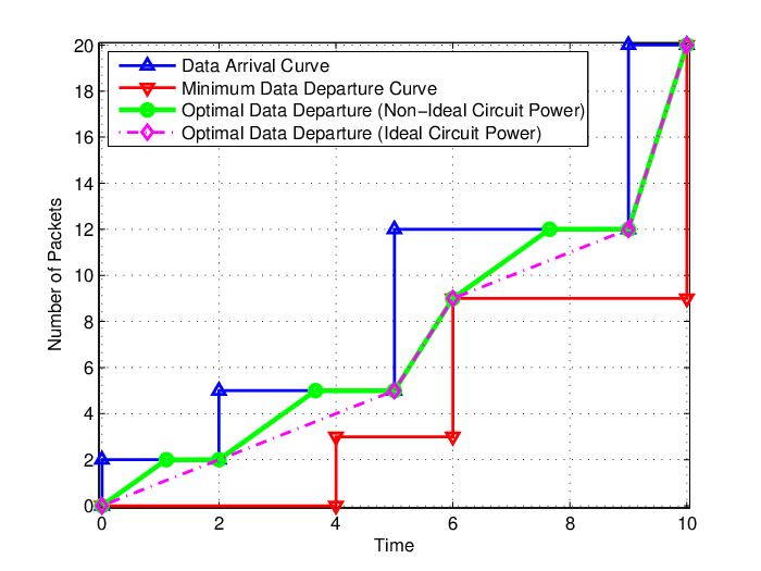
The optimal policy obtained by Algorithm 1 can be visualized by modifying the calculus approach in [9]. Define the data arrival and minimum departure curves and as:
| (16) |
where is the unit-step function: , if , and otherwise. In the ideal () circuit power case, the optimal transmission policy requires the transmitter to be always on, i.e. , [10, 12]. In this case, consider a piece-wise linear data departure curve:
| (17) |
where the rates per epoch serve as the piece-wise slopes for . Following [9], the optimal departure curve is shown to be the trajectory of letting a string tie its one end at the origin , pass the other end through , and then taut between and ; see Fig. 2. Consequently, the optimal for the ideal circuit power case can be derived from .
Interestingly, the optimal for the non-ideal circuit power case can be simply obtained by an -clipping process over . Specifically, we can set:
| (18) |
With (18), the corresponding optimal data departure curve under non-ideal circuit power is plotted in Fig. 2. Comparing to , the same amount of data departs per epoch in . Yet, different from , an on-off transmission strategy is adopted when for epoch . This is because the total energy cost for over such an epoch is in fact minimized by a transmission with over an “on” period of length , i.e.,
| (19) |
For the epoches with , however, any on-off strategy with and only increases the energy cost since
| (20) |
where the inequality is due to the fact that is strictly increasing when . Hence, the data departures over these epoches remain the same in and .
It is worth noting that the optimal transmission strategy is in fact not unique in the on-off transmission epoches. In an on-off period including e.g., epoch to epoch , different from computed in (18), we can have another set of such that . As long as are feasible, they are also optimal. In fact, we may even let (i.e., transmitter is “off”) for some epoches, while carrying out transmission only over the remaining epoches in an on-off period per Lemma 1.
III-D Development of Online Scheme
To obtain the optimal benchmark, we assumed a non-causal case where complete information about the packet arrivals during the time interval is available. When a-priori knowledge of the future packet arrivals is not available in practice, we can develop a heuristic online scheme based on the proposed optimal offline policy. The idea is to schedule the packet transmissions according to the optimal rate control policy based on the current packet arrivals, and reschedule when new packets arrive. For instance, suppose that packets arrive at time instant with (different) deadline requirements. We can construct the set in accordance to the deadline requirements, and let the set , where is determined by the largest deadline . With such a , we run the proposed Algorithm 1 to find the optimal transmission policy until new packets arrive at . Then we treat the current time instant as new “” instant, and update the set by subtracting all by , removing the past deadlines (i.e. with negative after subtraction), and then including the deadline requirements for the newly arriving packets. The set also needs to be updated. Note that we always have , where is updated as the sum of the remaining packets in the buffer and the newly arriving packets, and is determined by the last deadline in the updated . Algorithm 1 is run for the new , and the subsequent packet transmissions follow the resultant new policy. This process continues until all the packets are delivered.
IV Generalization to Time-Varying Channel
In this section, we generalize the proposed approach to a time-varying wireless channel, where the channel state in general changes with time. With a little abuse of notation, here we redefine an epoch as the interval between two consecutive channel or data state changing instants. Again, over the entire transmission interval , assume that there are (channel or data) state changing instants . There are epoches with length . The packet arrival process and deadline requirements are modeled by set and set . Let denote the channel coefficient at epoch ; and .
With the power function , we formulate the total energy consumption minimization problem over time-varying channels as follows:
| (21) |
With a change of variable , the non-convex problem in (21) can be also reformulated into a convex program for . Let collect the optimal Lagrange multipliers, and . Relying on the KKT conditions for the convex reformulation, we can follow the similar lines in Section III-A to derive the sufficient and necessary optimality conditions for (21):
| (22) |
| (23) |
| (24) |
For any , we can derive from (22) that
| (25) |
Let denote the first derivative of . We clearly have: , leading to , and . The latter is the celebrated water-filling form, where serves as a water-level.
Substituting into (22) implies:
| (26) |
For each per epoch, we can obtain an EE-maximizing rate in (14). Note that is different for different per epoch. As with Lemma 1, relying on (26), we can show that:
Lemma 3
The optimal transmission policy for (21) can only adopt one of the following three (“off”, “on-off” and “on”) strategies per epoch : (i) , (ii) , , or (iii) , .
As with Lemma 2, we can establish that:
Lemma 4
In the optimal policy for (21), the rates for epoches with are given by: , where the water-level can only increase after a where , and decrease after a where .
Similar to the time-invariant channel case, Lemma 3 states that the optimal policy depends on the EE-maximizing rates; i.e., any transmit-rate less than the EE-maximizing rate should not be adopted at epoch . However, the value of is in general different for different across epoches. In both time-invariant and time-varying channel cases, the change of “water-level” follows the same pattern: it increases after a casuality constraint becomes tight, and decreases after a deadline constraint is tight. Given the same , the same transmit-rate is maintained in the time-invariant case. This leads to the -clipped “string-tautening” procedure in Algorithm 1. For the time-varying channel case, the same water-level yields different transmit-power and rate when channel varies; specifically, higher rates are employed for better channels through a water-filling type power allocation for the most efficient energy usage. This revealed structure of the optimal policy implies that we can modify Algorithm 1 to implement a water-level based “string-tautening” approach to finding the optimal solution for (21).
To this end, let or denote the constant water-level to make the th causality or the th deadline constraint become tight at or . Given an invariant water-level before (or ), the optimal rate per epoch is given by if . Define:
| (27) |
Since we must have if per Lemma 3, we can have only when (recall that is an increasing function). With the water-level , the optimal strategy per epoch is then:
| (28) |
Define data departure per epoch . By (28), we have:
| (29) |
Using (29), the values of and can be calculated by solving the equations:
| (30) |
Note that and are increasing in ; see an example in Fig. 3. As a result, the equations in (30) can be solved by a bisectional search.

With and obtained, the optimal for (21) can be computed by a -clipped “water-tautening” approach in Algorithm 2.
Algorithm 2 -Clipped “Water-Tautening”
The key component in Algorithm 2 is the function FirstChangeW, which determines the first water-level changing time and the water-level used before . The two candidate water-levels are updated as: and , which are in fact the maximum and minimum values for an invariant water-level to satisfy all the causality and deadline constraints before , respectively; and , are the corresponding or yielding , . If we have at a certain , then the water-level needs to be changed before since no invariant water-level can satisfy all the causality and deadline constraints so far. The first water-level changing time can be obtained by comparing and to see which type of constraint first becomes tight. When the returned , Function FirstChangeW can be reused for a new system over the remaining time to find the next water-level changing time and the next water-level. Note that Function FirstChangeW also returns the delivered data amount before , which is necessary for determining the length of the “on” period for the possible on-off epoch with .
As with Theorem 1, we can establish that:
Theorem 2
Algorithm 2 computes the optimal transmission policy for (21) with a linear complexity .
V Numerical Results

Consider packet transmission over seconds and the number of total packet arrivals is . The bandwidth for the system is KHz while each packet contains K bits. The power-rate relationship is dictated by the Shannon-capacity formula in (1). The non-zero circuit power during the “on” mode is Watts. (i) Assume first a time-invariant channel with power gain and unit noise variance. To validate the proposed Algorithm 1, we use it and the standard CVX toolbox to solve (3) when the transmission interval , , , , , seconds. For each value, we test trial cases where the intervals and follow a uniform distribution with mean , respectively. It is confirmed that the two methods yield the same rate control policies for all trial cases, demonstrating the correctness of the proposed Algorithm 1. On the other hand, since Algorithm 1 directly constructs the optimal solution for the problem at hand relying on the optimality conditions, it is much more efficient than the CVX toolbox in terms of computational complexity. Fig. 4 depicts the average CPU time required for the two methods. We can observe that the required CPU time of the proposed Algorithm 1 is less than 0.01% of that of the standard CVX toolbox for all values. (ii) Consider next a time-varying channel where the random channel coefficients per second are independently generated from a Rayleigh distribution with average power . We use Algorithm 2 and the standard CVX toolbox to solve (21). Again, it is confirmed that Algorithm 2 and the CVX toolbox yield the same rate control policies for all trial cases. Fig. 4 also includes the average required CPU time with these two methods. It is observed that Algorithm 2 only requires a CPU time less than 0.1% of that with the CVX toolbox for all values. The significantly reduced complexity can clearly benefit the real-time implementation of the algorithm in e.g., the proposed online scheme.

Next, in terms of energy consumption, we compare the optimal policies obtained by our proposed Algorithm 1 and its online scheme (as described in Section III-D), as well as two heuristic policies in the time-invariant channel case. Heuristic 1 is obtained by always selecting a rate to meet the next active causality or deadline constraint with equality. Heuristic 2 is obtained by using the calculus approach in [9] under an ideal circuit-power assumption, even though the circuit-power consumption is in fact non-ideal. Both heuristic approaches can provide a feasible policy that satisfies all the causality and deadline constraints in (3) for fair comparison. Fig. 5 provides the average energy consumption with the policies obtained by Algorithm 1 and the two heuristic approaches, when , and seconds. Again, for each value, we test 50 trial cases where the causality and deadline constraints are randomly generated. The proposed Algorithm 1 significantly outperforms the two heuristic counterparts, always yielding the smallest energy consumption for every value. Compared to the heuristic policies, the energy saved from the optimal policy becomes more significant as the value of increases, i.e., as the entire transmission interval becomes longer. For small values, Heuristic 2 has approximately the same performance as the proposed Algorithm 1. The reason is that the constraints are usually strict and thus the optimal transmit-rates are usually larger than when value is small; as a result, in the optimal transmission policy produced by Algorithm 1, there are very few on-off epoches, i.e. the transmitter is always selected to be on, rendering the policies by Algorithm 1 and Heuristic 2 become almost identical. For large values, Heuristic 2 scheme becomes almost the same as the naive Heuristic 1. The optimal policy can save up to 100 times the energy over the naive Heuristic 1 for small , and can save times the energy over the heuristic ones for large . It is also observed that the energy consumption of the proposed online scheme is close to that of the optimal offline strategy, especially for large . In such a case, even the proposed online scheme without the knowledge of future arrivals can save almost times the energy over the heuristic ones with complete a-priori information about the packet arrivals.
Lastly, we compare the energy consumption between the proposed Algorithm 2, Heuristic 1 and 2, as well as another heuristic method (called Heuristic 3) in the time-varying channel case. Specifically, Heuristic 3 is obtained by using Algorithm 1 under a time invariant channel assumption, even though the channel is in fact time-varying. Fig. 6 shows the energy consumption of these schemes, where each result is averaged over 50 random trials. The proposed Algorithm 2 apparently outperforms the heuristic counterparts, always yielding the smallest energy consumption for each trial case. It is observed that the optimal policy obtained by our Algorithm 2 can save up to 100 times the energy over Heuristic 1 and 2, and 5 times the energy over Heuristic 3, especially for large values.

VI Conclusion
We proposed a novel unified approach to optimizing the energy-efficient transmission policy for delay-limited bursty packet arrivals under non-ideal circuit power consumption. Efficient algorithms were developed to find the optimal offline solutions with a low computational complexity for both time-invariant and time-varying channels. An insightful visualization was presented to reveal the specific structure of the optimal policy. Our approach can provide the optimal benchmarks for practical schemes. Based on the proposed optimal offline policies, development of energy-efficient online scheduling policies was also discussed and will be further explored in our future work. Generalization of our approach to wireless networks with multiple interfering links will be also pursued.
-A Proof of Lemma 1
Define . Taking the first derivative of , we have:
| (31) |
Due to its “convex-over-linear” form, we can show that first decreases and then increases with , and it reaches the minimum at . This implies:
| (32) |
If we have an when , it follows from (32) that . But when , (13) implies that , which leads to a contradiction. Hence, is not allowed when .
-B Proof of Lemma 2
Clearly, changes only when changes its value. By the definition , if , , and , , then a constant will be used over all the epoches. We will have a change only when for a certain , or for a certain , which occurs at the corresponding or . In addition, it follows from the complementary slackness conditions (10)–(11) that we must have or at such a or .
If a change occurs at a certain , then . For the epoch , we have ; thus . On the other hand, for the epoch , we have ; thus . Therefore, ; consequently, the rate increases after since is an increasing function of .
If a change occurs at a certain , then . For the epoches and , we can similarly derive that ; consequently, the rate decreases after .
-C Proof of Theorem 1
Due to the rules used in the function FirstChangeR, it can be shown that the rate-changing pattern in the transmission policy produced by Algorithm 1 is consistent with the optimal structure revealed in Lemma 2, i.e., (i) if the rate in use is first and then changed to at where , then we must have ; and (ii) if the rate is changed at where , then we must have the next rate . Fig. 7 provides an illustration and the sketch of the proof for this claim.
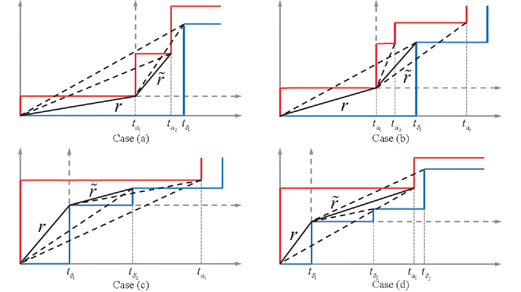
Suppose that the rate changes times in yielded by Algorithm 1. We divide the policy into phases: rate over epoches , over epoches , , over epoches . We can then construct a set of Lagrange multipliers as follows:
Let , where the inequality is due to the strictly increasing of , leading to positivity of . Let , if for a certain and , or let , if for a certain and , . We have shown that the rate if the causality constraint is tight at , or if the deadline constraint is tight at . Recalling that is increasing in , it readily follows that or , depending on which type of constraint is tight at . Except these positive and or , all other Lagrange multipliers in are set to zero.
With such a , the complementary slackness conditions (10)–(11) clearly hold. Using such a also leads to , (with and ). This implies that , . In addition, the construction of ensures when , and computes a feasible set of when in each phase . This guarantees that each pair of satisfies (9); thus, follows the optimal structure in Lemma 1.
We have proven that yielded by Algorithm 1 and the Lagrange multipliers constructed accordingly, satisfy the sufficient and necessary optimality conditions (9)–(11) for (3). It then readily follows that is a global optimal policy for (4). In the search of the rate-changing points and the associated rates in Algorithm 1, we only need to go through the data arrival or deadline time instants as shown in Fig. 2; hence, the algorithm has a complexity .
References
- [1] Z. Nan and X. Wang, “Energy-efficient transmission of delay-limited bursty data packets under non-ideal circuit power consumption,” in Proc. ICC, Sydney, Australia, Jun. 2014.
- [2] Z. Nan, T. Chen and X. Wang, “Energy-efficient transmission of delay-limited bursty data packets over time-varying channels under non-ideal circuit power,” in Proc. ChinaSIP, Xi’an, China, July 2014.
- [3] R. Berry and R. Gallager, “Communication over fading channels with delay constraints,” IEEE Trans. Inf. Theory, vol. 48, no. 5, pp. 1135–1149, May 2002.
- [4] E. Uysal-Biyikoglu and A. E. Gamel, “On adaptive transmission for energy efficient in wireless data networks,” IEEE Trans. Inf. Theory, vol. 50, no. 12, pp. 3081–3094, Dec. 2004.
- [5] A. El Gamal, C. Nair, B. Prabhakar, E. Uysal-Biyikoglu, and S. Zahedi, “Energy-efficient scheduling of packet transmissions over wireless networks,” in Proc. INFOCOM, vol. 3, pp. 1773–1783, 2002.
- [6] Y. Yao and G. B. Giannakis, “Energy-efficient scheduling for wireless sensor networks,” IEEE Trans. Commun., vol. 53, no. 8, pp. 1333–1342, Aug. 2005.
- [7] X. Wang and G. Giannakis, “Power-efficient resource allocation for time-division multiple access over fading channels,” IEEE Trans. Inf. Theory, vol. 54, no. 3, pp. 1225–1240, Mar. 2008.
- [8] E. Uysal-Biyikoglu, B. Prabhakar, and A. El Gamal, “Energy-efficient packet transmission over a wireless link,” IEEE/ACM Trans. Netw., vol. 10, no. 4, pp. 487–499, Aug. 2002.
- [9] M. Zafer and E. Modiano, “A calculus approach to minimum energy transmission policies with quality of service guarantees,” in Proc. INFOCOM, vol. 1, pp. 548–559, 2005.
- [10] W. Chen, M. Neely, and U. Mitra, “Energy-efficient transmissions with individual packet delay constraints,” IEEE Trans. Inf. Theory, vol. 54, no. 5, pp. 2090–2109, May 2008.
- [11] W. Chen, U. Mitra, and M. Neely, “Energy-efficient scheduling with individual packet delay constraints over a fading channel,” Wireless Netw., vol. 15, no. 5, pp. 601–618, 2009.
- [12] X. Wang and Z. Li, “Energy-efficient transmissions of bursty data packets with strict deadlines over time-varying wireless channels,” IEEE Trans. Wireless Commun., vol. 12, no. 5, pp. 2533–2543, May 2013.
- [13] J. Xu and R. Zhang, “Throughput optimal policies for energy harvesting wireless transmitters with non-ideal circuit power,” to appear in IEEE J. Sel. Areas Commun..
- [14] Q. Bai, J. Li, and J. Nossek, “Throughput maximizing transmission strategy of energy harvesting nodes,” in Proc. IWCLD, 2011.
- [15] O. Orhan, D. Gunduz, and E. Erkip, “Throughput maximization for an energy harvesting system with processing cost,” in Proc. ITW, 2012.
- [16] O. Blume, H. Eckhardt, S. Klein, E. Kuehn, and W. M. Wajda, “Energy savings in mobile networks based on adaptation to traffic statistics,” Bell Labs Tec. J., vol. 15, no. 2, pp. 77–94, Sep. 2010.
- [17] G. Miao, N. Himayat, and G. Li, “Energy-efficient link adaptation in frequency-selective channels,” IEEE Trans. Commun., vol. 58, no.2, pp. 545–554, Feb. 2010.
- [18] S. Boyd and L. Vandenberghe, Convex Optimization, Cambridge University Press, 2004.
- [19] X. Wang and G. Giannakis, “Resource allocation for wireless multiuser OFDM networks,” IEEE Trans. Inf. Theory, vol. 57, no. 7, pp. 4359–4372, July 2011.
- [20] M. Grant and S. Boyd, CVX: Matlab software for discplined convex programming, http://cvxr.com/cvx/, Oct. 2010.