Proof of a refinement of Blum’s conjecture on hexagonal dungeons

A lattice partitions the plane into fundamental regions. A (lattice) region considered in this paper is a finite connected union of fundamental regions. We call the union of any two fundamental regions sharing an edge a tile. We would like to know how many different ways to cover a region by tiles so that there are no gaps or overlaps; and such coverings are called tilings. We use the notation $\operatorname{M}(R)$ for the number of tilings of a region $R$, and $\mathcal{M}(R)$ for the set of all tilings of $R$.

Consider the lattice obtained from the triangular lattice by drawing in all attitudes of each unit triangle. The resulting lattice is usually called $G_{2}$-lattice, since it is the lattice corresponding to the affine Coxeter group $G_{2}$. On the $G_{2}$-lattice, Blum investigated a variation of Aztec dungeon (see [1]) called hexagonal dungeon. In particular, we draw a hexagonal contour of side-lengths¹¹ 1 The unit here is the side-length of the unit triangles. $a,2a,b,a,2a,b$ (in cyclic order, start by the west side) as the light bold contour in Figure 1.1. We draw next a jagged boundary running along the hexagonal contour (see the dark bold closed path in Figure 1.1), and denote by $HD_{a,2a,b}$ the region restricted by the boundary. Blum found a striking pattern of the numbers of tilings of the hexagonal dungeons, which led him to his well-known conjecture that the hexagonal dungeon $HD_{a,2a,b}$ has $13^{2a^{2}}14^{\lfloor\frac{a^{2}}{2}\rfloor}$ tilings, when $b\geqslant 2a$. Fourteen years latter, Ciucu and the author proved the conjecture in [2] by using Kuo’s graphical condensation method [4]. However, the proof did not explain the (surprising) appearance of the numbers 13 and 14 in the Blum’s formula. In this paper, we consider generating function of the tilings of the hexagonal dungeons and give an explanation for the appearance of the numbers $13$ and $14$.

The tiles in a hexagonal dungeon have three possible shapes: an obtuse triangle, an equilateral triangle, and a kite (see Figure 1.2). We consider the following generating functions

where $m$, $n$, $l$ are respectively the numbers of obtuse triangle tiles, equilateral triangle tiles, and kite tiles in the tiling $T$ of $HD_{a,2a,b}$. We call $F(x,y,z)$ the tiling generating function of the hexagonal dungeon. Our goal is to prove the following refinement of Blum’s conjecture.

This paper is organized as follows. In Section 2, we recall the definition of two important regions $D_{a,b,c}$ and $E_{a,b,c}$, which were first introduced in [2]. In addition, we state a result on their tiling generating functions (see Theorem 2.1), which is the key to prove Theorem 1.1. Next, we prove Theorem 2.1 in Section 3, and use this to prove Theorem 1.1 in Section 4. Section 5 uses Theorem 1.1 to enumerate of tilings of several new types of hexagonal dungeons. Finally, Section 6 is devoted for an open problem on hexagonal dungeons with defects.

First, we recall briefly the definition of the two regions $D_{a,b,c}$ and $E_{a,b,c}$, which were first introduced in [2].

Let $a,b,c,d,e,f$ be six non-negative integers. Starting from a vertex of some unit triangle on $G_{2}$-lattice, we travel along lattice lines $a$ units southwest, $b$ units southeast, $c$ units north, $d$ units northeast, and $e$ units northwest. We adjust $e$ so that the ending point is on the same vertical line as the starting point. Finally, we close the contour by go $f$ units north or south.

The contour is illustrated in Figure 2.1, for the case $a>c+d$; and in Figure 2.2, for the case $a\leqslant c+d$. If some side of the contour has length $0$, we assume that the side shrinks to a point. Denote by $\mathcal{C}(a,b,c)$ the resulting contour.

Based on the contour $\mathcal{C}(a,b,c)$, we define two lattice regions $D_{a,b,c}$ and $E_{a,b,c}$ determined by the dark jagged boundaries as in Figure 2.1, for the case $a>c+d$, and by Figure 2.2, for the case $a\leqslant c+d$.

We already showed in [2] that the closure of the contour $\mathcal{C}(a,b,c)$, the choice of $e$, and the existence of tilings in the regions $D_{a,b,c}$ and $E_{a,b,c}$ require $b\geqslant 2$, $d=2b-a-2c$, $e=b+d-a=3b-2a-2c,$ and $f=|a-c-d|=|2a+c-2b|$. Moreover, it has been shown in [2] that the numbers of tilings of $D_{a,b,c}$ and $E_{a,b,c}$ is given by powers of $13$ and $14$ (see Theorem 3.1).

Next, we consider the tiling generating functions of $D_{a,b,c}$ and $E_{a,b,c}$ as follows. Define

where $m$ and $n$ are respectively the numbers of obtuse triangle tiles and equilateral triangle tiles in tiling $T$ of $D_{a,b,c}$. Similarly, we set

where $k$ and $l$ are the numbers of obtuse triangle tiles and equilateral triangle tiles in tiling $T^{\prime}$ of $E_{a,b,c}$.

Define three new functions as follows:

and

Denote by $P(x,y,z)$ and $Q(x,y,z)$ the two polynomials appearing in Theorem 1.1, i.e.

and

In addition, we define two simple functions $h(a,b,c)$ and $p(a,b,c)$ as

and

The generating functions $\Phi(a,b,c)$ and $\Psi(a,b,c)$ are given by the theorem stated below.

Theorem 2.1 is the key in proving our main Theorem 1.1 in Section 4.

We conclude this section by noticing that Ciucu proved implicitly the formulas of $\Phi(n,n,0)$ and $\Psi(n,n,0)$ (under the form of tiling generating functions of the Aztec dungeons in Theorem 3.1 and Proposition 3.6 of [1]). In other word, our Theorem 2.1 generalizes Ciucu’s Theorem 3.1 and Proposition 3.6 in [1].

Before proving Theorem 2.1, we need several definitions and terminology as follows.

A perfect matching of a graph $G$ is a collection of disjoint edges covering all vertices of $G$. The dual graph $G$ of $R$ is the graph whose vertices are fundamental regions in $R$ and whose edges connect precisely two fundamental regions sharing an edge. The tilings of a region can be identified with the perfect matchings of it dual graph. In the view of this, we use the notation $\operatorname{M}(G)$ for the number of perfect matchings of $G$.

In the weighted case, $\operatorname{M}(G)$ defines the sum of weights of perfect matchings of $G$, where the weight of a perfect matching is the product of weights of all constituent edges. Define similarly the weighted sum $\operatorname{M}(R)$ of tilings of a weighted region $R$. Each edge of the dual graph $G$ of $R$ has the same weight as that of its corresponding tile in $R$.

Consider the following recurrences (R1)–(R5), where the notations $\bigstar(a,b,c)$ and $\lozenge(a,b,c)$ have been used to indicate some polynomials in $\mathbb{Z}[x,y]$.

We notice that the recurrence (R1) implies the recurrence in Lemmas 4.1 and 5.1 in [2] by specializing $x=y=1$. Similarly, (R2) and (R3) are weighted versions of the recurrence in Lemmas 4.2(a) and 5.2(a) and the recurrence in Lemmas 4.2(b) and 5.2(b) in [2], respectively. Finally, the $x=y=1$ specializations of (R4) and (R5) give the recurrences in Lemmas 4.3 and 5.3 of [2].

Next, we show that $\Phi(a,b,c)$ and $\Psi(a,b,c)$ satisfy the above recurrences (R1)–(R5) (with certain constraints) by using the following Kuo’s Condensation Theorem.

One readily sees that Lemma 3.2 implies Lemma 4.1 in [2] by specializing $x=y=1$.

Applying also the Kuo’s Theorem 3.1 to the dual graphs of $D_{a,b,c}(x,y)$ and $E_{a,b,c}(x,y)$ with the four vertices $u,u,w,t$ chosen as in Figure 3.3, we get the following weighted version of Lemma 4.2 in [2].

A similar generalization of Lemma 4.3 in [2] is obtained by applying Kuo condensation to the dual graphs of $D_{a,b,c}(x,y)$ and $E_{a,b,c}(x,y)$ with the four vertices $u,v,w,t$ selected as in Figure 3.4.

We now denote by $\phi(a,b,c)$ and $\psi(a,b,c)$ the expressions on the right hand sides of the equalities (2.10) and (2.11) in Theorem 2.1, respectively. It is routine to verify that the two functions $\phi(a,b,c)$ and $\psi(a,b,c)$ satisfy the same recurrences (R1)–(R5) for any $a,b,c\in\mathbb{Z}$ (If one wants a detailed verification, we recommend the proofs of Lemmas 5.1–5.3 in [2]). This yields an inductive proof of Theorem 2.1 on the perimeter of the contour $\mathcal{C}(a,b,c)$.

The base cases are the situations when at least one of the following hold:

1. (1)

   Perimeter of the contour if at most 14.

2. (2)

   $b\leqslant 4$.

3. (3)

   $c+d=2b-a-c\leqslant 2$.

Similar to the proof of Theorem 3.1 in [2]. These base cases can be verified by the help of the computer package vaxmacs written by David Wilson²² 2 This software is available at http://dbwilson.com/vaxmacs/, together with Maple by Maplesoft.

For induction step, we assume that the theorem is true for any regions $D_{a,b,c}(x,y)$ and $E_{a,b,c}(x,y)$ with perimeter greater than or equal to $16$ (it is easy to check that the perimeter is always even). We consider several cases ans show that the number of tilings of the regions and the expressions on the right hand sides of (2.10) and (2.11) satisfy the same recurrence: (R1), (R2), $\dots$ or (R5). However, all arguments here are essentially the same as that in the induction step of the proof of Theorem 3.1 in [2] (with the recurrences are replaced by their corresponding weighted versions). Therefore, we can finish our proof of Theorem 2.1 here.

Before presenting the proof of Theorem 1.1, we quote the following lemma.

In this section, we investigate several new hexagonal dungeons.

The $G_{2}$-lattice can be partitioned into rhombi with two diagonals drawn in (see the top picture in Figure 5.1). Apply the replacing rule (a) in Figure 5.1 to all the rhombi, and denote by $G_{2}^{(1)}$ the resulting lattice. We have a variant of the hexagonal dungeon $HD_{a,2a,b}$ as in Figure 5.2 (see the region restricted by the dark bold jagged contour). Denote by $HD^{(1)}_{a,2a,b}$ the new hexagonal dungeon.

Next, we quote a well-known subgraph replacement trick called urban renewal, which was first discovered by Kuperberg.

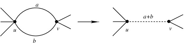
We have a small observation as follows. If there are several parallel edges connecting the same vertices $u$ and $v$ in a graph $G$, then the number of perfect matchings of $G$ doesn’t change if the we can replace these parallel edges by a new single edge connecting $u$ and $v$ with the weight equal to the sum of weights of the original edges (see Figure 5.4).

Next, we consider the application of the replacement rule (b) in Figure 5.1 to all rhombi of $G_{2}$-lattice, and denote by $G_{2}^{(2)}$ the resulting lattice. On the $G_{2}^{(2)}$-lattice, we have a new version of the hexagonal dungeons illustrated by the region restricted by the dark bold contour in Figure 5.6.

References

- [1] M. Ciucu, Perfect matchings and perfect powers, J. Algebraic Combin. 17 (2003), 335–375.
- [2] M. Ciucu and T. Lai, Proof of Blum’s Conjecture on Hexagonal Dungeons, J. Combin. Theory Ser. A 125 (2014), 273–305.
- [3] N. Elkies, G. Kuperberg, M. Larsen, and J. Propp, Alternating-sign matrices and domino tilings (Part I), J. Algebraic Combin. 1 (1992), 111–132.
- [4] E. H. Kuo, Applications of Graphical Condensation for Enumerating Matchings and Tilings, Theor. Comput. Sci. 319 (2004), 29–57.
- [5] T. Lai, Enumeration of hybrid domino-lozenge tilings, J. Combin. Theory Ser. A 122, 2014, 53–81.
- [6] J. Propp, Enumeration of matchings: Problems and progress, New Perspectives in Geometric Combinatorics, Cambridge Univ. Press, 1999, 255–291.