Spatial Performance Analysis and Design Principles for Wireless Peer Discovery

Several studies have suggested aggressive schemes where each peer can transmit its unique signal and simultaneously receive multiple signatures from other peers for rapid and collision-free peer discovery, e.g., [7, 8], but a simple random access protocol is still regarded as the basis of wireless peer discovery [9, 10, 11, 12, 13, 14, 15, 16] because the lack of a priori information about peers in dynamic wireless networks may only provide the uncoordinated sharing of peer discovery resources among peers.

The primary reason for performance degradation in a random access protocol is packet collisions due to the simultaneous transmission of peers; thus, several studies have investigated the quantification and improvement of the peer discovery performance based on the packet collision model [9, 10, 11]. However, this collision model oversimplifies wireless receiving operations. In fact, the success or failure of packet reception is primarily determined by the physical layer metrics, e.g., SINR, rather than whether or not packets simply collide. In addition, the requirement of this received SINR depends on the physical transceiving scheme, such as the receiver structure and level of modulation and coding scheme (MCS). Based on this, there have been attempts to understand the effect of physical layer characteristics including the receiver structure and wireless channel [12, 13]. In [12], a joint iterative decoding method for multiuser detection was applied to peer discovery but its system performance improvement was only evaluated using simulation. The work of [13] analyzed the performance of multipacket reception based on the conventional packet collision model. These approaches remains insufficient to reveal the implications of the randomness of wireless channels and peer locations.

There have also been recent studies that analyze the spatial performance by statistically modeling peer location and wireless channel [14, 15, 16]. In [14], the received power of the signals from randomly located peers was modeled in a probabilistic manner and the multipacket reception capability was assumed. However, the performance was only expressed in a form with as many cumbersome integrations as the number of peers; therefore, this result could not explicitly present the design implications of wireless peer discovery. In contrast, the works of [15, 16] attempted to mathematically analyze the peer discovery performance with interference considerations using a stochastic geometry framework [4, 5, 6]. The work of [15] compared the packet collision and SINR models when peers were distributed according to a homogeneous Poisson point process (PPP), and it expressed the average number of discovered peers in a closed form under the Rayleigh fading channel when the noise power can be ignored. A similar result was also presented in [16]. The results under this specific channel model, i.e., the Rayleigh fading with zero noise power, provide a basis for the analysis under channel models that belong to the exponential family, e.g. the Nakagami-$\displaystyle m$ fading channel [17]. However, the explicit derivation of the performance under more general channel models, such as incorporating the Nakagami-$\displaystyle m$ fading channel, nonzero background noise power, and shadowing, also has the significant merit because it enables the clarification of the relationship between wireless channels and discovery operation parameters, which leads to the design principles for the key operation parameters including the transmission probability for a half duplex operation, received SINR requirement, and transmit power under various channel environments. This extension was not considered in [15] and [16].

This paper investigates wireless peer discovery with respect to the mean number of successfully discovered peers, which is denoted by $\displaystyle\mathbb{E}\{S\}$, by comprehensively considering the wireless properties as well as the discovery operation properties. The main contributions are highlighted into the following three aspects.

This paper considers the multichannel random hello protocol for wireless peer discovery illustrated in Fig. 1 when peers or nodes¹¹ 1 In this paper, both the terms are used synonymously. are randomly distributed in a two-dimensional space. The model assumes resource orthogonality, i.e., signals transmitted over different resources do not interfere with each other. The premise for this orthogonality is global synchronization [19]. If nodes are not precisely time synchronized, the interference that results from time mismatches may significantly degrade the performance. However, in general, the time synchronization in distributed wireless networks is a resource and energy intensive task. External signals from the existing infrastructure, e.g. nearby cellular base stations, may render this difficult task simpler [19, 20]; such signals are exploited as timing reference signals for rough synchronization, and then the remaining time offsets are further corrected through additional synchronization procedures among the nodes in order that the residual timing errors can be readily accommodated in the signal level, e.g., using cyclic prefix (CP) in OFDMA systems. Accordingly, this paper assumes that all nodes are time synchronized and does not consider performance degradation due to time mismatches. The model also assumes that all nodes operate in a half duplex manner. For this half duplex operation, a node decides whether it transmits or receives a hello packet identifying a node every time slot in a probabilistic manner, and $\displaystyle\rho$ denotes the probability that a node transmits in a time slot, i.e., the transmission probability.

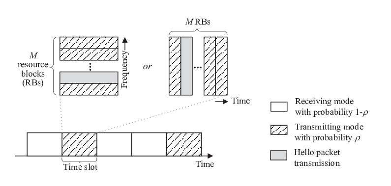
One time slot consists of $\displaystyle M$ resource blocks (RBs) in a frequency or time domain, and one RB is used for a hello packet transmission. For peer discovery, nodes in the transmitting mode broadcast their hello packet using one RB randomly chosen among $\displaystyle M$ RBs while nodes in the receiving mode try to detect the packets simultaneously over all $\displaystyle M$ RBs in a time slot. Let $\displaystyle\xi>0$ denote the minimum received SINR required for the successful reception of a packet. If a node in the receiving mode receives a hello packet with SINR above $\displaystyle\xi$, then it means that this node successfully discovers the node that transmits the packet. Note that the value of $\displaystyle\xi$ determines the MCS level at which a hello packet is transmitted.

The model assumes that the nodes are spatially distributed according to a homogeneous PPP with node density $\displaystyle\lambda$, which is denoted by $\displaystyle\Phi$. In order to investigate the node average performance, the performance of a reference receiving node is observed and such a node is referred to as a typical node. A typical node is assumed to be located at the origin and search potential target node $\displaystyle i$ in a time slot. If node $\displaystyle i$ is transmitting in the same time slot, the signal transmitted by node $\displaystyle i$ becomes the desired signal of a typical node. Assume that node $\displaystyle i$ transmits a hello packet using the $\displaystyle m$th RB in the time slot. Under these assumptions, all signals sent over the $\displaystyle m$th RB by nodes in the transmitting mode, other than node $\displaystyle i$, become interference. Note that a typical node is interested in hello packets from all other nodes; thus, target node $\displaystyle i$ indicates an arbitrary node rather than a specific node. Therefore, according to Slivnyak’s theorem [21], nodes except a typical node and the target node $\displaystyle i$ still constitute a homogeneous PPP with the same density as $\displaystyle\lambda$. These nodes are potential interferers. Let $\displaystyle\Phi_{q}$ denote a homogeneous PPP with density $\displaystyle\lambda q$ that results from the independent thinning of homogeneous PPP $\displaystyle\Phi$ with retention probability $\displaystyle q$. In a given time slot, each node is transmitting with probability $\displaystyle\rho$ and it uses the same RB as that of node $\displaystyle i$ with probability $\displaystyle 1/M$. Thus, the spatial distribution of the interfering nodes can be modeled as the thinning of an original PPP with a retention probability $\displaystyle\rho/M$, and it is expressed as a homogeneous PPP with density $\displaystyle\lambda\rho/M$, i.e., $\displaystyle\textstyle\Phi_{\rho/M}$. In fact, each node in $\displaystyle\textstyle\Phi_{\rho/M}$ becomes both a potential target node and a interferer of a typical node. $\displaystyle X_{j}$ denotes the location of node $\displaystyle j$ and $\displaystyle|X_{j}|$ represents the distance from the origin to $\displaystyle X_{j}$. Assume that all nodes have the same transmit power $\displaystyle p$. The standard power loss propagation model with the path loss exponent of $\displaystyle\alpha$ ($\displaystyle>2$) is supposed. Let $\displaystyle h_{i}$ and $\displaystyle g_{j}$ denote the fading power gains²² 2 They may denote the channel power gain including the shadowing as well as the Nakagami-$\displaystyle m$ or Rayleigh fading, depending on the wireless channel model. that the desired signal from node $\displaystyle i$ and the interfering signal from node $\displaystyle j$ undergo, respectively. It is assumed that $\displaystyle\{h_{i}\}$ and $\displaystyle\{g_{j}\}$ are independently and identically distributed (i.i.d.), respectively. Fig. 2 explains the spatial model considered in this paper.

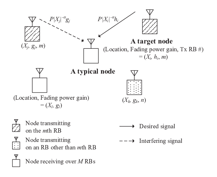
Eventually, when $\displaystyle\Xi(X_{i})$ denotes the received SINR at a typical node for the hello packet transmitted by a target node located on $\displaystyle X_{i}$,

where $\displaystyle\textstyle\sigma^{2}\triangleq\frac{\tilde{\sigma}^{2}}{p}$ and $\displaystyle\tilde{\sigma}^{2}$ denotes the noise power. Herein, $\displaystyle\textstyle\frac{1}{\sigma^{2}}=\frac{p}{\tilde{\sigma}^{2}}$ can be understood as the average received signal to noise ratio (SNR) at a unit distance, i.e., when $\displaystyle|X_{i}|=1$.

In this paper, wireless peer discovery aims to find as many nodes as possible, i.e., to maximize the average number of successfully discovered nodes. The successful peer discovery requires the fulfillment of the following three conditions: (i) a typical node is in the receiving mode; (ii) a target node is in the transmitting mode; and (iii) a hello packet that the target node transmits should be received with an SINR above $\displaystyle\xi$ at a typical node. The status of node $\displaystyle j$ is represented by $\displaystyle Z_{j}$, i.e., $\displaystyle Z_{j}=0$ if node $\displaystyle j$ is in the receiving mode and $\displaystyle Z_{j}=1$ otherwise. Let $\displaystyle P(X|Z_{0}=0)$ denote the probability that a typical node successfully discovers a target node located on $\displaystyle X$ when a typical node is in the receiving mode. Then, $\displaystyle P(X|Z_{0}=0)$ is given by

This success probability depends on the wireless channels and spatial distribution of the nodes, thus $\displaystyle P(X|Z_{0}=0)$ is expressed as a function of wireless channel parameters and node density $\displaystyle\lambda$ as well as discovery operation parameters including $\displaystyle M$, $\displaystyle\xi$, $\displaystyle\rho$, and $\displaystyle p$.

This paper considers wireless channel models that embrace shadowing as well as Nakagami-$\displaystyle m$ fading. That is, the fading power gain is given by the product of the gains that result from the shadowing and Nakagami-$\displaystyle m$ fading. The Nakagami-$\displaystyle m$ fading model does not only generalize or approximate various useful fading channels such as the Rayleigh and Rician fading channels, but it also allows a closed form of $\displaystyle\mathbb{E}\{S\}$ in some specific cases, e.g., when $\displaystyle\sigma^{2}=0$, where $\displaystyle\mathbb{E}\{S\}$ denotes the average number of nodes that a typical node successfully discovers over $\displaystyle M$ RBs. This is derived in the following sections. In addition, the results yielded in this Nakagami-$\displaystyle m$ fading model can be readily extended to those for wireless channel models that incorporate shadowing as long as the shadowing of links is i.i.d. [18, 22]. Therefore, the mathematical analysis in Sections III and IV concentrates on the Nakagami-$\displaystyle m$ fading and Rayleigh fading without shadowing. Then, the results will be extended to those for more general wireless channel models that incorporate shadowing.

When the Nakagami-$\displaystyle m$ fading model is only considered, the fading power gain $\displaystyle h$ follows the Gamma distribution and its complementary cumulative distribution function (ccdf) is given as follows:

where $\displaystyle m$ is the Nakagami-$\displaystyle m$ fading parameter. Under this Nakagami-$\displaystyle m$ fading channel model, the following lemma is a start toward deriving a simple form of $\displaystyle\mathbb{E}\{S\}$.

When $\displaystyle\sigma^{2}=0$, from Lemma II.1, the following results are obtained.

In (5), $\displaystyle\mathbb{E}\{S\}$ is determined by both the wireless channel parameters, e.g., $\displaystyle m_{s}$, $\displaystyle m_{i}$, and $\displaystyle\alpha$, and the discovery operation parameters, e.g., $\displaystyle M$, $\displaystyle\xi$, and $\displaystyle\rho$. This subsection elaborates on the design of the three discovery operation parameters. The design aims to maximize $\displaystyle\mathbb{E}\{S\}$ in (5). It is trivial to derive the optimal value of $\displaystyle\rho$ for maximizing $\displaystyle\mathbb{E}\{S\}$, which is denoted by $\displaystyle\rho^{*}$, i.e., $\displaystyle\textstyle\rho^{*}\triangleq\arg\max_{0<\rho<1}\mathbb{E}\{S\}$. $\displaystyle\rho^{*}$ always approaches zero regardless of $\displaystyle M$ and $\displaystyle\xi$. Therefore, the design of $\displaystyle M$ and $\displaystyle\xi$ can be separated from that of $\displaystyle\rho$, when $\displaystyle\sigma^{2}=0$. The meaning of $\displaystyle\rho^{*}$ will be discussed in more detail at the end of this subsection.

When $\displaystyle\xi$ is given, $\displaystyle\mathbb{E}\{S\}$ in (5) increases linearly with $\displaystyle M$. That is, regarding maximizing $\displaystyle\mathbb{E}\{S\}$ in (5), for a fixed $\displaystyle\xi$, $\displaystyle M$ can be designed regardless of the wireless channel parameters and $\displaystyle\rho$. However, the design of $\displaystyle M$ is highly correlated with that of $\displaystyle\xi$. As mentioned in Section II-A, the value of $\displaystyle\xi$ determines the MCS level, i.e., the data rate, available for a hello packet transmission. When the total amount of peer discovery resources are fixed, the data rate decided by $\displaystyle\xi$ affects how many RBs the total resources can be divided into, thus $\displaystyle M$ and $\displaystyle\xi$ should be jointly designed.

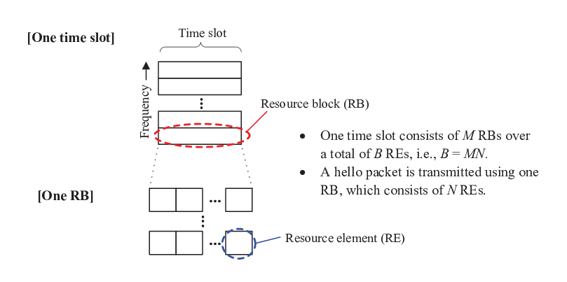
The joint design begins with quantifying the relationship between $\displaystyle M$ and $\displaystyle\xi$. Typically, the data rate for a finite-length packet is always below the Shannon capacity and a hello packet also conveys small size information for identifying a node, e.g., with tens of information bits. The SNR gap approximation provides a useful method for representing the SNR or data rate loss with respect to the Shannon capacity [23, 24]. Accordingly, the data rate is modeled as this SNR gap approximation, i.e, $\displaystyle\textstyle\tau=\log_{2}(1+\frac{\xi}{\delta})$ bps/Hz where $\displaystyle\delta$ is the SNR gap and positive. It is noteworthy that as $\displaystyle\xi$ increases, the data rate of a hello packet transmission increases while the success probability given by (2) decreases. In order to quantify this tradeoff, first, the resource structure for the multichannel random hello protocol introduced in Fig. 1 is revisited. Fig. 3 provides a more detailed illustration of the time slot and RB that have been defined in Fig. 1. The resource element (RE) is defined as the basic unit of a wireless resource, and it is assumed that one time slot consists a total of $\displaystyle B$ REs and a hello packet has a fixed length of $\displaystyle L$ bits. In order to convert the data rate unit into a more convenient one, consider $\displaystyle\tilde{\tau}=t\tau$ bits/RE for a positive constant $\displaystyle t$. Then, the number of REs for a hello packet transmission is given by $\displaystyle\textstyle N=\frac{L}{\tilde{\tau}}$. The size of one RB depends on $\displaystyle\tilde{\tau}$ or $\displaystyle\tau$, and the number of available RBs per time slot is given by⁴⁴ 4 In practice, the parameters such as $\displaystyle B$, $\displaystyle N$, $\displaystyle M$, and $\displaystyle L$ are positive integers, but this paper relaxes the integer constraints for analytical convenience. That is, this paper allows that they are positive real numbers.

where $\displaystyle\textstyle\beta\triangleq\frac{tB}{L\log 2}$ is a constant. Hence, $\displaystyle\mathbb{E}\{S\}$ in (5) is expressed as follows:

This $\displaystyle\mathbb{E}\{S\}$ can be maximized over $\displaystyle\xi>0$ by finding the optimal solution to maximize $\displaystyle\textstyle f_{\xi}(x)\triangleq x^{-\frac{2}{\alpha}}\log(1+\frac{x}{\delta})$. That is, $\displaystyle\xi^{*}=x^{*}$ where $\displaystyle\textstyle\xi^{*}\triangleq\arg\max_{\xi>0}\mathbb{E}\{S\}$ and $\displaystyle\textstyle x^{*}=\arg\max_{x>0}f_{\xi}(x)$.

The results for $\displaystyle\sigma^{2}=0$ derived in Section III clearly reveal the inherent effect of the wireless channels and operation parameters; however, whether or not it is likely that the nonzero noise power changes their effects should be investigated. Fortunately, even when $\displaystyle\sigma^{2}>0$, if $\displaystyle m_{s}=m_{i}=1$ and $\displaystyle\alpha=4$, $\displaystyle\mathbb{E}\{S\}$ in (4) can be expressed in a simple form.

In (9), the discovery operation parameters of $\displaystyle M$, $\displaystyle\xi$, $\displaystyle\rho$, and $\displaystyle p$ (or $\displaystyle\textstyle\frac{1}{\sigma^{2}}$) are closely related to each other. Their joint design is optimal for maximizing $\displaystyle\mathbb{E}\{S\}$, but it is intractable. Therefore, this subsection elaborates on the impact of an individual parameter on $\displaystyle\mathbb{E}\{S\}$, and the joint optimization is left to a future work.

Similar to the case of $\displaystyle\sigma^{2}=0$, when $\displaystyle\xi$ is fixed, it is clear that $\displaystyle\mathbb{E}\{S\}$ in (9) increases with $\displaystyle M$ because the aggregate interference decreases as $\displaystyle M$ increases. However, the difference with the result for $\displaystyle\sigma^{2}=0$ is that $\displaystyle\mathbb{E}\{S\}$ is a saturation function of $\displaystyle M$, i.e., $\displaystyle\textstyle\lim_{M\rightarrow\infty}\mathbb{E}\{S\}=\frac{\lambda\pi^{\frac{3}{2}}\rho(1-\rho)}{2\sqrt{\xi\sigma^{2}}}$ because $\displaystyle\lim_{x\rightarrow 0}\exp(x)=1$ and $\displaystyle\lim_{x\rightarrow 0}\mathrm{erfc}(x)=1$. That is, because the interference decreases as $\displaystyle M$ increases but the link coverage remains limited due to $\displaystyle\sigma^{2}>0$, $\displaystyle\mathbb{E}\{S\}$ is eventually saturated.

It is difficult to derive the optimal value of $\displaystyle\xi$ for $\displaystyle\sigma^{2}>0$ because it should be designed jointly with $\displaystyle M$. For this reason, this paper does not mathematically derive the optimal $\displaystyle\xi$ for maximizing $\displaystyle\mathbb{E}\{S\}$ when $\displaystyle\sigma^{2}>0$; however, the numerical results in Section VI demonstrate that it is likely that $\displaystyle\mathbb{E}\{S\}$ remains a unimodal function of $\displaystyle\xi$ even when $\displaystyle\sigma^{2}>0$. The analytical optimization of $\displaystyle\xi$ for $\displaystyle\sigma^{2}>0$ remains as future work.

Moreover, $\displaystyle\mathbb{E}\{S\}$ is quite sensitive to $\displaystyle\rho$. It is not easy to derive $\displaystyle\rho^{*}$ directly from (9) in order to maximize $\displaystyle\mathbb{E}\{S\}$. However, the bounds of $\displaystyle\mathbb{E}\{S\}$ can be given in the form of a fractional function or linear function of $\displaystyle\rho$ from the bounds of $\displaystyle\mathrm{erfc}(x)$, i.e., $\displaystyle\textstyle\frac{1}{\sqrt{\pi}}\frac{2\tau}{1+2\tau^{2}}\exp(-\tau^{2})<\mathrm{erfc}(\tau)<\frac{1}{\sqrt{\pi}}\frac{\exp(-\tau^{2})}{\tau}$ for $\displaystyle\tau>0$, as follows:

where $\displaystyle\textstyle\kappa\triangleq\frac{\lambda^{2}\pi^{4}}{8M^{2}\sigma^{2}}$. Note that the upper bound in (10) is equal to (6) when $\displaystyle\alpha=4$. This implies that $\displaystyle\mathbb{E}\{S\}$ for $\displaystyle\sigma^{2}>0$ is upper bounded by that for $\displaystyle\sigma^{2}=0$. In addition, for a given $\displaystyle\rho>0$, the lower bound in (10) becomes increasingly tight for a large $\displaystyle\kappa$, and it approaches the upper bound or that of (6) for $\displaystyle\alpha=4$ as $\displaystyle\sigma^{2}\rightarrow 0$. Therefore, it can be understood that $\displaystyle\textstyle\frac{\kappa\rho^{2}}{1+\kappa\rho^{2}}$ of the lower bound in (10) simply and approximately models the performance degradation that results from the noise power, even if not exactly accurate. Unlike case of $\displaystyle\sigma^{2}=0$, it is expected that $\displaystyle\rho^{*}$ no longer approaches zero. A suboptimal $\displaystyle\rho$, i.e., $\displaystyle\hat{\rho}$, can be obtained in order to maximize the lower bound in (10) rather than $\displaystyle\rho^{*}$ for maximizing $\displaystyle\mathbb{E}\{S\}$. Let $\displaystyle\textstyle f_{\rho}(x)\triangleq\frac{x^{2}(1-x)}{1+\kappa x^{2}}$ and $\displaystyle\textstyle\hat{x}\triangleq\arg\max_{0<x<1}f_{\rho}(x)$, then $\displaystyle\hat{\rho}=\hat{x}$.

References

- [1] 3GPP TR 22.803 ver.12.2.0, Feasibility study for proximity services (ProSe), Jun. 2013.
- [2] G. Fodor, E. Dahlman, G. Mildh, S. Parkvall, N. Reider, G. Miklos, and Z. Turanyi, “Design aspects of network assisted device-to-device communications,” IEEE Commun. Mag., vol. 50, no. 3, pp. 170–177, Mar. 2012.
- [3] J. Zou, M. Wang, J. Zhang, F. Shu, J. Wang, Y. Qian, W. Sheng, and Q. Chen, “Discovery signal design and its application to peer-to-peer communications in OFDMA cellular networks,” IEEE Trans. Wireless Commun., vol. 12, no. 8, pp. 3995–4009, Aug. 2013.
- [4] F. Baccelli, B. Blaszczyszyn, and P. Muhlethaler, “Stochastic analysis of spatial and opportunistic aloha,” IEEE J. Sel. Areas Commun., vol. 27, no. 7, pp. 1105–1119, Sep. 2009.
- [5] M. Haenggi, J. G. Andrews, F. Baccelli, O. Dousse, and M. Franceschetti, “Stochastic geometry and random graphs for the analysis and design of wireless networks,” IEEE J. Sel. Areas Commun., vol. 27, no. 7, pp. 1029–1046, Sep. 2009.
- [6] J. G. Andrews, R. K. Ganti, M. Haenggi, N. Jindal, and S. Weber, “A primer on spatial modeling and analysis in wireless networks,” IEEE Commun. Mag., vol. 48, no. 11, pp. 156–163, Nov. 2010.
- [7] D. D. Lin and T. J. Lim, “Subspace-based active user identification for a collision-free slotted ad hoc network,” IEEE Trans. Commun., vol. 52, no. 4, pp. 612–621, Apr. 2004.
- [8] J. Luo and D. Guo, “Neighbor discovery in wireless ad hoc networks based on group testing,” in Proc. Allerton Conf. on Comm. Control and Comp., Allerton, IL, Sep. 2008.
- [9] M. J. McGlynn and S. A. Borbash, “Birthday protocols for low energy deployment and flexible neighbor discovery in ad hoc wireless networks,” in Proc. ACM Int’l Symp. Mobile Ad Hoc Networking and Computing (MOBIHOC), Long Beach, CA, Oct. 2001.
- [10] S. A. Borbash, A. Ephremides, and M. J. McGlynn, “An asynchronous neighbor discovery algorithm for wireless sensor networks,” Ad Hoc Netw., vol. 5, no. 8, pp. 998–1016, 2007.
- [11] S. Vasudevan, D. Towsley, D. Goeckel, and R. Khalili, “Neighbor discovery in wireless networks and the coupon collector’s problem,” in Proc. ACM Int’l Conf. Mobile Computing and Networking (MOBICOM), Beijing, China, Sep. 2009.
- [12] A. Vigato, L. Vangelista, C. Measson, and X. Wu, “Joint discovery in synchronous wireless networks,” IEEE Trans. Commun., vol. 59, no. 8, pp. 2296–2305, Aug. 2011.
- [13] W. Zeng, X. Chen, A. Russell, S. Vasudevan, B. Wang, and W. Wei, “Neighbor discovery in wireless networks with multipacket reception,” in Proc. ACM Int’l Symp. Mobile Ad Hoc Networking and Computing (MOBIHOC), Paris, France, May 2011.
- [14] J. Jeon and A. Ephremides, “Neighbor discovery in a wireless sensor network: Multipacket reception capability and physical-layer signal processing,” Journal of Commun. and Networks, vol. 14, no. 5, pp. 566–577, Oct. 2012.
- [15] E. B. Hamida, G. Chelius, A. Busson, and E. Fleury, “Neighbor discovery in multi-hop wireless networks: Evaluation and dimensioning with interference considerations,” Discrete Mathematics and Theoretical Computer Science, vol. 10, no. 2, pp. 87–114, Jun. 2008.
- [16] F. Baccelli, N. Khude, R. Laroia, J. Li, and T. Richardson, “On the design of device-to-device autonomous discovery,” in Proc. Int’l Conf. on Commun. Systems and Networks (COMSNETS), Bangalore, India, Jan. 2012.
- [17] H. ElSawy, E. Hossain, and M. Haenggi, “Stochastic geometry for modeling, analysis, and design of multi-tier and cognitive cellular wireless networks: A survey,” IEEE Commun. Surveys Tuts., vol. 15, no. 3, pp. 996–1019, Jul. 2013.
- [18] H. S. Dhillon and J. G. Andrews, “Downlink rate distribution in heterogeneous cellular networks under generalized cell selection,” Preprint available at http://arxiv.org/abs/1306.6122v1.
- [19] M. S. Corson, R. Laroia, J. Li, V. Park, T. Richardson, and G. Tsirtsis, “Toward proximity-aware interworking,” IEEE Wireless Commun. Mag., vol. 17, no. 6, pp. 26–33, Dec. 2010.
- [20] X. Wu, S. Tavildar, S. Shakkottai, TomRichardson, J. Li, R. Laroia, and A. Jovicic, “FlashLinQ: A synchronous distributed scheduler for peer-to-peer ad hoc networks,” IEEE/ACM Trans. Netw., vol. 21, no. 4, pp. 1215–1228, Aug. 2013.
- [21] D. Stoyan, W. Kendall, and J. Mecke, Stochastic geometry and its applications, 2nd edition. John Wiley and Sons, 1996.
- [22] P. Madhusudhanan, J. G. Restrepo, Y. E. Liu, T. X. Brown, and K. Baker, “Downlink performance analysis for a generalized shotgun cellular system,” Preprint available at http://arxiv.org/abs/1002.3943v4.
- [23] D. Slepian, “Bounds on communication,” Bell Syst. Tech. J., vol. 42, no. 3, pp. 681–707, May 1963.
- [24] G. D. Forney, Jr. and G. Ungerboeck, “Modulation and coding for linear Gaussian channels,” IEEE Trans. Inf. Theory, vol. 44, no. 6, pp. 2384–2415, Oct. 1998.
- [25] T. Kwon and J. M. Cioffi, “Random deployment of data collectors for serving randomly-located sensors,” IEEE Trans. Wireless Commun., vol. 12, no. 6, pp. 2556–2565, Jun. 2013.
- [26] F. Baccelli and B. Blaszczyszyn, Stochastic geometry and wireless networks. NOW: Foundations and Trends in Networking, 2010.
- [27] 3GPP TS 36.211 ver.11.2.0, Physical channels and modulation (Release 11), Feb. 2013.
- [28] 3GPP TS 36.101 ver.12.0.0, User equipment (UE) radio transmission and reception (Release 12), Jul. 2013.
- [29] R. Garrappa, “Some formulas for sums of binomial coefficients and gamma functions,” Int’l Math Forum, vol. 2, no. 15, pp. 725–733, 2007.