Spectral Direct Numerical Simulations of low Rm MHD channel flows based on the least dissipative modes
Abstract
We put forward a new type of spectral method for the direct numerical simulation of flows where anisotropy or very fine boundary layers are present. The mean idea is to take advantage of the fact that such structures are dissipative and that their presence should reduce the number of degrees of freedom of the flow, when paradoxically, their fine resolution incurs extra computational cost in most current methods. The principle of this method is to use a functional basis with elements that already include these fine structure so as to avoid these extra costs. This leads us to develop an algorithm to implement a spectral method for arbitrary functional bases, and in particular, non-orthogonal ones. We construct a basic implementation of this algorithm to simulate Magnetohydrodynamic (MHD) channel flows with an externally imposed, transverse magnetic field, where very thin boundary layers are known to develop along the channel walls. In this case, the sought functional basis can be built out of the eigenfunctions of the dissipation operator, which incorporate these boundary layers, and it turns out to be non-orthogonal. We validate this new scheme against numerical simulations of freely decaying MHD turbulence based on a Finite Volume code and it is found to provide accurate results. Its ability to fully resolve wall-bounded turbulence with a number of modes close to that required by the dynamics is demonstrated on a simple example. This opens the way to full blown simulations of MHD turbulence under very high magnetic fields, which were until now too computationally expensive, as the computational cost of the proposed method, in contrast to traditional methods, does not depend on the intensity of the magnetic field.
Keywords:
spectral methods , low MHD1 Introduction
In the field of numerical simulations of fluid flows, Spectral Methods present
well established advantages in terms of precision and resolution over classical
mesh-based methods such as finite differences, finite elements or finite
volumes methods. On the flip side, they are only well developed and widely used
for a limited set of functional bases (such as Fourier bases), and therefore
tend to be limited to ideal geometries.
Difficulties start appearing as soon as bounding walls are present: in a
channel bounded by two parallel walls, Tchebychev polynomials are used in the
transverse direction that present the same advantages as Fourier modes in
periodic domains (orthogonality in both continuous and discrete physical
domains, fast forward and inverse transforms between real and spectral spaces
available to calculate non-linear terms, and exponential convergence). They are
particularly well suited to satisfy no-slip boundary conditions at the wall
because the locus of their zeros, used as collocation points, are all the more
concentrated near the walls as their order is high. This property, most welcome
to resolve strong velocity gradients of wall boundary layers, is also their
downfall. When the boundary layers become very thin, the number of basis
elements required to resolve them becomes very large and the spatial
distribution of the collocation points becomes highly inhomogeneous. This
incurs high computational costs.
One such example
is found in flows of liquid metals under high magnetic fields (such as in the
cooling blankets of ITER, the future nuclear fusion reactor
[1]). The corresponding idealised configuration is that of
a liquid metal channel flow (height ) placed in a
homogeneous static transverse magnetic field : Hartmann
wall boundary layers are known to develop and their thickness scales as
. For a typical liquid metal of
conductivity , density
and kinematic viscosity
, .
The number of Tchebychev polynomials required to resolve such a flow scales
with the Hartmann number , and demands unrealistic
computational power [2]. Yet, the enormous dissipation incurred by
friction and Joule dissipation in these layers decimates the degree of freedom
of the flow when becomes large. Their number can be estimated through the
dimension of the attractor of the underlying system, for which an upper
bound was shown to scale as [3]. The fact that the number
of modes needed to resolve the flow completely increases in numerical
simulations at high is therefore a property of the spectral method based
on these polynomials, but does not reflect any physical constraint.
An "ideal" spectral method would only require a number of modes of the order of the attractor dimension, which would be achieved by using a functional basis spanning the smallest linear space that embeds the attractor. Finding such basis in
complex realistic case is unfortunately not a realistic task. [3]
however proved that in the case of the MHD channel flow, the basis of
eigenmodes of the linear part of Navier-Stokes equations spanned a space in
which any dimensional volume of initial conditions contracted to 0
through the governing equations. From the physical point of view, these modes
were shown to exhibit numerous properties of the actual MHD channel flow:
same anisotropy and, especially, their profile across the channel includes that of a Hartmann layer, so representing these layers using this basis only
requires a small number of modes.
This paper explores the idea of building a numerical spectral code based on
this "dynamically relevant" functional basis. Expansions over eigenbases of
linear operators have been commonly used to solve viscous flows
[4] and other problems involving the Laplacian operator.
Some problems also require tailored functional bases to deal with specific
geometries and boundary conditions: in the context of geophysical flows,
[5] put forward
a basis to circumvent difficulties arising from the singularities of
spherical harmonics at the center of a spherical domain. The novelty here is to
apply this technique to highly non-linear problems in the hope of keeping the
number of modes required for full resolution close to that strictly required by
the dynamics of the system. Since current spectral codes rely on a number of
favourable properties of classical Fourier or Tchebychev bases (orthogonality,
fast transforms), building a new code for arbitrary functional bases poses a
number of problems, particularly in dealing with the non-linear part of the
Navier-Stokes equations. The absence of these features makes the implementation
more difficult and adversely affects performance. Nevertheless, the challenge
of using dynamically relevant bases is to outweigh this loss by using
significantly less modes. For MHD channel flows, this strategy is expected to
become advantageous at high . Therefore, the purpose of the present paper
is to demonstrate an implementation of this method for MHD channel flows, to
show that the resulting code provides accurate results and also that it makes
it possible to simulate regimes of very high magnetic fields otherwise not
accessible. The emphasis is laid on the generality of this implementation,
rather than performance optimisation. The code we shall describe can be
used with a large variety of other functional bases associated to different
geometries and boundary conditions.
The governing equations for the MHD channel flow and the associated functional
base are presented in Section 2. The numerical method is
described in section 3. Finally, the code is tested in section
4, where its ability to resolve freely decaying turbulence in an
MHD channel is compared to that of a finite volume code. We also show on an
example that flows at high Hartmann numbers can be resolved with limited
computational power.
2 Governing equations and their properties
2.1 The Low-Rm MHD equations
Flows of liquid metals in engineering applications are usually described within the frame of the Low Magnetic Reynolds number () approximation. This applies to problems where the flow is neither intense nor conductive enough to induce a magnetic field comparable to an externally applied one. The full system of the induction equation and the Navier-Stokes equations for an incompressible fluid are then approximated to the first order in , which represents the ratio of these two fields. This leads to the following system [6]:
| (1) | |||||
| (2) | |||||
| (3) | |||||
| (4) |
where denotes fluid velocity, - magnetic field, - electric current density, - kinematic viscosity, - electrical conductivity, - electric potential. We consider a channel flow with a homogeneous transverse magnetic field and impermeable (), electrically insulating () walls located at . In the directions we adopt the periodic boundary conditions with period (see figure 1). Under this assumptions and using the reference scale , time and velocity the above set of equations can be expressed in dimensionless form:
| (5) |
where is the Hartman number and denotes orthogonal projection onto the subspace of solenoidal fields. is defined as a vector field which is a solution to equation:
The boundary conditions necessary to solve the above equation are derived from the boundary condition for the electric current. Namely, we require that be periodic in directions and that at walls ,
Even though provides a natural scale for velocity, actual velocities, particularly in turbulence flows are most of the time significantly higher. If is their typical scale, the Reynolds number provides a measure of the intensity of turbulence.

2.2 Eigenvalue problem for the dissipation operator
In [7], a set of solenoidal solutions to eigenvalue problem of the operator that represents the linear part of eq. (5):
| (6) | |||||
| (7) |
together with the problem’s boundary conditions, was derived (for their full form see A). The features of flows at high are strongly determined by the properties of this operator. Because of this, the set of modes built out of its eigenfunctions elements includes structures that are actually present in the flow. Laminar and turbulent Hartmann boundary layers that develop along the channel walls appear, in particular, as built-in features of these modes [7, 8]. They are therefore natural candidates to be used as elements of a functional basis in a numerical spectral scheme. Moreover, these modes all have negative eigenvalues, and it can be shown that to resolve the flow completely, it is only necessary to take into account all modes with eigenvalue with a modulus below a maximum , such that their total number scales as [3]. Since the operator defined in (6) represents the sum of viscous and Joule dissipation, the set of modes defined in this way is in fact the set of least dissipative modes. For sufficiently large values of , this number becomes significantly smaller than the number of Fourier or Tchebychev modes necessary to resolve the Hartmann layers [7]. However there are also some disadvantages in using these alternative modes. The main complication comes in calculation of nonlinear terms. In standard spectral schemes using an orthogonal basis, these are first "transformed back" to be expressed in terms of physical coordinates . The non-linear terms are then calculated in this expansion and subsequently their spectral expansion is found by calculating their scalar products with each of the basis elements. The last step uses the orthogonality of the modes. The eigenbasis of , by contrast, is not orthogonal. In theory, projection can still be performed without an orthogonal basis, using the basis of eigenfunctions and associate eigenfunctions of the adjoint operator. The latter may, however, be difficult to express explicitly, as in the present case. Therefore we chose to develop an alternative procedure for projection of non linear terms on the space spanned by these modes, which we shall now describe. A significant advantage of using a decomposition over the eigenmodes of is that since these modes satisfy (2) and (3), the solution conserves mass and charge to the precision of the truncation error by construction (throughout the paper, we will refer to this level of precision as "exact" in the sense that it involves no error originating from the algorithm). Conservation of charge is particularly crucial in problems with electrically insulating boundaries, where eddy currents must close withing the fluid domain. Failure to ensure it to the precision of the algorithm results in numerical instability and/or significant errors in the final solution, as proved by [9] for codes based on the finite volume method. In such codes, dedicated algorithms have to be designed to take care of this particular difficulty that can incur extra computational cost (see [10]).
3 Method
Given a complete set of basis functions spanning a space of solutions to the considered equations, any velocity field can be expressed in two ways. In the first one, which we call a physical expansion, it is expressed as a function of coordinates . In the second one, which we call a spectral expansion, it is expressed as a series over the set of basis functions. The idea behind spectral methods is to search for a solution of the governing equations in its spectral expansion. Our aim is to use a basis consisting of functions that are better suited for the considered physical flow then the usually adopted Fourier or Tchebychev expansions. Namely, for our basis we use the least dissipative modes introduced in sec. 2.2.
3.1 Discretisation
As mentioned in section 2.2, the non-linear terms cannot be treated under their expanded form, or at least, the costs of doing so would be prohibitive [11]. Instead, they should be dealt with in the "physical" space, and this requires to know their value in a discrete number of points. For this, we start from the more general form of eq. (5):
| (8) |
with appropriate boundary conditions. is here a linear operator and includes the nonlinear terms. In this section we provide a general method to solve this type of equations on a set of discrete points . The method does not depend on specific locations of . Therefore we shall not specify them at this point, but only later when the method is applied to the specific problem of MHD channel flows. We first rewrite eq. (8) in the weak form:
| (9) |
where is a set of test functions and is the scalar product associated to the norm. As we are using a spectral approach to solve (8), the solution is expressed as a series:
| (10) |
where is a functional basis, here chosen as a set of eigenfunctions of . If we choose as trial functions the set of Dirac-delta functions located at points , insert expression (10) into equation (9), and use the fact that are eigenvectors of operator , we obtain a set of equations:
| (11) |
where is the eigenvalue associated to . If we express the non linear terms in the same basis,
| (12) |
we can easily calculate projection by zeroing coefficients corresponding to irrotational modes. Using this expansion and the fact that are linearly independent, we can deduce from (11) a set of ordinary differential equations for the unknown coefficients :
| (13) |
The set of equations (13) constitutes the set of discrete equations we were looking for. Note that this method requires the number of collocation points to match the dimension of the functional basis.
3.2 Nonlinear terms
The main difficulty in solving (13) lies in calculating coefficients . In standard spectral methods, this is done by transforming velocity field back to its physical expansion, calculating there, transforming the result of this operation forward and calculating derivatives using properties of the basis elements. Unlike for Fourier modes, no simple analytical formula expresses the spatial derivatives of basis vectors in terms of these vectors. We therefore have to first calculate the physical expansion of all spatial derivatives, then combine them to calculate non-linear terms and finally calculate the spectral expansion of the result. An additional obstacle is that no fast transform is available to calculate for the basis we are using. Moreover, even in the relatively simple configuration considered here, the eigenvectors used as a basis are not orthogonal to each other. Therefore the spectral decomposition can not be obtained by calculating the scalar product of the decomposed field with the elements of the basis.11 1 It is worth mentioning, that even if the aforementioned basis, known analytically, was orthogonal for scalar product , we would still be facing the same problem with its discrete counterpart: in general it is not possible to find a set of discretisation points such that the associated discrete functional basis is orthogonal. Projection would require the knowledge of the eigenvectors of the adjoint operator which cannot be readily obtained. The reverse transformation consists of the reconstruction of a physical expansion of vector field in a given set of points of the physical space assuming its spectral expansion is known. By contrast to the forward transform, it is straightforward to calculate, since the values of the basis functions are known at each of the discretisation points. These values can be calculated once at the beginning of calculations and used later in an array format at every time step. This speeds up the calculations at the cost of an increased memory usage. On this grounds, the forward transformation (calculation of a spectral decomposition of a vector field which is known at the set of discrete points in space) can be formulated as a set of linear equations for unknown spectral components:
| (14) |
As the elements of matrix in this set of equation do not change during a single numerical run, it is worth performing the decomposition of the corresponding matrix at the beginning of calculations and later use it to efficiently find the spectral decompositions.
For the above method to converge in the limit of , the space spanned by the basis has to include the images of all divergent free fields by the non-linear operator . However, the eigenmodes of given by [7] only span the divergence free subspace of all functions satisfying the boundary conditions of the problem. Since the non-linear terms do not preserve the divergence-free property, even when it only reduces to , the solenoidal modes have to be complemented by additional non-solenoidal basis elements satisfying the boundary conditions. By virtue of the existence and uniqueness of the Helmholtz decomposition, it suffices to supplement the original basis with additional elements spanning the subspace of irrotational functions. These are obtained by solving the eigenvalue problem (6), with condition (7) replaced with , again with the problem’s boundary conditions. Their full form can be found in A.
3.3 Using Fourier Transform in directions
The technique presented so far is quite general, and can be used for any problem, as long as the solutions to the eigenvalue problem for the underlying operator can be found and divided into two disjoint subsets: irrotational and solenoidal. However, as seen in A, the eigenmodes of can be factorized as the product of two scalar functions of and respectively, and a vector function of . Moreover, the functions of and consist of Fourier modes, so the set of eigenmodes can be enumerated by a tuple of three numbers and for every mode we can define the vector function such the mode takes the form
| (15) |
We can thus speed the transformation from physical to spectral space by first performing two dimensional Fast Fourier Transform in the direction. This brings the transformed field under the form:
| (16) |
where is the complex amplitude of Fourier mode . Then, following the technique described in 3.2, for every value of we find the set of spectral coefficients by solving a set of equations
| (17) |
The reverse transformation is speeded up in a similar fashion.
Using the Fast Fourier transform in planes imposes the distribution of discretization points in these planes: they have to form a regular rectangular grid. We denote its dimensions as . In our simulations we also use a uniform grid in direction of dimension . In order for set of equations (14) to have a unique solution the number of modes used during the spectral decomposition has to be equal , while the total number of independent modes used in the caluclations is .
3.4 Estimation of number of required discretization points in directions
The technique described above has the advantage that the obtained spectral
decomposition reproduces exactly the physical field on the given set of
discretisation points. Therefore momentum and energy are conserved by this
procedure. However the obtained spectral coefficients are different from
the exact ones , which would be the result of decomposition of
the same vector field in a space of infinite dimension spanned by all
eigenvectors. is the so-called aliasing error. In spectral methods
based on standard functional bases (Fourier or orthogonal polynomials),
there are known procedures to correct this error. They all rely on the fact that the
spectral decomposition of non-linear terms can be calculated analytically for
elements of the functional basis. Unfortunately in our case these are only known in the and directions,
where we adopt the rule for dealiasing [11]. In the
direction we adapt this procedure by performing the discrete transformation
with additional number of modes larger than the one strictly required by
the system’s dynamics, (The latter is of the order of the attractor
dimension of the dynamical system underlying the given problem [3]).
After every evaluation of the spectral decomposition, the coefficients
corresponding to these additional modes are padded with zeros. In other words,
the set of equations (14) is expanded over modes, but only the
first coefficients are calculated. Since the decomposition over
modes is more precise than that over modes but still not exact, this
procedure does reduce the dealiasing error but does not remove it completely.
Note that the number of discretisation points is then , not .
We have evaluated the residual aliasing error on a number of examples and
reported some of them in fig.(3) and (2). These show
the relative error for several values
of as a function of the number of modes used in decomposition in the
direction . The decomposed field is a term corresponding to non linear
terms , where , which we found
to be representative of the behaviour observed using other modes.
Two regimes can be distinguished. For low values of , the relative error in
drops monotonically for all plotted values of (see fig.
2). This is because the smallest scales in the decomposed field
result from its oscillatory part, which physically represent small vortices in
the bulk of the flow, the size of which is practically independent of
(see [7]).
The picture looks qualitatively different at high Hartmann numbers
(see fig. 3). In this case, the smallest structures in the decomposed
velocity field are the Hartmann layers. Up to , the number of
discretisation points is insufficient to resolve them. Consequently, the
dealiasing errors is high and remains more or less constant. Above this value
of , the Hartmann layer is correctly resolved and the error introduced by
spectral decomposition starts to drop, roughly following a power law of the
form , with . We use this
approach in every calculation to determine the number of discretisation points
required in the direction in order to keep the
dealiasing error below the specified level of accuracy : for a given
value of , this is done by constructing the non-linear term
calculating its spectral decomposition for different values of , and pickup the smallest value for which the relative error is below . Since modes of highest index are expected to generate the largest error, this ensures that dealiasing remains below the specified precision.


3.5 Parallelisation
The code has been parallelised for memory distribution systems using the domain decomposition approach. Since in order to calculate Fourier transform in the and direction we are using the FFTW library [12], we adopted the strategy implemented therein to distribute arrays between different computational nodes. Its principle is that every three dimensional array representing a component of velocity as a function of x (in physical representation) or their spectral decomposition (in spectral representation) is divided into slabs orthogonal to their first dimension. In our problem, this corresponds to a division of computational domain into slabs along planes and in physical and spectral representations respectively. Every computational core is assigned such a single block. Additional speedup is gained from the ability of the library to perform multiple transforms at once, of interleaved data. This makes it possible to decrease the cost of inter-node communication by calculating multiple 2D FFT transformations for different values of simultaneously. Further speed up can be obtained by parallelizing of the matrix by vector multiplications during the transformation from physical to spectral expansion.
3.6 Time discretization
To numerically solve equation set (13) of ODEs in time, we use an integrating factor technique (see [11]), and rewrite eqs. (13) as:
| (18) |
We then implement the Euler approximation to provide solution at instant in terms of solutions at previous timestep
| (19) |
The value of was chosen at every time step according to the equation:
4 Comparison with DNS
4.1 Reference numerical setup based on OpenFOAM
To validate the present numerical scheme we compared the results it produces
with those of three-dimensional, time-dependent direct numerical simulations
performed with a code based on the open source framework OpenFOAM, on
test cases of freely decaying MHD turbulence. OpenFOAMis based on
the finite volume approach and uses a co-located grid. Our MHD code is based on
it, and implements the set of low MHD equations
(1-4) using second order spatial discretization and
second order, implicit time scheme. The equations are solved segregated and the
PISO algorithm is used to handle the velocity-pressure coupling. The
conservation of charge is ensured by calculating current density and Lorentz
force following the approach proposed by [9]. The details of its
implementation in OpenFOAMand its validation are described by
[10]. The spectral methods described in the previous sections were
implemented by modifying the spectral code TARANG developed by
[13].
Our numerical domain was a cube of dimension divided uniformly into
cells in every direction. This configuration is a fair representation of the
experiment conducted in [14], in which MHD turbulence is
electrically driven in a cubic container pervaded by a transverse magnetic
field. In order to calculate correctly the electric current density in Hartman
layers we always resolve each of them with at least three computational cells
in the direction as in [10]. Therefore the Hartman number is
connected to the resolution by . Following the DNS of decaying MHD
turbulence in a three-dimensional periodic domain by [15], the
initial conditions consist of a random gaussian velocity field with where . This corresponds to the energy
spectrum . For this choice of initial velocity
field, the integral scales of turbulent motions is given by . The velocity spectrum was normalised in such a way that cell sizes
correspond to where is the Kolmogorov length
scale and the Reynolds number in its definition is based on
and velocity . With this choice, the Reynolds number and
the Hartmann number are linked by . This strategy
allows us to calculate the most intense flow possible whilst minimizing
mesh-induced numerical errors at a given mesh size, since the mesh is always
uniform.
4.2 Simulations at low
For the reference case, we have chosen , a value within reach with a traditional code such as OpenFOAM. Adopting the procedure presented in previous subsection for OpenFOAMcalculations we use number of points in every direction and initial conditions characterized by Reynolds number . We have followed the evolution of the initial conditions up to the time corresponding to where is the timescale of Joule dissipation. We have also performed a shorter calculation up to with twice this resolution in every direction. The difference between the magnetic and viscous dissipation rates were smaller then 1 per cent, so it is safe to consider that the run in standard resolution is fully converged.
For the corresponding spectral calculations we use a resolution 1.5 times higher () in order to reduce the dealiasing errors. The initial conditions were chosen in such a way that their physical expansion on grid was identical to the initial conditions used in the calculations with OpenFOAM.

The fig. 4 shows the evolution of normalized global kinetic energy, the viscous and magnetic dissipation rates vs. time normalised by the Joule time. This quantities were respectively calculated as:
| (20) |
where
| (21) |
is the viscous stress tensor. The normalization factor corresponds to the initial value of kinetic energy for and to the initial value of of kinetic energy multiplied by Joule time for dissipation rates.. All presented quantities exhibit quantitatively and qualitatively the same agreement in both codes. The spectral code exhibits a slightly smaller values of viscous dissipation then the finite volume code and slightly higher magnetic dissipation. The relative difference in the total kinetic energy after 30 Joule times is below , the spectral code being overall the more dissipative one.
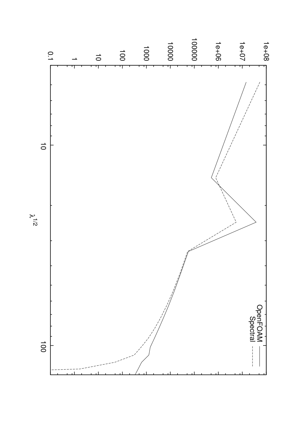
We also compared the power spectral densities for spectral parameter resulting from both codes at ( is the equivalent of the wavenumber in Fourier based spectral decomposition [7]). To this aim we expanded both numerical solutions onto the set of least dissipative modes used in the spectral simulation, following the procedure described in section 3 and compared the kinetic energies corresponding to each value of . The results are presented in fig. 5. Both codes produce quantitatively similar results. Qualitatively, the spectral code seems to be more dissipative, and as a result, more energy is concentrated in the largest scales at the expense of the large-intermediate ones. For mid to small scales up to both codes agree well. The difference in the smallest scales can be explained as follows. The physical space of collocation points is rectangular, so is the spectral domain in the space. Sine curves are a family of cardioids, this space only includes full - shells up to . On these grounds the - PSD spectra is a physically meaningful representation of the solution up to .
4.3 Simulations at high
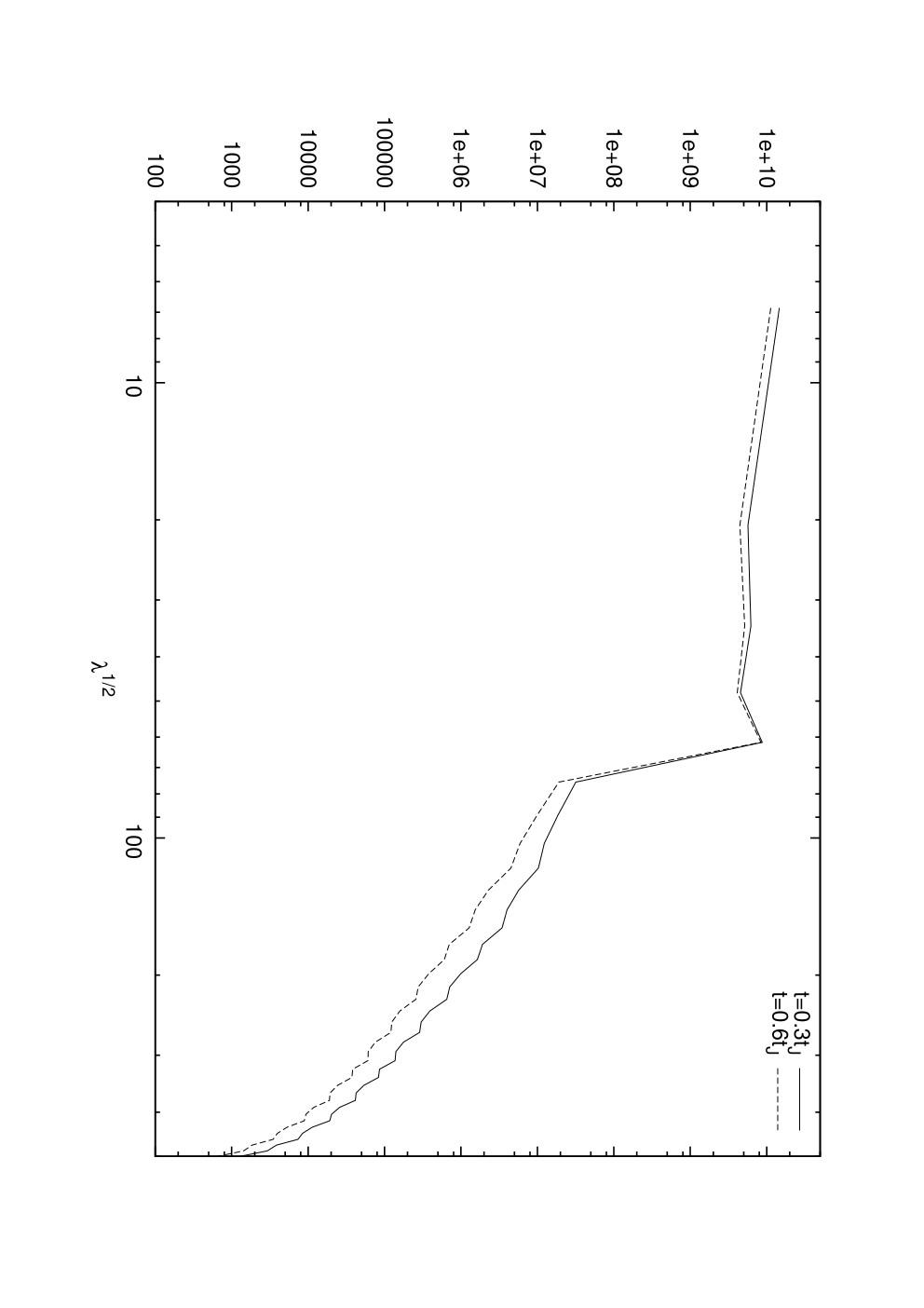
In the previous section we showed that the results obtained with the new spectral approach were able to reproduce the same as those obtained with using finite volume technique, in a case accessible to both methods. For the purpose of this test, we used in our spectral calculations and an effective number of modes (those which were not padded with zeros in the dealiasing procedure), which was the same as the number of grid cells in calculations performed with OpenFOAM. This imposed to choose a rather low Hartmann number so as to keep the computational cost low is both methods. It is, however, for flow at high , that our new approach can potentially offer computational savings, because the theoretically predicted number of degree of freedom is much lower than the number of grid points required in the mesh used in the finite volume method (or in a classical spectral method). The full calculations of decaying or forced MHD turbulence at high are beyond scope of this contribution, as they would require a full scale parallelisation of our code, which is not yet implemented. Our main purpose is to present an implementation of our new spectral method and show that it gives accurate results. Nevertheless, we shall still demonstrate its potential for calculations at higher values of . To this end, we used a different approach to examine the computational savings offered by this new technique. We start with initial conditions determined as in the previous section for . The flow is then evolved for a period of using a spectral basis with a number of modes sufficently high to resolve …so as to erase the trace of the initial non-MHD flow. At this instant we removed from the resulting velocity field all contributions from modes with . The value of was chosen as …the value of the value predicted by [8] for the smallest scales in the forced flow with the forcing on scales and Reynolds number This value is located just behind a sharp drop in PSD, which is an early indication of its relevance as an estimate for the smallest scales. Subsequently we let the flow evolve for another . We then we examined the Power density -spectrum of the resulting velocity field and compared it to that at , seeking in particular if energy had leaked into regions of the spectrum where . The results are presented on fig. 6 We see that the evolution of the spectrum was not significantly influenced. This indicates that the evolution of the flow is sufficiently well described by the modes with , and our method does carry the ability to resolve high flows with the limited number of modes.
5 Computational cost
The cost of pseudospectral codes based on FFT technique scales as . In DNS calculations should be of the order of Reynolds number each. Moreover, to obtain physically meaningful results it is necessary to resolve the Hartmann layer in direction. should therefore be at least of the order of . For large Harmann number calculations the computational cost of FFT based code thus scales as . As explained in sect. 3.3, the spectral decomposition described in sect. 3.2 is only used to treat -dependence while the spectral decomposition in can be performed with FFT. The computational cost in this case scales as . Using the estimation for the number of degrees of freedom in low Rm MHD flows from [16, 3]: , . In sect 3.4, however, we found that it is still necessary to have to calculate accurate spectral coefficients with small errors. Nevertheless, we only need to calculate spectral coefficients, as the rest of them will be dissipated on the very short timescales and are not physically meaningful. Therefore the total computational cost of the proposed scheme scales as . The proposed method has the potential to significantly reduce the computational cost incurred by traditional ones in the regime of high values of , as its computational cost does not depend on the intensity of the magnetic field, which a limiting factor for traditional methods. Theoretically, there is room for additional improvement as the number of degrees of freedom in low Rm MHD flows is inversely proportional to . However, this would require an alternative approach for the treatment of the non-linear terms.
6 Conclusions
We have presented a novel model method to simulate MHD flows in
channel configuration. It is based on using the sequence of least dissipative
eigenmodes from the dissipation operator instead of the traditional Fourier or
Tchebychev basis. The advantage is that these modes show physical properties
of the actual MHD flow. Consequently, the basis requires a smaller number of
modes. On the other hand, they lack the advantageous properties of usual bases,
such as orthogonality and the existence of fast transforms,
which are heavily relied upon in standard spectral methods. We have put forward an approach to
overcome this difficulties and were able to construct a useful numerical
scheme based on this alternative modes. We tested this new method by comparing
its ability to calculate the freely decaying MHD turbulence in a channel to
that of a finite volume code and obtained very good agreement between the two
codes both in terms of global quantities like energy dissipations rates and in
terms of the resulting energy spectra. As a last test, we verified the potential of the
new scheme to efficiently resolve flows in the presence of high magnetic fields
with a limited number of modes.
We would like to stress the large potential of the method we presented.
The scheme we put forward doesn’t depend on any special properties of the used
modes (in particular they don’t have to be orthogonal). Therefore the
procedure can be easily adapted to other MHD and non-MHD problems. The main
idea is to use a basis of functions that already exhibit those features of
the flow, that incur heavy computational cost beyond that
strictly required by the underlying dynamical system (boundary layers typically).
This makes it possible to save the computational time of having to reconstruct
these structures with elements of more standard basis. In favourable cases,
where this operation is computationally expensive (typically when boundary
layers are very thin), this technique has a potential to speed up DNS
calculations by an important factor by restricting the spectral domain to one
more closely embedding that relevant to the calculated flow.
The authors gratefully aknowledge financial support of the Leverhulme Trust (Grant F00/732J). The authors are also grateful to Professor Mahendra Verma, for making the TARANG code available to them and for fruitful discussions around the ideas presented in this paper. Finally the authors would like to express their gratitude to Antoine Huber for his work in the numerical simulations carried out with OpenFOAM.
Appendix A Analytical expression of the eigenmodes of
[7] provides solutions to divergence free eigenvalue problem for operator (6). The eigenvalues are given by dispersion relation:
| (22) |
where for a given can take values and . Therefore they are related by:
| (23) |
A.1 Divergence-free modes
Divergence free eigenvectors can be divided into three subgroups.
A.1.1 Orr-Sommerfeld modes
These are in turn divided based on whether velocity component perpendicular to is symmetric or antisymmetric in .
Symmetric modes:
| (24) | ||||
with and satisfying:
| (25) |
Antisymmetric modes
| (26) | ||||
with and satisfying:
| (27) |
A.1.2 Square modes
Symmetric modes:
| (28) |
with and satisfying:
| (29) |
Antisymmetric modes
| (30) |
with and satisfying:
| (31) |
Quantities and are defined by relations:
A.1.3 Modes with =0
These are the modes in which velocity is function of coordinate only . They are omitted in [7] and we had to derive them independently. Because of the requirement that is divergence free and the non-slip boundary conditions at , has to vanish everywhere. Moreover for this modes. Additionally satisfies boundary conditions imposed on . Therefore in this case the electric potential vanishes in the whole of the domain for the considered modes and the electric current density is given by the expression:
Therefore the eigenvalue problem in this case reduces in dimensionless form to:
Again the modes can be divided into symmetric and antisymmetric ones.
Symmetric modes:
| (32) |
where and q is an odd natural number
Antisymmetric modes:
| (33) |
where and q is an even natural number
A.2 Irrotational modes
Our approach required also derivation of curl-free eigenvectors. They are in one to one relation with Orr-Sommerfeld modes.
Solutions to dispersion relations are such that for a given and every , there are six modes for which .
A.3 Distribution of the modes
For a given and every there are six modes with ,
References
- [1] S. Smolentsev, L. Moreau, R. Buehler, C. Mistrangelo, Mhd thermofluid issues of liquid-metal blankets: Phenomena and advances, Fusion Engineering and Design (2010) 1196–1205.
- [2] T. Boeck, D. Krasnov, E. Zienicke, Numerical study of turbulent magnetohydrodynamic channel flow, J. Fluid Mech. (572) (2007) 179–188.
- [3] A. Pothérat, T. Alboussière, Bounds on the attractor dimension for low-Rm wall-bound MHD turbulence, Phys. Fluids (2006) 25102 (12 pages).
- [4] O. Ladyzhenskaya, The Mathematical theory of viscous imcompressible flow, Gordon and Breach Science Publishers, NY, London, Paris, Montreux, Tokyo, Melbourne, 1968.
- [5] P. W. Livermore, C. A. Jones, S. J. Worland, Spectral radial basis functions for full sphere computations, J. Comp. Phys. (227) (2007) 1209–1224.
- [6] P. H. Roberts, Introduction to Magnetohydrodynamics, Longmans, 1967.
- [7] V. Dymkou, A. Pothérat, Spectral methods based on the least dissipative modes for wall-bounded MHD turbulence, J. Theor. Comp. Fluid Mech. 23 (6) (2009) 535–555.
- [8] A. Pothérat, V. Dymkou, Dns of low-rm mhd turbulence based on the least dissipative modes, J. Fluid Mech. 655 (2010) 174–197.
- [9] M.-J. Ni, R. Munipalli, N. Morley, P. Huang, M. Abdou, A current density conservative scheme for mhd flows at a low magnetic reynolds number. part i. on a rectangular collocated grid system, J. Comp. Phys. 227 (2007) 174–204.
- [10] V. Dousset, A. Pothérat, Characterisation of the flow around a truncated cylinder in a duct in a spanwise magnetic field, J. Fluid Mech. 691 (2012) 341–367.
- [11] C. Canuto, M. Hussaini, A.Quarteroni, T. Zang, Spectral Methods: Fundamentals in Single Domains, Springer-Verlag, 2006.
- [12] M. Frigo, Steven, G. Johnson, The design and implementation of fftw3, in: Proceedings of the IEEE, 2005, pp. 216–231.
- [13] M. K. Verma, A. Chatterjee, S. Reddy, R. Yadav, S. Paul, M. Chandra, R. Samtaney, Benchmarking and scaling stuides of pseudo-spectral code tarang for turbulence simulations, PRAMANA J. Phys. 81 (4) (2013) 617–629.
- [14] R. Klein, A. Pothérat, Appearance of three-dimensionality in wall bouded mhd flows, Phys. Rev. Lett. 104 (3).
- [15] N. Okamoto, P. A. Davidson, Y. Y. Kaneda, On the decay of low-magnetic-reynolds-number turbulence in an imposed magnetic field, J. Fluid Mech. 651 (2010) 295–318.
- [16] A. Pothérat, T. Alboussière, Small scales and anisotropy in low-rm mhd turbulence, Phys. Fluids (2003) 1370–1380.