A density Corrádi–Hajnal TheoremThanks:  * Department of Mathematics, London School of Economics, Houghton Street, London, WC2A 2AE, UK. E-mail: p.d.allen|j.boettcher@lse.ac.ukThanks:  † DIMAP and Mathematics Institute, University of Warwick, Coventry, CV4 7AL, UK. The author is an EPSRC Research Fellow. E-mail: honzahladky@gmail.comThanks: ‡ New Technologies for Information Society, University of West Bohemia, Pilsen, Czech Republic. E-mail: piguet@ntis.zcu.czThanks:  PA, JH, and DP were supported by DIMAP, EPSRC award EP/D063191/1. PA was partially supported by FAPESP (Proc. 2010/09555-7), and JB by FAPESP (Proc. 2009/17831-7). PA and JB are grateful to NUMEC/USP, Núcleo de Modelagem Estocástica e Complexidade of the University of São Paulo, for supporting this research. The research leading to this result has received funding from the European Union’s Seventh Framework Programme (FP7/2007-2013) under grant agreement no. PIEF-GA-2009-253925. An extended abstract of this paper appeared in the proceedings of the Eurocomb 2011 conference. Support by the Institut Mittag-Leffler (Djursholm, Sweden) is gratefully acknowledged.

A classic result of Mantel asserts that each $n$-vertex graph $G$ with more than $\lfloor\frac{n}{2}\rfloor\lceil\frac{n}{2}\rceil$ edges contains a triangle. What can we say about the number of triangles in a graph with more than $\lfloor\frac{n}{2}\rfloor\lceil\frac{n}{2}\rceil$ edges?

There are three natural interpretations of this question. We can ask how many vertex-disjoint triangles are guaranteed, how many edge-disjoint triangles are guaranteed, or simply how many triangles are guaranteed in total. The answer to each of the first two questions is $1$ (which is trivial) and Rademacher proved (see [Erd62a]) that the answer to the last is $\lfloor\tfrac{n}{2}\rfloor$; in each case the extremal example consists of a complete balanced bipartite graph with one edge added to the larger part. It is then natural to ask the same questions of $n$-vertex graphs $G$ with at least $\lfloor\frac{n}{2}\rfloor\lceil\frac{n}{2}\rceil+m$ edges, for any $m\geq 1$.

These questions are much harder. Lovász and Simonovits [LS83] gave a conjectured lower bound on the number of triangles present in any $n$-vertex graph $G$ with at least $\lfloor\frac{n}{2}\rfloor\lceil\frac{n}{2}\rceil+m$ edges, which Erdős [Erd62a] had already proved correct for $m$ small enough compared to $n$. The conjecture remains open, although a celebrated recent result of Razborov [Raz08], using his method of flag algebras, is that the conjectured lower bound—a complicated continuous but only piecewise differentiable function in $m$—is asymptotically correct for all $m$. The number of edge-disjoint triangles was studied by Győri [Győ91], but only for $m\leq 2n-10$ were exact results proved, and for large $m$ it is not clear what the right answer should be.

In this paper we solve (for sufficiently large $n$) the problem of how many vertex-disjoint triangles are guaranteed to exist in an $n$-vertex graph $G$ with a given number of edges. It is convenient to rephrase the problem in the following way.

This problem was first studied by Erdős [Erd62b] and by Moon [Moo68]. The former proved the exact result when $n\geq 400k^{2}$, and the latter when $n\geq 9k/2+4$, giving the following theorem.

Interestingly, although Moon states that his result “almost certainly remains valid for somewhat smaller values of $n$ also”, in fact he almost reaches a natural barrier: the graph which Moon proved to be extremal (the graph $E_{1}(n,k)$ in Definition 5, see also Figure 1) is only extremal when $n\geq 9k/2+3$.

We give an exact solution to Problem 1 for all values of $k$ when $n$ is greater than an absolute constant $n_{0}$. Our main result, Theorem 6, states that the answer is given by four different extremal (families of) graphs in four different regimes of $k$.

We remark that our result can also be seen as a variation of two other classical theorems in extremal graph theory. Firstly, Erdős and Gallai [EG59] answered the analogous question for edges instead of triangles.

In fact, they showed that, depending on $k$, the extremal graph for this problem either consists of $k$ vertices which are complete to all vertices, or of a $(2k+1)$-clique and a disjoint independent set. An analogous behaviour of the extremal structure in the hypergraph case is predicted by the famous Matching Conjecture of Erdős, [Erd65]. In this sense the appearance of various very different extremal structures in our result is not surprising.

Secondly, Corrádi and Hajnal [CH63] considered the variant of Problem 1 where the number of edges is replaced by the minimum degree and proved the following well-known theorem.

The graph $E_{1}(n,k)$ from Definition 5 is also extremal in this setting for the whole range $k\in[0,\frac{n}{3}]$.

Thus, our result is the ‘density version’ of the Corrádi–Hajnal Theorem.

Given an integer $\ell$ and a graph $H$, we write $\ell\times H$ to denote the disjoint union of $\ell$ copies of $H$. We say that a graph is $\ell\times H$-free if it does not contain $\ell$ vertex disjoint (not necessarily induced) copies of $H$. In Theorem 6 we determine the maximal number of edges in a $(k+1)\times K_{3}$-free graph on $n$ vertices for every $0\leq k<\frac{n}{3}$. The extremal formula is a somewhat opaque maximum of four different terms, so in preference to presenting it we shall describe four constructions of $n$-vertex $(k+1)\times K_{3}$-free graphs corresponding to these four terms. We say that an edge $e$ (or more generally a set of vertices) meets a set of vertices $X$ if $e$ and $X$ intersect. The edge $e$ meets $X$ in $X^{\prime}$ if $X^{\prime}=X\cap e$.

Our main result is the following.

For three sets $A,B,C$ (not necessarily distinct) we say that a triangle $uvw$ is of type $ABC$, if $u\in A,v\in B$, and $w\in C$. All triangles in $E_{1}(n,k)$ are of type $XY_{1}Y_{2}$, $XXY_{i},i=1,2$, or $XXX$, thus intersecting $X$ at least once. Thus $E_{1}(n,k)$ contains at most $k$ vertex-disjoint triangles. All triangles in $E_{2}(n,k)$ and in $E_{3}(n,k)$ are of type $XXY_{1}$, or $XXX$, intersecting $X$ at least twice. Therefore these two graphs do not contain more than $k$ vertex-disjoint triangles. All triangles in $E_{4}(n,k)$ must be fully contained in $X\cup Y_{1}\cup Y_{2}$ and therefore there are at most $\lfloor\frac{1}{3}|X\cup Y_{1}\cup Y_{2}|\rfloor=k$ vertex-disjoint triangles.

The graphs $E_{i}(n,k)$ are edge-maximal subject to not containing $(k+1)\times K_{3}$. The only exception is $E_{4}(n,k)$ for $k\lesssim\frac{n}{4}$. Indeed, when $k<\frac{n}{4}-1$, we have $|X|<2k$. Therefore, in any collection of $k$ vertex-disjoint triangles, there must be at least $w=2k-|X|$ triangles of type $XY_{1}Y_{2}$. Thus, if $|Y_{1}|\leq w$, one can actually add edges inside $Y_{1}$ without increasing the maximum number of vertex-disjoint triangles. However $E_{4}(n,k)$ is in any case not the extremal graph in this range; see the discussion below and Table 1. The graphs $E_{i}(n,k)$ have the following numbers of edges (after an exact formula we identify the leading terms; to this end we use the symbol $\approx$).

Comparing these edge numbers reveals that, as $k$ grows from $0$ to $n/3$, the extremal graphs dominate in the following order (for $n$ sufficiently large). In the beginning $E_{1}(n,k)$ has the most edges of these four graphs until $k\approx\frac{2n}{9}$, where it is surpassed by $E_{2}(n,k)$. At $k\approx\frac{n}{4}$ this extremal structure ceases to exist and is replaced by $E_{3}(n,k)$, until finally at $k\approx(5+\sqrt{3})n/22$ the graph $E_{4}(n,k)$ takes over. The exact thresholds are listed in Table 1. Further, the edge numbers of the graphs $E_{i}(n,k)$ are plotted in Figure 2.

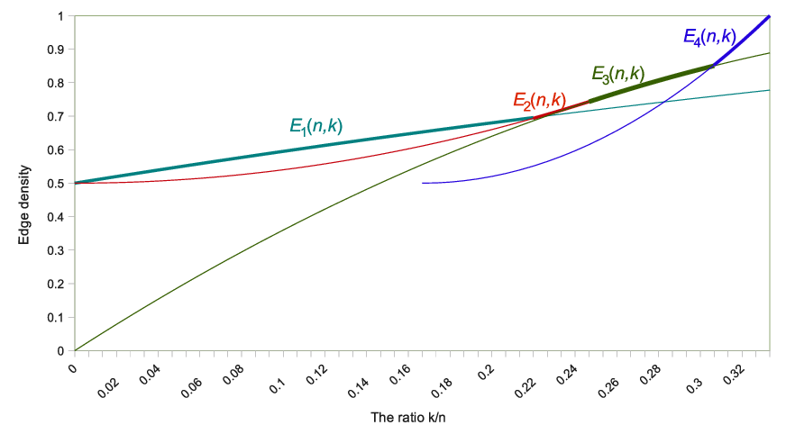
Observe that for fixed $n$, as $k$ increases, the transitions of the extremal graphs from $E_{1}(n,k)$ to $E_{2}(n,k)$ and from $E_{3}(n,k)$ to $E_{4}(n,k)$ are not continuous: $\Theta(n^{2})$ edges must be edited to change from the former to the latter structure. The transition from $E_{2}(n,k)$ to $E_{3}(n,k)$ however is continuous.

The basic idea of our proof is straightforward: we show that we can partition the vertices of any $(k+1)\times K_{3}$-free graph into six parts, and establish some upper bounds on the numbers of edges within and between these parts in terms of their sizes only. This defines a function (of six variables) which is an upper bound on the number of edges of a graph with parts of the given sizes. Then maximising this function (subject to $n$ and $k$ being fixed) we obtain an upper bound on the number of edges of a $(k+1)\times K_{3}$-free graph with $n$ vertices, and observe that this matches the lower bounds provided by the extremal structures given in Definition 5.

We shall now fix the basic setup for our proof, i.e., we will specify the above mentioned six parts, which will be called $\mathcal{T}_{1}$, $\mathcal{T}_{2}$, $\mathcal{T}_{3}$, $\mathcal{T}_{4}$, $\mathcal{M}$, and $\mathcal{I}$. We need the following definition. Let $G$ be a graph, $uv$ be an edge in $G$ and $xyz$ a triangle in $G$. We say that $uv$ sees vertex $x$ of $xyz$ if $uvx$ is a triangle in $G$. The edge $uv$ sees $xyz$ if $uv$ sees at least one of the vertices $x$, $y$, or $z$. Similarly, we say that a vertex $u$ sees (the edge $xy$ of) the triangle $xyz$ if $uxy$ is a triangle in $G$.

Throughout we will assume the following setup.

We remark that the outcome of the algorithm for constructing $\mathcal{T}_{3}$ and $\mathcal{T}_{4}$ is not uniquely determined. However, any possible pair $\mathcal{T}_{3}$ and $\mathcal{T}_{4}$ resulting from the construction we described is suitable for our purposes.

Further, we emphasise that $k=|\mathcal{T}|$ is the number of triangles in $\mathcal{T}$, which cover $3k$ vertices (and similarly $\mathcal{M}$ covers $2m$ vertices). The function $e(\bullet)$ counts the number of edges in $G$ induced by the structure $\bullet$, e.g., $e(\mathcal{T}_{3})=e(G[V(\mathcal{T}_{3})])$. Similarly, $e(\bullet,\star)$ counts edges in the bipartite graph between the structures $\bullet$ and $\star$.

Before we proceed, let us give some motivation for the above defined partition of $G$ by applying it to our four extremal graphs from Definition 5. First consider the graph $E_{1}(n,k)$. It is easy to check that for this graph we have $\mathcal{T}=\mathcal{T}_{1}$ in the range when this graph is optimal (see Table 1), and all vertices (except perhaps one) outside $\mathcal{T}$ are in $\mathcal{M}$. Any pair of triangles of $\mathcal{T}$ has seven edges between them in $E_{1}(n,k)$, the set $\mathcal{M}$ induces $m^{2}$ edges, and $e(\mathcal{M},\mathcal{T}_{1})=4mt_{1}$. We shall show in our proof that in any graph $G$, the definition of $\mathcal{T}_{1}$ forces that any two triangles of $\mathcal{T}_{1}$ have at most seven edges between them (see Lemma 10( ) ‣ 10), the set $\mathcal{M}$ induces at most $m^{2}$ edges (see Lemma 10( ) ‣ 10), and $e(\mathcal{M},\mathcal{T}_{1})\leq 4mt_{1}$ (see Lemma 10( ) ‣ 10). Together with bounds which we will prove on the number of edges touching $\mathcal{I}$, we conclude that if $\mathcal{T}=\mathcal{T}_{1}$ then $e(G)\leq e\big(E_{1}(n,k)\big)$.

Similarly, the definition of $\mathcal{T}_{2}$ and $\mathcal{T}_{4}$ is motivated by the fact that in both $E_{2}(n,k)$ and $E_{3}(n,k)$ we have $\mathcal{T}=\mathcal{T}_{2}$, while in $E_{4}(n,k)$ we have $\mathcal{T}=\mathcal{T}_{4}$ (again in the appropriate range). The set $\mathcal{T}_{3}$ is always empty in the extremal graphs. It turns out that, for $E_{2}(n,k)$ and $E_{3}(n,k)$ we will be able to use a similar strategy as lined out for $E_{1}(n,k)$, i.e., we shall infer from the definition of $\mathcal{T}_{2}$ that $E_{2}(n,k)$ and $E_{3}(n,k)$ have a maximal number of edges in $\mathcal{T}_{2}$ (see Lemma 10( ) ‣ 10) and then show that $\mathcal{T}=\mathcal{T}_{2}$ in an extremal graph (for the appropriate range of $k$). For $E_{4}(n,k)$ we must work harder: the definition of $\mathcal{T}_{4}$ permits nine edges to exist between a pair of triangles, yet in $E_{4}(n,k)$ only some pairs of triangles actually have nine edges between them (see Table 2).

As explained, our main goal in the following will be to establish bounds on the number of edges within and between the six parts of $G$. One concept that will turn out to be very fruitful in this context is that of a rotation.

Typically, the rotations that we will consider are local structures. To give an example, let $G$ and $\mathcal{T}$ be as in Setup 7. By definition, there are no improving rotations in $G$. Suppose, however, that we find outside $\mathcal{T}$ two vertex-disjoint edges $uv$ and $u^{\prime}v^{\prime}$, and a triangle $xyz$ of $\mathcal{T}$ with the property that $x$ is a common neighbour of $uv$, and $y$ of $u^{\prime}v^{\prime}$. This structure allows us to rotate by replacing $xyz$ with $uvx$ and $u^{\prime}v^{\prime}y$, a contradiction. The non-existence of this structure leads to an upper bound on the number of edges between $\mathcal{M}$ and $\mathcal{T}$.

In this section we will describe several rotations involving small numbers (one or two) of triangles, and show that their non-existence gives good bounds on the maximum number of edges within and between $\mathcal{T}_{1}$, $\mathcal{T}_{2}$, $\mathcal{T}_{3}$, $\mathcal{M}$ and $\mathcal{I}$. The bounds obtained on edges involving $\mathcal{T}_{4}$ are not strong enough for the proof of Theorem 6, but they are strong enough to prove the following lemma, which serves both as an illustration of our technique and as a necessary step in the proof of Theorem 6.

Observe that, in contrast to Theorem 6 we do not require any lower bound on $n$ in this lemma. Observe also that since $\tfrac{n-8}{5}<\tfrac{2n-8}{9}$, the result follows from Theorem 2: but its proof will exemplify our techniques and put us into position to explain the remaining steps to obtain Theorem 6.

We assume in the following Setup 7. We start with some simple upper bounds.

We next come to two bounds on edges within $\mathcal{T}$.

Our next task is to bound the edges between $\mathcal{M}$ and $\mathcal{T}_{j}$, $j\geq 2$, and between $\mathcal{I}$ and $\mathcal{T}_{j}$, $j\geq 3$. We combine these bounds with those given in Lemma 11 because they permit us to handle the cases $t_{1}=1$ and $t_{2}=1$ which were not dealt with in Lemma 11. However, in the proof of Theorem 6 we will find that we require both sets of bounds.

References

- [ABHP] P. Allen, J. Böttcher, J. Hladký, and D. Piguet. An extension of Turán’s Theorem, uniqueness, and stability. arXiv:1403.3801.
- [ABHP13] P. Allen, J. Böttcher, J. Hladký, and D. Piguet. Turánnical hypergraphs. Random Structures Algorithms, 42(1):29–58, 2013.
- [CH63] K. Corrádi and A. Hajnal. On the maximal number of independent circuits in a graph. Acta Math. Acad. Sci. Hungar., 14:423–439, 1963.
- [EG59] P. Erdős and T. Gallai. On maximal paths and circuits of graphs. Acta Math. Acad. Sci. Hungar, 10:337–356 (unbound insert), 1959.
- [Erd62a] P. Erdős. On a theorem of Rademacher-Turán. Illinois Journal of Mathematics, 6:122–127, 1962.
- [Erd62b] P. Erdős. Über ein Extremalproblem in der Graphentheorie. Arch. Math., 13:222–227, 1962.
- [Erd65] P. Erdős. A problem on independent -tuples. Ann. Univ. Sci. Budapest. Eötvös Sect. Math., 8:93–95, 1965.
- [Erd68] P. Erdős. On some new inequalities concerning extremal properties of graphs. In Theory of Graphs (Proc. Colloq., Tihany, 1966), pages 77–81. Academic Press, New York, 1968.
- [GH12] C. Grosu and J. Hladký. The extremal function for partial bipartite tilings. European J. Combin., 33(5):807–815, 2012.
- [Győ91] E. Győri. On the number of edge disjoint cliques in graphs of given size. Combinatorica, 11(3):231–243, 1991.
- [HS70] A. Hajnal and E. Szemerédi. Proof of a conjecture of P. Erdős. In Combinatorial theory and its applications, II (Proc. Colloq., Balatonfüred, 1969), pages 601–623. North-Holland, Amsterdam, 1970.
- [Kom00] J. Komlós. Tiling Turán theorems. Combinatorica, 20(2):203–218, 2000.
- [LS83] L. Lovász and M. Simonovits. On the number of complete subgraphs of a graph. II. In Studies in pure mathematics, pages 459–495. Birkhäuser, Basel, 1983.
- [Moo68] J. W. Moon. On independent complete subgraphs in a graph. Canad. J. Math., 20:95–102, 1968.
- [Raz08] A. A. Razborov. On the minimal density of triangles in graphs. Combin. Probab. Comput., 17(4):603–618, 2008.
- [Sim68] M. Simonovits. A method for solving extremal problems in graph theory, stability problems. In Theory of Graphs (Proc. Colloq., Tihany, 1966), pages 279–319. Academic Press, New York, 1968.
Appendix A Maximisations
In this section we provide proofs of Lemmas 13, 19, and 20. These lemmas concern maximisations of certain functions. We build our arguments on tedious elementary algebraic manipulations. While some of the statements we need could be obtained by a more routine technique of Lagrange multipliers, this method seems to lead to even lengthier calculations in our setting. This is caused in particular by a high degree of discontinuity, caused by various case distinctions and appearance of the floor/ceiling function, of the functions we want to maximise.
We first collect some useful statements relating to , all of which are obtained by simple calculation using equations (3) and (4). The three relations (22)–(24) below hold for any .