Phase diagram study of a dimerized spin-S zig-zag ladder

If $\forall_{i}$ $0<J(i),J^{\prime}(i),J_{2}(i),J^{{}^{\prime}}_{2}(i)$, the system becomes frustrated, which in general implies a complex structure of the GS and its excitation. In this case some of the usual techniques used to deal with this kind of problems may fail at zero temperature. However, for $J^{\prime}(i)=J_{2}(i)+J_{2}^{{}^{\prime}}(i)<J(i)$, the Hamiltonian (1) presents a factorized eigenstate which corresponds to the GS for $J^{\prime}S\ll\min_{i}J(i)$. To see it, we can rewrite the Hamiltonian in terms of local operators on each rung:

where

$\vec{\bf J}_{i}$ is the total angular momentum of the rung $i$, and $\vec{\bf K}_{i}$ is another set of local vectorial observable which completes the full local Lie algebra relevant to the problem. Its components close the following Lie algebra:

where $\epsilon_{\mu\nu\eta}$ is the fully antisymmetric Levi-Civita symbol and ${\bf i}=\sqrt{-1}$ is the imaginary unit. If we set the constraints

the last term in (2) vanishes and the state

results an eigenstate of ${\bf H}$ with energy $E_{\rm dim}=-JNS(S+1)$, due to $\vec{\bf J}_{i}|{\rm singlet}\rangle_{i}=0$. Noteworthy, this result is valid for any value of the local spin magnitude $S$.

The state (7) has not a classical analog in terms of individual classical magnetic moments, corresponding to a phase with a characteristic quantum behavior: a dimerized phase. In this phase, despite the spin-spin correlations vanish between non continuous sites, there could exist correlations between pairs of its elementary excitations. Another characteristic of this order is that there is a spin gap which prevents the occurrence of a spontaneous breaking in the global $SU(2)$ symmetry. However, the determination of the gap can be a non-simple task. Although the dimerized GS may remains stable when we change the couplings maintaining the constraint (6), the excited states strongly depend on the values of the local couplings.

The few systems where an exact GS can be obtained have played a very important role in quantum magnetism. For example, we can cite the exact GS of the AKLT point [1] which has been very important in the confirmation of Haldane’s prediction [2] that the spectrum of an integer-S spin chains is gaped. In the present model, the dimerized eigenstate is surprisingly robust. For example we can change the couplings $J(i)$, $J^{\prime}(i)$ and $J_{2}(i)$ in Hamiltonian (1) and, preserving the constraints (6), the dimerized state is still an eigenstate; this is a very important property inside the regions where this eigenstate is the GS of the system: since excited states are strongly dependent of the distribution of couplings, we can change the distribution of couplings in order to reduce the gap. A similar property of the AKLT model can be exploited for spin 1. In fact a very interesting question is if it there exists some coupling distribution that makes the system gapless. The advantage of this system is that its robust GS is present over a extended region of the very large parameter space for any value of the local spin. Since the excited states in the general case can be very complicated, a such study of the many possible excited states deserves a separate publication. In order to obtain a qualitative picture, in the present manuscript we focus mainly on the restricted case of the uniform ladder $J(i)=J$, $J^{\prime}(i)=J^{\prime}$ and $J_{2}(i)=J^{\prime}_{2}(i)=J_{2}$, where $J$, $J^{\prime}$ and $J_{2}$ are positive and site-independent numbers. Besides, to avoid boundary effects, we will restrict to the case of periodic boundary conditions and $N$ even. Under these assumptions, we can easily show that the $|{\rm dimer}\rangle$ state in Equation (8) is a true GS of the system if the condition

is provided. To see this, we can write the Hamiltonian (1) in a more convenient way:

with

where $\delta J=J-J^{\prime}$. From this decomposition we can see that the GS energy per rung is

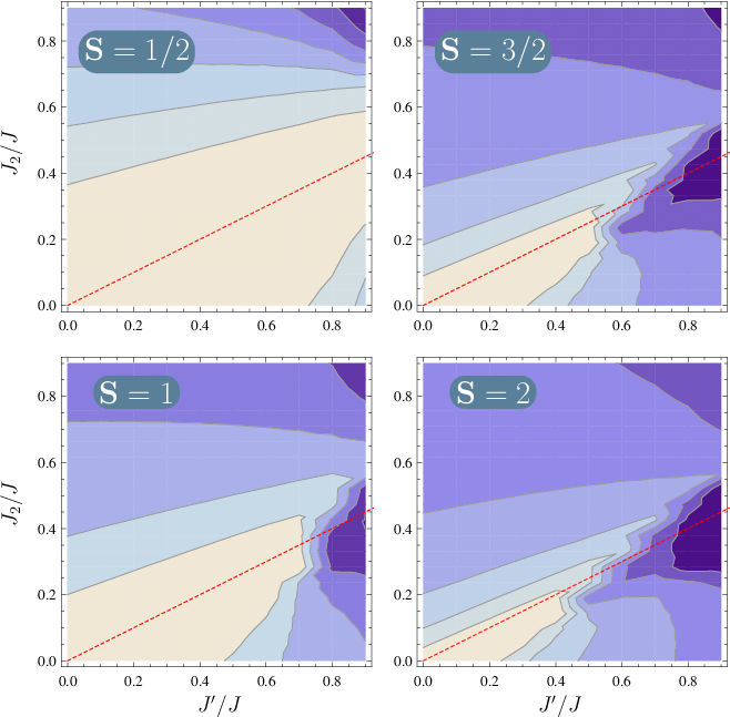
where the right hand side corresponds to the minimum eigenvalue of all the ${\bf h}_{i}$ terms. When the condition (9) is satisfied, this lower bound coincides with the energy associated to the state $|{\rm dimer}\rangle$ and hence, it is a GS. Moreover, due to for $J>J^{\prime}$ there is not any other state which minimizes all the ${\bf h}_{i}$ at a time and hence, this GS results non-degenerated. Equation (9) represents a sufficient condition for the existence of the dimerized GS, but the true range of couplings where this state is a real GS can be larger. In Figure 2 the relative energy $E_{\rm GS}/E_{\rm dim}-1$ as a function of $J^{\prime}/J$ over the line $J_{2}=\frac{J^{\prime}}{2}$ for a $2\,N=40$ sites system with different local spin values is depicted. This quantity vanishes when the energy of the system is equal to the energy of the dimerized eigenstate. We can see that for a given spin $S$, the values of $J^{\prime}$ where $E_{\rm GS}/E_{\rm dim}-1$ becomes different from zero are larger than the values predicted in Eq. (9). Dashed line corresponds to the single site mean field result discussed in the next Section, corresponding to the large $S$ limit. In Section 4 we show that for large $S$ the next to leading order is proportional to $S^{-1}$. In the next section we will show also that if $J^{\prime}/J>\sqrt{2/S}$ there is a fully factorized state (the mean field state) which has energy lower than the dimerized eigenstate. This allow us to obtain an upper bound value for the transition coupling $J_{c}(S)$, whereas Eq. (9) represents a lower bound.

In Figure 3 we show the relative energy calculated by DMRG as a function of $J_{2}$ for different values of $S$. Upper panel corresponds to $J^{\prime}=0.6$ where the systems with $S=1/2$ and $S=1$ reach the fully-dimerized GS at the $J_{2}=J^{\prime}/2=0.3J$ point. We can observe in the figure that, for this two cases, the curves come together at that point, whereas the curves corresponding to $S=3/2$ and $S=2$ have a lower energy (which corresponds to a larger relative energy). Lower panel in Fig. 3 corresponds to $J^{\prime}=0.8$ where just the $S=1/2$ system reaches the dimerized GS.

The GS of the “classical” model can be known by studying a unit cell, as composed by two magnetic moments with fixed magnitude. This approach is equivalent to look for an variational approximation over the family of product states of fully polarized spin states

Besides, because the Hamiltonian that we are considering is linear on each local spin projection operators, this approach is completely equivalent to a full mean field treatment. In this way, the problem is reduced to find the angles determining the directions of all local spins, which can be found by numerical methods, for instance, in a self-consistent way. To allow us to go forward in an analytical description, we can reduce the problem by looking for solutions over a subfamily with certain symmetries. A first reasonable assumption is that the states that we are looking for are symmetrical under a reflection with respect to the plane $xz$, which is a symmetry of the Hamiltonian. For this reason, we can expect that there were a solution with all the states $|\vec{s}_{i}\rangle$ polarized in that plane¹¹ 1 For finite systems, a numerical analysis shows that in general, the energy can be lowered if we allow the magnetic moments to move sightly away from the plane.. A second assumption is that $\forall_{i}$ the angle between $\vec{s}_{k}$ and $\vec{s}_{k+2}$ is constant, due to the global translational symmetry. The resulting family corresponds to the planar spiral states

being $|\varphi\rangle=\exp(-{\bf i}\varphi{\bf S}^{y})|\rightarrow\rangle$ the local coherent state polarized along the direction $\vec{s}=(\cos(\varphi),0,\sin(\varphi))$. The energy $E_{\rm sep}[\theta,\phi]=\langle\theta\phi|{\bf H}|\theta\phi\rangle$ is hence given by

Looking for the extremes of this function we obtain the following energies

where

Phases corresponding to energies $E_{\rm sep}(\pi,\pi)$ and $E_{\rm sep}(0,\pi)$ are labeled as $(\pi,\pi)$ and $(0,\pi)$ respectively, and corresponds to two different Néel orders. The phase with energy $E_{\rm sep}(\tilde{\theta},\tilde{\phi})$ is a spiral phase (see Fig. 4 ).

If we consider now the case of $J^{\prime}=2J_{2}$, $\cos(\tilde{\theta})\rightarrow-\frac{J^{\prime}}{2J}$, $\tilde{\phi}\rightarrow 2(\pi-\tilde{\theta})$ and the energy results

We can make two observations about it. On the one hand, we can see that for $(J^{\prime}/J)^{2}>\frac{2}{S}$ the energy of this mean field is lower than the associated to the dimerized state, which suggests to identify the “classical limit” with the “large $S$ limit”. On the other hand, for small spin, we can observe that this state is a very rough approximation to the true GS in several ways: First of all, for $S\leq 1$, $\frac{E_{\rm sep}-E_{\rm GS}}{E_{\rm GS}}\approx 1$, in a way that does not allow us to consider the difference as an small correction over the mean field result. Other symptom of the in-accurateness of the approximation is related to the lack of similarity between the true GS and the optimum spiral state. In order to quantify this difference, we can compute the Fidelity [28] between the density matrix of any pair of spins. The fidelity is defined as

(see B) where $\rho_{1,2}$ are two different density matrices. For pure states ($\rho_{i}=|\psi_{i}\rangle\langle\psi_{i}|$), this quantity is reduced to the absolute value of the overlap between both states ${\cal F}[|\psi_{1}\rangle|\psi_{2}\rangle]=|\langle\psi_{1}|\psi_{2}\rangle|$. In the dimer state, the density matrix of any pair of spins is given by

while for the spiral state

which leads to the fidelities

These low values of fidelity indicate a very poor accuracy in the estimation of some mean values provided by MFA. A typical way to improve these results consists in implementing a symmetry restoration over the mean field results²² 2 Here we assume that the true GS is non-degenerate, and hence, is $SU(2)$ invariant, belonging to the $j_{T}=0$ sector.:

where $d\mu_{\Omega}$ is the normalized invariant measure of $SU(2)$ and ${\bf R}_{\Omega}$ is a given global rotation. The state $|\rm{SR\,MF}\rangle$ is then the projection of the $|\rm MF\rangle$ over an eigenspace of the total angular momentum operator ${\bf J}_{t}^{2}$, built as a coherent superposition of all other states obtained by global rotations[29]. In finite size systems ($N,S<\infty$) a suitable choice of the representation of ${\rm R}_{\Omega}$ leads to reduce the energy associated to $|\rm{SR\,MF}\rangle$ slightly below the mean field result.

The local state of a given subsystem ${\cal A}$ is obtained as the partial trace over the complementary subsystem $\bar{\cal A}$:

Notice that the integrand in (20b) is not hermitian, but the integral is it. For large $S$ or $n_{\bar{\cal A}}$, $w_{\cal A}[\Omega,\Omega^{\prime}]\rightarrow\delta(\Omega-\Omega^{\prime})$ (see C) and hence³³ 3 This result also corresponds to average the reduced state over all possible mean field solutions. It can also be derived through a path integral approach as the Static Path Approximation[30].

Due that the energy depends on the pairs local states, it implies that the symmetrized state in the large $N$ limit has the same energy than the spiral one.

Exploiting the structure of the state, we can rewrite the local statistical operator as $\rho^{\rm SR}_{\cal A}=\sum_{j}p^{\cal A}_{j}\Pi^{\cal A}_{j}$ where $\Pi^{\cal A}_{j}$ is the projector over the total spin in ${\cal A}$ and $p_{j}^{\cal A}=\langle{\rm spiral}|\Pi_{j}^{\cal A}|{\rm spiral}\rangle$.

In order to check the accuracy of the approximation, we will consider the state of the subsystem defined by a pair of spins inside a same rung $\rho_{\rm rung}$. In the top panels of Figure 5, ${\cal F}[\rho_{\rm rung}^{ex},\rho_{\rm rung}^{\rm SRMF}]$ is depicted for different $S=1/2,1,3/2$ and $2$, over the line $J^{\prime}=2J_{2}$, as a function of $J^{\prime}$ (left) and over the line $J^{\prime}=0.6J$ as a function of $J_{2}$ (right)⁴⁴ 4 In this case, the reference values for the local density matrices were obtained by means of the Lanczos method for numerical exact diagonalization (see A).. On the bottom panels, the corresponding fidelities to the local singlet state are depicted. On the one hand, we observe that over the dimerizing line $J^{\prime}=J_{2}/2$ the fidelity between the exact and the SRMF state is reduced as the spin grows up, and is sightly decreasing, up to the point in which the $|{\rm dimer}\rangle$ ceases to be the GS. At this point, the fidelity gives a jump, and start to increase with $J^{\prime}$. On the other hand, we observe that if we move crossing the dimerizing line with constant $J^{\prime}/J$, the fidelity with respect on the SRMF local state has a minimum in those cases for which the system reach dimerization (for the $J^{\prime}=0.6J$ case, $S=1/2,1$), whereas when the dimerization is not reached, (for $J^{\prime}=0.6J$, $S=3/2,2$) the behavior is the opposite. At the same time, the fidelity with the singlet state falls of up to a value of $0.5$, and continues decreasing with $J^{\prime}$.

As we say before, the “classical” mean field is not suitable to represent the system in a dimerized phase. In particular, for $S=1/2$, we know that the exact solution corresponds to such a phase for $2J_{2}-J^{\prime}=0$ and $J^{\prime}<J$. In this way, a better starting point to improve the mean field approximation is to choose as the unit cell those pairs of spins coupled by the stronger interaction. For instance, if $J>J_{2},J^{\prime}$, we will look for mean field solutions of the form

where $|\alpha_{i}\rangle\in{\mathcal{H}}_{2\,i-1}\otimes{\mathcal{H}}_{2\,i}$. In order to simplify the further discussion, we introduce the parameter $\gamma=\frac{2J_{2}-J}{J}\frac{S(S+1)}{3/4}$ which, together with $J^{\prime}$, determines each point in the phase diagram. For $\gamma=0$, the lowest energy mean field state is obtained for $|\alpha_{i}\rangle=|{\rm singlet}\rangle$, and coincides with the “exact” GS (7). For small enough $|\gamma|$ we can expect that the true ground state results similar to the dimer state. To drive the mean field optimization problem to a simpler form, we will restrict a little bit the family, but in a way that it still contains both the spiral ordered “classical” state as well the dimerized state. This can be achieved by setting $|\alpha_{i}\rangle=({\bf R}(\theta))^{i}|\alpha_{1}\rangle$ with ${\bf R}(\theta)$ a fixed planar rotation. Also, due to the global rotational symmetry, we can choose $|\alpha_{1}\rangle$ as an state with total spin $\langle\vec{\bf J}\rangle$ polarized in the $x$ direction, and both local spin mean values laying on the $xz$ plane. With these assumptions, we can face in a analytical way the mean field problem for the $S=1/2$ case: in such a case, we have to consider a one-parameter family:

where $|\mu\rangle$ ($\mu=x,y,z$) are the states such that ${\bf J}^{2}|\mu\rangle=2|\mu\rangle$ and ${\bf J}_{\mu}|\mu\rangle=0$, and $\zeta$, $\phi$, $\tau$ and $\theta$ are parameters ranging on $0\leq\zeta<\frac{\pi}{2}$, $0\leq\phi<\pi$, $-\pi/2\leq\tau\leq\pi/2$,$-\pi<\theta<\pi$.

It is easy to verify that $\tau$ does not modifies the internal energy of the pair, but just the magnitude of the local spin mean values. For this reason, the optimum state always belongs to the subset $\tau=0$. The remaining parameters have a direct interpretation: the local mean field spin values have equal magnitudes $|\langle\vec{\bf S}_{i}\rangle|=\frac{\sin(\zeta)}{2}$, being $\phi$ the angle between them. With this parametrization, the separable case in Eq. (11) is obtained for $\zeta=\pi/2$ whereas for $\zeta=0$ the $|{\rm singlet}\rangle$ is recovered. For the general case, the variational energy is given by

For $\zeta=\pi/2$, the previous expression is reduced to (13), corresponding to a factorized state, but is easy to check that the minima of (13) does not correspond to global minimum for (23). For $|\gamma|<1$, the true minimum is attained for $\zeta=0$, $\phi=\pi$, corresponding to the dimerized state (7), with energy $E_{{\rm MF_{pair}}}[\theta,\zeta,\phi]=E_{dimer}=-\frac{3}{4}JN$, which means that we can expect a dimerized phase in all this region.

On the other hand, for $|\gamma|>1$, but keeping $|J^{\prime}|<J$ the minimum is attained for $\phi=\pi$, $\cos(\theta)=\frac{-\gamma}{|\gamma|}$ and $\cos(\zeta)=\frac{1}{|\gamma|}$, with energy $E_{{\rm MF_{pair}}}[\theta,\zeta,\phi]=-\frac{1}{4}JN(\frac{1}{|\gamma|}+1+|\gamma|)$. This phase is characterized by a breaking of the $SU(2)$ symmetry but, differently to the large $S$ prediction, this phase results colinear instead of spiral. Another difference is related with the degree of symmetry breakdown: for $|\gamma|\gtrsim 1$, the difference between the the local states associated to the corresponding mean field state and such obtained by the symmetry projection method discussed before are not very important. On the other hand, as $|\gamma|$ grows, the mean field becomes near to the single site mean field result, for which the symmetry projection is required.

For $S>1/2$, the fully analytical treatment discussed in the previous paragraph is not feasible anymore, because the local basis grows as $S^{2}$. For small $S$ we can try to solve the full mean field equation numerically by a self-consistent treatment or any other high dimension optimization method. However, in order to look for analytical solutions, we can search it in a reasonable reduced family. Probably, a good starting point is given by the family of states generated by the singlet state and a general fully factorized spiral state (12). Up to a global rotation, the most general local state in this family is given by

with ${\cal N}^{-1}=\sqrt{1-\frac{\sin(\zeta)\cos(\tau)\sin^{2S}(\phi/2)}{\sqrt{2S+1}}}$. Indeed, the solution for the pair mean field in the $S=1/2$ case always belongs to this family. The energy associated to this family of states is given by

being $E_{\rm ESP}[\theta,\phi]$ the energy associated to the fully separable spiral state defined in (13). For $S\leq 3/2$, over the line $J^{\prime}=2J_{2}$ the energy is always optimized for the fully-dimerized state, while for $S\geq 2$, the optimum value is attained at the fully factorized classical state for $J^{\prime}>J^{\prime}_{c}=2J/S$, what can be see as a first order phase transition. This result could sound disappointing: a direct mean field treatment, even if we consider the complex cell proposed here, is not able to reproduce the transition between the dimerized and the spiral phases. However, examining the behavior of the fidelities between the exact state and the single site mean field + symmetry restoration (see Fig 5), we observe that at least locally, after the transition the local state of the strong correlated pairs tends to the mean field result, including the cases for which the pair mean field solution predicts dimerization. In this way, we can not expect to obtain a better mean field solution by exploring a larger family, leading to understand it as a genuine collective full quantum effect, coming from the quantum corrections to the correlation energy on the excited states. This point will be discussed more detailedly in the next section.

If we start from a single site mean field, RPA scheme (26) always leads to the local approximate bosonization

where $\mathbf{S}^{\mu^{\prime}}_{i}$ are the components of local spin operator in an intrinsic basis $(x^{\prime},y,z^{\prime})$ chosen in a way that the local spin polarization points in the $z^{\prime}$ direction. This bosonization leads to a spin wave-like Hamiltonian

with ${\bf z}={{\bf b}_{1},\ldots{\bf b}_{2N}}$ a “vector” of bosonic operators, $\Lambda={\rm diag}(\varepsilon_{i}^{(\rm MF)})$ a diagonal matrix with elements equal to the local mean field Hamiltonian excitation energies, and ${\cal H}$ a matrix with the block form

For the translational invariant coplanar mean field case (Eq. 12), we can diagonalize the quadratic form analytically: starting with the Fourier transform,

we can rewrite the Hamiltonian as

where

and

with $\Delta_{k}^{\pm}$ blocks defined by

Now, by means a canonical transformation we diagonalize each ${\cal H}_{k}$. We can recover the excitation energies in terms of invariants of the ${\cal H}_{k}$ matrices:

Zero modes arise when $\det{\cal H}_{k}=0$. This happens always for $k=0$ and $k=\tilde{\theta}$, corresponding to Goldstone modes associated global rotations around the global $y$ axes or an axes over the global $xy$ plane respectively.

Around the line $\gamma=0$, we know that for $S=1/2$ the mean field state is always the dimerized state (7), and that, for small enough $J^{\prime}$, there is always a region for which this result holds for any spin $S$. To obtain the RPA Hamiltonian associated to this mean field solution is useful to start from the expression (2). Due to the structure of the Hamiltonian, the relevant local basis for this problem is given by $(|{\rm singlet}\rangle,|x\rangle,|y\rangle,|z\rangle)$ where $|\mu\rangle=\sqrt{\frac{3/4}{S(S+1)}}{\bf K}_{\mu}|{\rm singlet}\rangle$. Using the algebraic properties of the ${\bf K}_{\mu}$ operators defined in (4) we can check that this is an orthonormalized basis. Following the RPA prescription (Eq. (26)) we obtain the approximate bosonic map:

It leads to the bosonized Hamiltonian

with

This is, in this approximation the system is mapped to three decoupled bosonic systems with first neighbor quadratic interactions. For $\gamma=0$, the systems become decoupled, due to the fact that the mean field state corresponds to a true GS. For general $\gamma$, the excitation energies of any of ${\bf h}_{\mu}^{\rm bos}$ are given by

The correction to the ground state energy is hence given by

where ${\rm E}(x)=\int_{0}^{\pi/2}\sqrt{1-x\sin^{2}(u)}du$ is the Elliptic Integral of second kind.

In Figure 7 the exact (dots), mean field (solid line) and the RPA results (dashed lines) based on simple and double unit cells for the $E/E_{\rm dimer}$ ratio over the line $J^{\prime}=0.6J$ are depicted for the spin $S=1/2$ and $S=1$ cases, over a $2\,N=40$ sites periodic chain. We can appreciate that the RPA correction over the single site mean field (blue dashed line) improves significativelly the bare mean field result, but it is not able to give an accurate description of its behavior over the dimerized region. However, through the double unit cell MF+RPA approach (purple dashed lines) we found a very accurate description which matches the exact result over the point $J_{2}=J^{\prime}/2=0.3J$. Outside of the region where the fully-dimerized mean field is stable, the single site approach becomes closer to the exact result, in agreement with the observed behavior of the fidelity between the exact ground state and the mean field state (5).

An interesting point is that the bosonized Hamiltonian is stable if $|\gamma|<1$. It give us a different way to determine the region where the dimerized state is stable when we move in the parameter space keeping $J^{\prime}/J$ constant: as the local spin grows up, the width around the $\gamma=0$ line where the system presents dimerization is reduced as $\approx 1/S^{2}$. This estimation is approximately what we can appreciate in the Fig 6. However, from the same figure we can also see that the prediction of a width independent of $J^{\prime}/J$ is not completely fulfilled: this difference seems to be related with the inability of this method to detect the crossing level over the $\gamma=0$ line.

As we say in the previous paragraph, RPA is not able to detect correctly the phase transition due the fact that for $\gamma=0$ all corrections vanish, predicting a constant finite gap $\Delta\varepsilon=J$. An elementary way to understand the behavior of the gap and the structure of the excited state consists in develop it as a perturbative expansion. A practical way to do it is again to start from the expression (2) for the Hamiltonian around $J^{\prime}=J_{2}=0$. Due the large degeneration on each energy subspace, the first step for a perturbative expansion is to choose a suitable basis for each subspace. To do this, we begin by observing that both unperturbed and full Hamiltonian commutes with the total angular momentum operator ${\bf J}_{T}^{2}=\sum_{i,j}\vec{{\bf S}}_{i}\cdot\vec{{\bf S}}_{j}-2NS(S+1)$, so we can split the problem on each total momentum sector. A second observation comes form the fact that the spectrum on each site is controlled by the local total momentum ${\bf J}_{i}^{2}$. As we are looking for the behavior of the GS, we can limit to consider state with global total momentum $j_{T}=0$ or $j_{T}=1$, due that sectors with larger $j_{T}$ involve states with unperturbed energies three times bigger than the gap associated to the unperturbed Hamiltonian. It allows us to consider just local excitations on the $j_{i}=1$ sector. Finally, another symmetry in the Hamiltonian is related with the translational invariance. A suitable basis for the relevant subspace is hence given by ${\cal B}=\bigcup_{j,\varepsilon,k}{\cal B}_{j,\varepsilon,k}$ where $\varepsilon$ is the (unperturbed) energy associated to a given sector (relative to $E_{\rm dimer}$). An explicit expression for ${\cal B}_{j,\varepsilon,k}$ is given by

References

- [1] E. H. Lieb I. Affleck, T. Kennedy and H. Tasaki. Phys. Rev. Lett., 59:799, 1987.
- [2] F. D. M. Haldane. Phys. Lett. A, 93:464, 1983.
- [3] M. E. Fisher. Am. J. Phys., 32:343, 1964.
- [4] M. D. Grynberg C. A. Lamas, D. C. Cabra and G. L. Rossini. Phys. Rev. B, 74:224435, 2006.
- [5] A. Honecker D. C. Cabra and P. Pujol. Eur. Phys. J. B, 13:55–73, 2000.
- [6] C. A. Lamas, A. Ralko, M. Oshikawa, D. Poilblanc, and P. Pujol. Phys. Rev. B, 87:104512, Mar 2013.
- [7] Kazuo Hida and Ian Affleck. Journal of the Physical Society of Japan, 74(6):1849–1857, 2005.
- [8] Masaki Oshikawa, Masanori Yamanaka, and Ian Affleck. Phys. Rev. Lett., 78:1984–1987, Mar 1997.
- [9] Zheng-Yuan Wang, Shunsuke C. Furuya, Masaaki Nakamura, and Ryo Komakura. Phys. Rev. B, 88:224419, 2013.
- [10] Frédéric Michaud, Fran çois Vernay, Salvatore R. Manmana, and Frédéric Mila. Phys. Rev. Lett., 108:127202, Mar 2012.
- [11] Frédéric Michaud, Salvatore R. Manmana, and Frédéric Mila. Phys. Rev. B, 87:140404, Apr 2013.
- [12] R. Coldea, D. A. Tennant, R. A. Cowley, D. F. McMorrow, B. Dorner, and Z. Tylczynski. J. Phys. Cond. Mat., 8:7473, 1996.
- [13] W. Shiramura, K. Takatsu, H. Tanaka, K. Kamishima, M. Takahashi, H. Mitamura, and T. Goto. J. Phys. Soc. Jpn., 66:1900, 1997.
- [14] W. Shiramura et. al. J. Phys. Soc. Jpn., 67:1548, 1998.
- [15] R. Chitra, S. K. Pati, H. R. Krishnamurthy, D. Sen, and S. Ramasesha. Phys. Rev. B, 52:6581, 1995.
- [16] D. Allen and D. S ́en ́echal. Phys. Rev. B, 55:299, 1997.
- [17] S. R. White and I. Affleck. Phys. Rev. B, 54:9862, 1996.
- [18] E. Sørensen, I. Affleck, D. Augier, and D. Poilblanc. Phys. Rev. B, 58, 1998.
- [19] A. A. Nersesyan, A. O. Gogolin, and F. H.L. Eßler. Phys. Rev. Lett., 81:910, 1998.
- [20] C. K. Majumdar and D. K. Ghosh. J. Math. Phys., 10:1388, 1969.
- [21] R. Rossignoli J. M. Matera and N. Canosa. Phys. Rev. A, 78:042319, 2008.
- [22] J. M. Matera, R. Rossignoli, and N. Canosa. Phys. Rev. A, 8:052332, 2010.
- [23] H. Bethe. Zeitschrift für Physik A, 1931. doi:10.1007/BF01341708.
- [24] Masaki Oshikawa and Ian Affleck. Phys. Rev. Lett., 79:2883–2886, Oct 1997.
- [25] J. Eisert, M. Cramer, and M. B. Plenio. Rev. Mod. Phys., 82(1):277–306, Feb 2010.
- [26] M. Dalmonte, E. Ercolessi, and L. Taddia. Phys. Rev. B, 84:085110, Aug 2011.
- [27] J. Riera T. Barnes, E. Dagotto and E. Swanson. Phys. Rev. B, 47:3196, 1993.
- [28] M. A. Nielsen and I. Chuang. Quantum Computation and Quantum Information. Cambridge Univ. Press, 2000.
- [29] Peter Ring and Peter Schuck. The Nuclear Many-Body Problem. Springer-Verlag, 1980.
- [30] N. Canosa, J. M. Matera, and R. Rossignoli. Phys. Rev. A, 76, 2007.
- [31] C. F. van Loan G. Golub. Matrix Computations third edition, chapter 9. John Hopkins University Press, Baltimore, England., 1996.
- [32] Stellan Ostlund Stefan Rommer. Phys. Rev. B 55, p.2164, 1997.
- [33] U. Schollwock. Rev. Mod. Phys., 77, 2005.
- [34] Ulrich Schollwoeck. Annals of Physics, 326:96, 2011.
- [35] B. Bauer et al. (ALPS collaboration). J. Stat. Mech., 2011. A.F. Albuquerque et al. (ALPS collaboration) Journal of Magnetism and Magnetic Materials 310, 1187 (2007); http://alps.comp-phys.org.