Triggering waves in nonlinear lattices:
Quest for anharmonic phonons and corresponding mean free paths
Abstract
Guided by a stylized experiment we develop a self-consistent anharmonic phonon concept for nonlinear lattices which allows for explicit “visualization.” The idea uses a small external driving force which excites the front particles in a nonlinear lattice slab and subsequently one monitors the excited wave evolution using molecular dynamics simulations. This allows for a simultaneous, direct determination of the existence of the phonon mean free path with its corresponding anharmonic phonon wavenumber as a function of temperature. The concept for the mean free path is very distinct from known prior approaches: the latter evaluate the mean free path only indirectly, via using both, a scale for the phonon relaxation time and yet another one for the phonon velocity. Notably, the concept here is neither limited to small lattice nonlinearities nor to small frequencies. The scheme is tested for three strongly nonlinear lattices of timely current interest which either exhibit normal or anomalous heat transport.
pacs
63.20.Ry, 63.20.D-, 66.70.-f, 05.60.CdI Introduction
In solid phases, phonons are collective, elementary vibrations in harmonic lattices and as such play a prominent role for physical transport phenomena aplenty [1, 2, 3, 4], of which the transport of heat is a most prominent one. In harmonic lattices these phonons constitute nondecaying, stable propagating waves obeying a dispersion relation for angular frequency and corresponding wavenumber . This in turn implies that these phonons possess strictly infinite mean free paths (MFPs). Consequently, heat transport in harmonic lattices is ballistic [5, 6] and thus no temperature gradient can be sustained (breakdown of Fourier’s law).
Generally, however, everyday solid materials are far from being perfect harmonic lattices. Therefore, the phonon concept bears no firm basis away from its underlying (effective) harmonic approximation. As pointed out by Peierls long ago [2, 3], such anharmonicity is essential for Umklapp scattering — an indispensable process for a finite, size-independent thermal conductivity in three dimensional (3D) materials. Phenomenologically [3, 4], the thermal conductivity is approximated in terms of a wave-number-dependent phonon MFP ; i.e. . Here, is the specific heat of the phonon mode and its phonon group velocity.

Principally, we encounter the dilemma that the rigorous existence of a phonon excitation in a nonlinear lattice is self-contradictory to the very existence of a finite MFP. Particularly, this concept of a nonlinear or anharmonic phonon may cause considerable unease when dealing with strong nonlinear interaction forces and/or high temperatures where thermal excitations no longer predominantly dwell the harmonic well regions of corresponding interaction potentials. Moreover, the observed breakdown of Fourier’s law with superdiffusive heat transport in systems of low dimensions [7, 8, 9] with a thermal conductivity diverging with increasing length of the sample necessitates that some MFPs must diverge.
One method addressing the issue is the so termed renormalized phonon picture [10, 11, 12, 13, 14, 15]. In essence, this approach uses an effective harmonic approximation of the nonlinear interaction forces via a temperature-renormalized phonon dispersion. Such renormalized phonon theory, however, neither determines the phonon MFP nor a phonon relaxation time (or, likewise, a phonon lifetime). The problem of finite MFPs and corresponding relaxation times thus remains open. One possibility addressing the missing link consists in combining approximate Boltzmann transport theory for heat transport with a single mode relaxation time approximation [16, 17]. In fact, while this phenomenological scheme is commonly adopted nowadays, its regime of validity has never been justified from first principles [18, 19].
In summary, the present state of the art is that the physical value for this thermal MFP is evaluated indirectly only: Its evaluation involves both a characteristic relaxation time or lifetime scale and as well a characteristic scale for the phonon speed , yielding . Thus, this MFP is not uniquely given in the sense that various time scales come to mind; namely, the so termed phonon lifetime (as obtained from Lorentzian fit) in prior phonon quasiparticle studies in the reciprocal lattice space [20, 21, 22, 23, 24, 25, 26, 27, 28], a phonon collision time or transport relaxation time (notably being not equivalent with the phonon lifetime) as obtained from a Peierls–Boltzmann approach are just but a few [29, 30]. Likewise, the a priori choice for the speed scale taken as the group velocity is also empirical. – Consequently, a direct, molecular dynamics (MD) based visualization rendering this much sought-after, physically descriptive and useful phonon MFP is highly desirable.
Here, we put forward an experiment-inspired theoretical scheme for propagating anharmonic phonons (a-phs) when ubiquitous nonlinear interaction forces are ruling the lattice dynamics. Our main objective is to significantly advance an a-ph concept that simultaneously solves the following challenges: (i) the concept can be evaluated by MD simulations and additionally allows for the visualization of the physical existence of the a-ph’s together with their MFPs, (ii) the concept is manifest nonperturbative in the strength of lattice nonlinearities, and additionally, (iii) the concept is neither restricted to low temperature nor to low frequencies.
II Triggering anharmonic phonons.
To elucidate whether a phonon picture still holds in strongly nonlinear solids we use a “tuning fork experiment” as sketched with Fig. 1(a). Here, a tuning fork operating at small driving strength and at a fixed frequency is placed in front of a crystalline, nonlinear lattice slab held at a temperature . This driving source will generate sound that propagates along the slab. For a phonon picture to hold up, it is then required that the propagating disturbance physically causes a collective, attenuated plane wave-like response. For the MFP to exist, the spatially dependent wave amplitude preferably is required to exhibit an exponential decay with a single scale vs increasing spatial spread. If so, this renders the sought-after MFP for a-ph’s in a nonlinear lattice. The a-ph may still hold up, however, even if the attenuation of the propagating wave occurs non-exponentially, i.e., when exhibiting multiple spatial scales, see below.
The driving source triggering the thermal phonons must be set sufficiently small so that no nonlinear, non-phonon-like excitations become excited. This implies that the triggered response of the tuning fork occurs solely within its linear regime, i.e., the output signal occurs at the same (driving) frequency only [31].
To realize this stylized experiment, we start with the lattice being held at thermal equilibrium. We next apply an time-dependent external weak force , see in Fig. 1(b), to the first particle and measure the resulting long time response occurring at all the remaining particles. For the a-ph concept to make sense this collective response must assume the form of a propagating plane wave, i.e., the thermally averaged velocity of the -th particle is required to read for :
| (1) |
with the phase obeying
| (2) |
In the expression, denotes the statistical average under the influence of the driving force. This so parameterized excited motion defines an effective phonon with a frequency that precisely matches the input driving frequency . The coefficient, , plays the role of the wavenumber . With the amplitude assumed to decay exponentially as
| (3) |
its decay length provides the searched MFP for this a-ph.
For the sake of simplicity, we first formulate the concept for one-dimensional (1D) lattices. The scheme can readily be generalized to higher dimensions and complex materials by applying forces to atoms lying on a chosen lattice plane that trigger either longitudinal or transverse waves which propagate perpendicular to the plane, which will be discussed in Sec. II.2.
The 1D lattice Hamiltonian assumes the general dimensionless form [32]:
| (4) |
where and denote the momentum and displacement from the equilibrium position for the -th particle (with unit mass), respectively, is the inter-particle potential and denotes a possibly present on-site potential. Following the common approach we employ the periodic boundary conditions. The role of finite temperature enters by using a canonical ensemble with the unperturbed distribution reading, , where is the inverse temperature and the canonical partition function.
Following the spirit of the “tuning fork experiment”, we then apply a weak single–frequency signal to the first particle of the lattice. Therefore, the total Hamiltonian of the system reads
| (5) |
We can then calculate the thermally averaged velocity at each site using canonical linear response theory [31, 34], yielding:
| (6) |
where denotes the canonical ensemble average.
For , the excited motion can equivalently be cast into the form of Eq. (1), which involves the Fourier transformed susceptibility , i.e.,
| (7) |
where the susceptibility reads
| (8) |
This appealing result allows one to assign the existence of an a-ph and its corresponding MFP: (i) an a-ph exists with a wavenumber if and only if the linear relationship in (2) is fulfilled and (ii) possesses a unique MFP when . Importantly, the phonon response amplitude and its phase now both attain a dependence on temperature . The wavevector is given by . This very form considerably simplifies the numerical efforts as compared to directly studying the excited waves via the MD method, i.e., one finds the whole frequency-resolved phonon properties at once.
As an expectation, this so introduced a-ph concept should be naturally consistent with the normal phonon in harmonic lattices. Such a fact can be readily tested analytically without invoking the linear response theory, which we demonstrate below. Following this, we give a brief extension of our method to the more general three dimensional case and then move on to the application of our method.
II.1 Harmonic Lattices
For a harmonic lattice with potentials and , we expect to observe from our method that the MFPs are infinite with the wavenumber satisfying
| (9) |
To see this, we apply periodic boundary conditions to the lattice so that and . With a periodic driving force switched in the infinite past and applied to the first particle in a 1D-chain, the equations of motion (EOMs) can be put into a compact matrix form, reading
| (10) |
Here, is the force matrix with elements in terms of the Kronecker delta function , and . Its solution is additive due to entering a linear equation of motion. Thus, the excitations of can be obtained by Fourier transformation, reading
| (11) |
where denotes a Fourier transform and is the phonon Green’s function
| (12) |
For a driving , it can then be calculated that the resulting excited motion reads
| (13) |
and consequently
| (14) |
which has the same form as (7) with .
Due to the cyclic structure of the matrix , its inverse can be analytically obtained. Its first column reads
| (15) |
The second column is obtained by cyclically shifting the first column by one element. The third column is obtained by cyclically shifting the first column by two elements, and so on. In the formula, are the two roots of the quadratic equation . Therefore, satisfies
| (16) |
which can be verified by substitution.
For , is a real number. According to (14) and (15), the velocity of excited wave varies with as
| (17) |
It represents a standing wave formed by two plane waves with the same wavenumber satisfying
| (18) |
which just yields the intrinsic dispersion relation for the harmonic lattice. The plane wave nature also implies the excited waves have infinite MFPs.
Note that the derivation above is exact and beyond a linear response. However, it can be shown that applying (7) and (8) to the harmonic lattice will give exactly the same result in (14) and (15), due to the fact that for harmonic lattices all higher order response terms are actually zero and only the linear response term is present.
II.2 Generalization to higher dimensions
In order to generalize our method to higher dimensional cases, we must apply a periodic driving force at the same frequency to each particles in a plane. Taking the three dimensional (3D) case as example, if we want to study the wave propagation along the direction where , , and are the primitive vectors in the reciprocal lattice, we first choose a plane with Miller indices , denoted as , being orthogonal to the direction . Then, we apply forces to all particles in this plane. To trigger longitudinal waves, we apply out-of-plane forces that are perpendicular to the plane. To trigger transverse waves, we apply in-plane forces.
With such an setup, (6) can be easily generalized to read
| (19) |
where means particle is in plane and or which specifies whether the direction of the force and velocity is out-of-plane () or in-plane (). We now identically set ( is the number of particles in that plane) for all ; then (19) can be simplified to read
| (20) |
where denotes the average velocity for all particles in the plane .
We can further take an average for all particles in the same lattice plane, denoted as , which has the same Miller index (so that it is parallel to ) but contains the -th particle. Therefore, we obtain for the average velocity for that very plane the result
| (21) |
From this result we can infer whether an anharmonic phonon with a wavevector pointed towards the same direction of exists or not, by following the same reasoning used for one dimensional lattices.
Note that the derivation is independent of the form of the Hamiltonian . So the method is equally applicable to study wave transport in inhomogeneous lattices, such as junctions formed by different materials.
III Numerical details
We will apply our concept to three archetype 1D nonlinear lattices of varying complexity. Before we move on to study these models in detail, we first describe the numerical details used to detect the anharmonic phonons.
We use throughout a fourth order symplectic SABA2 algorithm to integrate the Hamiltonian equations of motion [35]. The time step has always been chosen as and the length has been set at , using periodic boundary conditions, for all models studied. At the beginning of each simulation, a total time is used to thermally equilibrate the system. After that, the time-homogeneous equilibrium velocity correlation is calculated by using the time average which replaces, using ergodicity for the nonlinear lattice, the corresponding ensemble average. An average over steps is used. The correlation is calculated for each and . Afterwards, is obtained by taking a Fourier transform according to Eq. (7).

The upper time limit is properly chosen such that the excited waves along the periodic ring of size do not overlap with each other for . Namely, where is the largest group velocity of the phonons studied, i.e., the corresponding sound velocity. On the other hand, this determines the frequency resolution. The larger is, the smaller is the frequency resolution. Specifically, has been used for all three models.
A few samples of the velocity correlation are depicted in Fig. 2 for the Fermi-Pasta-Ulam (FPU)- lattice at a temperature . is then calculated via the Fourier transformation according to Eq. (7). For the other models, we also observe similar oscillation behavior for the velocity-velocity correlation function.
IV Detecting anharmonic phonons.
In this section, we apply our method to study three archetype 1D nonlinear lattices. Of timely interest in the context of anomalous vs. normal heat conduction are the FPU- lattice, the FPU- lattice and the lattice. Our numerical simulations shall cover extended regimes of temperature and frequencies .
IV.1 FPU- lattice.


The prevalently studied nonlinear 1D lattice dynamics in the literature is the FPU- dynamics with and [36, 37]. Its lattice dynamics has been demonstrated to exhibit superdiffusive heat transport [38, 7, 8, 9].
Applying the a-ph concept, our findings are depicted in Fig. 3 for vs. lattice sites , for different driving frequencies and a dimensionless temperature [32]. Beyond the response decays very fast, yielding also a very short phonon MFP. This limits the evaluation of the corresponding wavenumber — practically, it cannot be extracted with good confidence near .
The results in Fig. 3 provide twofold relevant information:
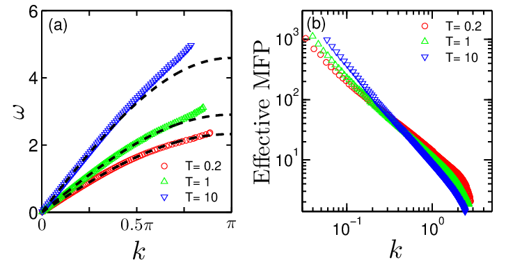
(i) Firstly, for all frequencies depicted, the phase perfectly decreases linearly with . This corroborates the existence of a-ph’s with a corresponding wavenumber . We evaluate for different driving frequencies , as depicted in Fig. 4(a), and compare our results with predictions taken from renormalized phonon theory (dashed lines) [14, 15], which predicts
| (22) |
Here, denotes the temperature-dependent renormalization factor that quantifies the strength of nonlinearity. The temperature dependent sound speed emerges as . For the FPU- lattice [14, 15]; it increases with temperature, starting out at . As seen in Fig. 4(a), excellent agreement is obtained for low frequency a-ph’s. The differences between the a-ph concept and renormalized phonon theory occur at large frequencies, with deviations slightly increasing with increasing temperature. This corroborates with the fact that effective phonon theory self-consistently applies to weak anharmonic forces and long wavelength phonons only.
(ii) Secondly, within the depicted frequency regime the amplitude , Fig. 3(c), perfectly decays exponentially with increasing . Therefore, a sensible MFP is obtained for each a-ph, cf. in Fig. 4(b), where we depict the MFPs at three different ambient temperatures. Moreover, the MFPs diverge with the decreasing wavenumber . This is a salient feature known for momentum conserving 1D systems [39].
Interestingly, a power-law divergence with is observed for small for various temperatures. The numerical result closely matches the prediction of Peierls–Boltzmann theory at weak anharmonic nonlinearity, rendering [19, 40, 41]. A divergent exponent causes an anomalous divergent heat conductivity with [19, 8]. Therefore, we numerically find , which is close to results in [38, 42].
IV.2 FPU- lattice.


The FPU- lattices containing a non-vanishing cubic term and distinctly differ from FPU- lattices. The inherent asymmetry of the interaction potential yields a nonvanishing internal pressure [43, 44]. Figure 5 depicts the response function for the FPU- lattice.
As shown in Fig. 5(b), the perfect linear dependence of the phases on can still be observed. Therefore, it corroborates the existence of a-ph’s in the FPU- case.
The amplitudes , as shown in Fig. 5(c), however, deviate from an exponential decay but instead depict multiple scales. Therefore, a strict MFP cannot be defined. Interestingly, as depicted as an example in Fig. 5(a), their behavior can be fitted with a stretched exponential
| (23) |
with a frequency dependent parameter . Therefore, an effective single scale can still be defined for each frequency if we average over all scales, i.e.,
| (24) |
where is the Gamma function. The dispersion relation and the so obtained effective MFPs are displayed in Fig. 6.
Although a renormalized phonon theory for FPU- lattices does not exist, we still find that Eq. (22) holds approximately true for the dispersion of our a-ph’s, see the dashed lines in Fig. 6. The corresponding sound speed matches well a recent result in [45], which reads
| (25) |
where is the potential, denotes the covariance for any two quantities and , and is the internal pressure.
IV.3 -lattice.
Here, the inter-particle potential is together with an on-site potential . For this momentum-nonconserving nonlinear lattice we still find that the phase follows a perfect linear decay. Moreover, the corresponding MFP for the a-ph exists with a single scale, i.e., nicely decays exponentially (figures for are similar to Fig. (3) so they are not shown here).

Our proposed a-ph concept holds up also in the presence of an onsite interaction. The dispersion relation and the related MFPs are depicted in Fig. 7. Consistent with the validity of Fourier’s law for momentum non-conserving systems the long wavelength phonons exhibit finite MFPs [46, 47]. Our result for the dispersion relation agrees well with the renormalized phonon theory [48], namely,
| (26) |
V Summary and discussion.
The challenge of identifying phonon excitations in strongly nonlinear lattices beyond their corresponding harmonic approximation, termed here anharmonic phonons (a-ph’s), has been tackled with MD via a theoretically imposed “tuning fork experiment”. Doing so enables one to account for the role of temperature, large frequencies and lattice nonlinearity in the strong nonlinearity regime. This experiment-inspired phonon concept has been successfully tested over extended parameter regimes of frequency and temperature for three archetype 1D nonlinear lattice models. Note that a temperature dependent phonon MFP is typically not accessible with prior theories without making reference to additional assumptions [16, 17, 18, 19]. Physically, the MFP relates to a phonon transport relaxation time which generally does not equal the phonon lifetime [30].
Our concept for the MFP holds up beyond the validity regime of renormalized phonon theories [10, 11, 12, 13, 14, 15], depicting a single, exponentially decaying scale for both the FPU- lattice, exhibiting anomalous heat conduction, and the lattice, exhibiting a Fourier’s law behavior. The case of the FPU- lattice turned out intriguing in that the MFPs no longer exhibit a single scale but decay with multiple scales.
A hallmark of our scheme is that the existence of the a-ph’s and their MFPs is not postulated a priori, but instead is physically corroborated by following the propagation of traveling waves with an experiment. The outcome then either validates, or possibly also invalidates, the existence of a-ph with a finite MFP. Our scheme thus distinctly differs from existing phonon quasiparticle concepts [20, 21, 22, 23, 24, 26, 27]. A most characteristic feature within our scheme is that here we directly search for the existence of an a-ph MFP.
The presented a-ph concept allows one to characterize as well infinite MFPs and multiple spatial decay scales, all being features that crucially impact anomalous thermal transport in low-dimensional systems. This a-ph concept may as well spur interest in describing heat transport in 3D materials, encompassing engineered complex materials, such as phononic metamaterials [49, 50, 51].
Acknowledgements.
This work is supported by R-144-000-305-112 from MOE T2 (Singapore). The authors would like to thank Dr. N. Li and Dr. J. Ren for useful discussions.References
- [1] M. Born and K. Huang, Dynamical Theory of Crystal Lattices (Oxford University Press, Oxford, 1954).
- [2] R. E. Peierls, Ann. Phys. (N.Y.) 3, 1055 (1929).
- [3] R. E. Peierls, Quantum Theory of Solids (Oxford University Press, London, 1955).
- [4] J. M. Ziman, Principles of the theory of solids, 2nd ed. (Cambridge University Press, Cambridge, 1972).
- [5] Z. Rieder, J. L. Lebowitz, and E. Lieb, J. Math. Phys. 8, 1073 (1967).
- [6] D. Segal, A. Nitzan and P. Hänggi, J. Chem. Phys. 119, 6840 (2003).
- [7] S. Lepri, R. Livi, and A. Politi, Phys. Rep. 377, 1 (2003).
- [8] A. Dhar, Adv. Phys. 57, 457 (2008).
- [9] S. Liu, X. Xu, R. Xie, G. Zhang and B. Li, Eur. Phys. J. B 85, 337 (2012).
- [10] C. Alabiso, M. Casartelli, and P. Marenzoni, J. Stat. Phys. 79, 451 (1995).
- [11] C. Alabiso and M. Casartelli, J. Phys. A 34, 1223 (2001).
- [12] B. Gershgorin, Y. V. Lvov, and D. Cai, Phys. Rev. Lett. 95, 264302 (2005).
- [13] B. Gershgorin, Y. V. Lvov, and D. Cai, Phys. Rev. E 75, 046603 (2007).
- [14] N. Li, P. Tong, and B. Li, Europhys. Lett. 75, 49 (2006).
- [15] N. Li, B. Li, and S. Flach, Phys. Rev. Lett. 105, 054102 (2010).
- [16] J. Callaway, Phys. Rev. 113, 1046 (1959).
- [17] M. Holland, Phys. Rev. 132, 2461 (1963).
- [18] C. Herring, Phys. Rev. 95, 954 (1954).
- [19] A. Pereverzev, Phys. Rev. E 68, 056124 (2003).
- [20] A. Henry and G. Chen, J. Comput. Theor. Nanosci. 5, 141 (2008)
- [21] J. E. Turney, E. S. Landry, A. J. H. McGaughey and C. H. Amon, Phys. Rev. B 79, 064301 (2009).
- [22] J. A. Thomas, J. E. Turney, R. M. Iutzi, C. H. Amon and A. J. H. McGaughey, Phys. Rev. B 81, 081411(R) (2010).
- [23] T. Sun, X. Shen and P. B. Allen, Phys. Rev. B 82, 224304 (2010).
- [24] D.–B. Zhang, T. Sun and R. M. Wentzcovitch, Phys. Rev. Lett. 112, 058501 (2014).
- [25] A. Maradudin and A. Fein, Phys. Rev. 128, 2589 (1962).
- [26] W. M. Collins and H. R. Glyde, Phys. Rev. B 18, 1132 (1978).
- [27] P. M. Chaikin and T. C. Lubensky, Principles of Condensed Matter Physics, (Cambridge University Press, Cambridge, 2000), see Sect. 7.7.
- [28] J. W. L. Pang, W. J. L. Buyers, A. Chernatynskiy, M. D. Lumsden, B. C. Larson and S. R. Phillpot, Phys. Rev. Lett. 110, 157401 (2013).
- [29] A. Ward and D. A. Broido, Phys. Rev. B 81, 085205 (2010).
- [30] T. Sun and P. B. Allen, Phys. Rev. B 82, 224305 (2010).
- [31] P. Hänggi and H. Thomas, Phys. Rep. 88, 207 (1982).
- [32] Following the Appendix in Ref. [33], we choose the atom mass , the lattice constant , the force constant and the Boltzmann constant as the four basic units to scale all physical quantities involved to dimensionless quantities.
- [33] N. Li, J. Ren, L. Wang, G. Zhang, P. Hänggi, and B. Li, Rev. Mod. Phys. 84, 1045 (2012).
- [34] R. Kubo, M. Toda, and N. Hashitsume, Statistical Physics II (Springer, Berlin, 1991).
- [35] J. Laskar and P. Robutel, Celest. Mech. Dyn. Astron. 80, 39 (2001).
- [36] J. Ford, Phys. Rep. 213, 271 (1992).
- [37] G. P. Berman and F. M. Izrailev, Chaos 15, 015104 (2005).
- [38] S. Lepri, R. Livi, and A. Politi, Phys. Rev. Lett. 78, 1896 (1997).
- [39] S. Lepri, R. Livi, and A. Politi, Europhys. Lett. 43, 271 (1998).
- [40] B. Nickel, J. Phys. A: Math. and Theor. 40, 1219 (2007).
- [41] J. Lukkarinen and H. Spohn, Comm. Pure Appl. Math. 61, 1753 (2008).
- [42] L. Wang and T. Wang, Europhys. Lett. 93, 54002 (2011).
- [43] Y. Zhong, Y. Zhang, J. Wang, and H. Zhao, Phys. Rev. E 85, 060102 (2012).
- [44] L. Wang, B. Hu, and B. Li, Phy. Rev. E 88, 052112 (2013).
- [45] H. Spohn, J. Stat. Phys. 154, 1191 (2014): see Eq. (8.32) therein.
- [46] B. Hu, B. Li, and H. Zhao, Phys. Rev. E 61, 3828 (2000).
- [47] K. Aoki and D. Kusnezov, Phys. Lett. A 265, 250 (2000).
- [48] N. Li and B. Li, Phys. Rev. E 87, 042125 (2013).
- [49] J. K. Yu, S. Mitrovic, D. Tham, J. Varghese, and J. R. Heath, Nat. Nanotechnol. 5, 718 (2010).
- [50] L. Yang, N. Yang and B. Li, Nano Lett., 14, 1734 (2014).
- [51] B. L. Davis and M. I. Hussein, Phys. Rev. Lett. 112, 055505 (2014).