Medium effects on the thermal conductivity of a hot pion gas

The observation of large elliptic flow of hadrons in heavy ion collisions at RHIC has led to the description of quark-gluon plasma as a nearly perfect fluid [1]. This interpretation is based on the small but finite value of the shear viscosity to entropy density ratio required in a relativistic hydrodynamic description of the collision. The effects of dissipation on the dynamical evolution of matter produced in relativistic heavy ion collisions have thus been a major topic of discussion in recent times [2]. At the microscopic level dissipative phenomena are studied by considering small departures from equilibrium. In kinetic theory the transport of momenta and heat as a result of collisions is quantitatively expressed in terms of coefficients of viscosity and thermal conductivity [3, 4]. A large number of studies on the viscous coefficients have been performed in the transport approach. The shear viscosity $\eta$ has been most commonly discussed followed by the bulk viscosity $\zeta$, both for partonic as well as hadronic systems [5, 6, 7, 8, 9, 10, 11, 12, 13, 14, 15, 16, 17, 18, 19, 20, 21, 22, 23, 24, 25]. The interesting issue concerning the behaviour of the viscosities in the vicinity of the transition from partonic to hadronic matter have also been discussed [1, 18, 12, 14, 15, 19, 20]. While the value of $\eta/s$ is expected to go through a minimum near the critical temperature [1, 18], $\zeta/s$ is believed to be large or diverging [12, 15, 19] at or near the transition.

The effects of heat flow in heavy ion collisions has received much less attention. This is presumably on account of the fact that the net baryon number in the central rapidity region at the RHIC and LHC is very small. However, at FAIR energies or in the low energy runs at RHIC the baryon chemical potential is expected to be significant and heat conduction by baryons may play a more important role. On the other hand, a thermal system consisting of pions can sustain heat conduction despite the fact that the pions themselves do not carry baryon number [5]. This is due to the fact that the total number of pions in heavy ion collisions is essentially conserved. Pion number changing reactions are not sustained towards the late stages where collisions are mostly elastic and the system undergoes chemical freezeout. As the system expands and cools a pion chemical potential develops in order to keep the pion number fixed. Based on such a scenario a few studies of heat conduction by pions have been carried out. Using the experimental $\pi\pi$ cross-section the thermal conductivity of a pion gas was estimated in [5, 6, 7] whereas in [22] a unitarized scattering amplitude was employed. The heat conductivity was also obtained using the Kubo formula in [13, 23, 26]. For the case of a classical gas, heat flow has been studied recently in a transport model [24] and a fluid-dynamical theory was derived [25]. Investigating the effect of thermal conductivity on first order phase transitions, non-trivial fluctuation effects were observed in [27] which may result in a non-monotonic behaviour of certain observables as a function of collisional energy and may be seen from experimental analysis at RHIC and FAIR. A clear picture of the behaviour of thermal conductivity in the vicinity of a phase transition is however yet to emerge.

In the kinetic theory approach the dynamics of interaction resides in the differential cross-section which goes as an input. In almost all estimations of the transport coefficients a vacuum cross-section was employed. In [28, 29] a medium dependent cross-section was used in the evaluation of shear and bulk viscosities of a pion gas which resulted in a significant deviation from the results obtained with the $\pi\pi$ cross-section in vacuum.

In this work we study the temperature dependence of the thermal conductivity of a pion gas. In particular, our intention is to emphasize on the effect of the medium on its temperature dependence brought in by the cross-section. To this end we employ an effective Lagrangian approach in which the $\pi\pi$ scattering amplitude is obtained in terms of $\rho$ and $\sigma$ meson exchange. Medium effects are then incorporated by introducing in-medium propagators dressed by one loop self energies calculated in the framework of thermal field theory. We use a temperature dependent pion chemical potential and obtain the thermal conductivity for temperatures in the range between chemical and kinetic freezeout in heavy ion collisions.

The thermal conductivity $\lambda$ is obtained by solving the Uehling-Uhlenbeck equation in the Chapman-Enskog approximation to first order. This calculation is performed along the lines of [30, 7] and is described elaborately in [29]. Here we provide only the basics of the formalism. We start with the transport equation for the phase-space distribution $f(x,p)$ of a relativistic pion gas which is given by

$$p^{\mu}\partial_{\mu}f(x,p)=C[f]~.$$

(1)

For binary elastic collisions $p+k\to p^{\prime}+k^{\prime}$, the collision term $C[f]$ is defined by,

	$\displaystyle C[f]=$		$\displaystyle\frac{1}{2}\int d\Gamma_{k}\ d\Gamma_{p^{\prime}}\ d\Gamma_{k^{\prime}}[f(x,p^{\prime})f(x,k^{\prime})\{1+f(x,p)\}$		(2)
			$\displaystyle\times\{1+f(x,k)\}-f(x,p)f(x,k)\{1+f(x,p^{\prime})\}$
			$\displaystyle\times\{1+f(x,k^{\prime})\}]\ W$

where,

$$W=(2\pi)^{4}\delta^{4}(p+k-p^{\prime}-k^{\prime})\frac{1}{2}|{\cal M}|^{2},\,\,\,d\Gamma_{q}=\frac{d^{3}q}{(2\pi)^{3}2E_{q}}~.$$

For a pion gas slightly away from equilibrium the phase space distribution function can be expanded in the first Chapman-Enskog approximation as

$$f(x,p)=f^{(0)}(x,p)+f^{(0)}(x,p)[1+f^{(0)}(x,p)]\phi(x,p),$$

(3)

where, $f^{(0)}(x,p)=[e^{\frac{p\cdot u(x)-\mu(x)}{T(x)}}-1]^{-1}$ is the local equilibrium Bose distribution function. The deviation function $\phi(x,p)$ then satisfies the following linearized transport equation

$$p^{\mu}\partial_{\mu}f^{(0)}(x,p)=-{\cal L}[\phi]~$$

(4)

in which the collision term is given by,

	$\displaystyle{\cal L}[\phi]$	$\displaystyle=$	$\displaystyle f^{(0)}(x,p)\frac{1}{2}\int d\Gamma_{k}\ d\Gamma_{p^{\prime}}\ d\Gamma_{k^{\prime}}f^{(0)}(x,k)$		(5)
		$\displaystyle\times$	$\displaystyle\{1+f^{(0)}(x,p^{\prime})\}\{1+f^{(0)}(x,k^{\prime})\}$
		$\displaystyle\times$	$\displaystyle[\phi(x,p)+\phi(x,k)-\phi(x,p^{\prime})-\phi(x,k^{\prime})]\ W~.$

To solve this equation $\phi$ is generally expressed in the form

$$\phi=A\partial_{\nu}u^{\nu}+B_{\mu}\Delta^{\mu\nu}(T^{-1}\partial_{\nu}T-Du_{\nu})-C_{\mu\nu}\langle\partial^{\mu}u^{\nu}\rangle$$

(6)

where $D=u^{\mu}\partial_{\mu}$ and $\Delta^{\mu\nu}=g^{\mu\nu}-u^{\mu}u^{\nu}$, $u^{\mu}$ being the flow velocity. The scalar and tensor processes denoted by the first and third terms are connected with bulk and shear viscosities respectively. The vector process given by the second term corresponds to the transport phenomena related to thermal conduction. Comparing with the expression for energy 4-flow, $I^{\mu}=\lambda(\partial_{\sigma}T-TDU_{\sigma})\Delta^{\mu\sigma}$ the coefficient of thermal conductivity $\lambda$ can be defined as

$$\lambda=\frac{2}{3T}\int d\Gamma_{p}f^{(0)}(1+f^{(0)})B_{\nu}p^{\nu}(p\cdot u-h)$$

(7)

where $h$ is the enthalpy per particle. The unknown coefficient $B_{\mu}=B\Delta_{\mu\nu}p^{\nu}$ can be obtained by solving the equation,

$${\cal L}[B_{\mu}]=-\frac{1}{T}f^{(0)}(1+f^{(0)})\Delta_{\mu\nu}p^{\nu}(p\cdot u-h)~.$$

(8)

Here we follow the procedure outlined in [30, 7] in which $B_{\mu}$ is expanded in terms of orthogonal Laguerre polynomials of order $3/2$. After some simplifications (discussed in detail in Refs. [7, 29]) the first approximation to thermal conductivity comes out to be,

$$\lambda=\frac{T}{3m_{\pi}}\frac{\beta_{1}^{2}}{b_{11}}$$

(9)

where,

	$\displaystyle\beta_{1}$	$\displaystyle=$	$\displaystyle-3z^{2}\left\{1+5z^{-1}\frac{S^{2}_{3}(z)}{S^{1}_{2}(z)}-\left(\frac{S^{1}_{3}(z)}{S^{1}_{2}(z)}\right)^{2}\right\}$
	$\displaystyle b_{11}$	$\displaystyle=$	$\displaystyle I_{1}(z)+I_{2}(z)~~{\rm with}~~z=m_{\pi}/T~.$		(10)

The integrals $I_{\alpha}(z)$ are given by [28, 29]

	$\displaystyle I_{\alpha}(z)$	$\displaystyle=$	$\displaystyle\frac{8z^{5}}{[S_{2}^{1}(z)]^{2}}\ e^{(-2\mu_{\pi}/T)}\int_{0}^{\infty}d\psi\ \cosh^{3}\psi\sinh^{7}\psi$
		$\displaystyle\times$	$\displaystyle\int_{0}^{\pi}d\Theta\sin\Theta\{\frac{1}{2}\frac{d\sigma}{d\Omega}\}(\psi,\Theta)\int_{0}^{2\pi}d\phi$
		$\displaystyle\times$	$\displaystyle\int_{0}^{\infty}d\chi\sinh^{(2\alpha+2)}\chi\int_{0}^{\pi}d\theta\sin\theta$
		$\displaystyle\times$	$\displaystyle\frac{e^{2z\cosh\psi\cosh\chi}}{(e^{E}-1)(e^{F}-1)(e^{G}-1)(e^{H}-1)}\ M_{\alpha}(\theta,\Theta),$

and $S_{n}^{\alpha}(z)$ denotes integrals over Bose functions which can be expressed in terms of infinite series as $S_{n}^{\alpha}(z)=\displaystyle\sum_{k=1}^{\infty}e^{k\mu/T}k^{-\alpha}K_{n}(kz)$, $K_{n}(x)$ denoting the modified Bessel function of order $n$. The exponents in the Bose functions and the functions $M_{\alpha}(\theta,\Theta)$ are respectively given by

	$\displaystyle E$	$\displaystyle=$	$\displaystyle z(\cosh\psi\cosh\chi-\sinh\psi\sinh\chi\cos\theta)-\mu_{\pi}/T$
	$\displaystyle F$	$\displaystyle=$	$\displaystyle z(\cosh\psi\cosh\chi-\sinh\psi\sinh\chi\cos\theta^{\prime})-\mu_{\pi}/T$
	$\displaystyle G$	$\displaystyle=$	$\displaystyle E+2z\sinh\psi\sinh\chi\cos\theta$
	$\displaystyle H$	$\displaystyle=$	$\displaystyle F+2z\sinh\psi\sinh\chi\cos\theta^{\prime}~,$		(12)

	$\displaystyle M_{1}(\theta,\Theta)$	$\displaystyle=$	$\displaystyle\cos^{2}\theta+\cos^{2}\theta^{\prime}-2\cos\theta\cos\theta^{\prime}\cos\Theta~,$
	$\displaystyle M_{2}(\theta,\Theta)$	$\displaystyle=$	$\displaystyle[\cos^{2}\theta-\cos^{2}\theta^{\prime}]^{2}$		(13)

where $\cos\theta^{\prime}=\cos\theta\cos\Theta-\sin\theta\sin\Theta\cos\phi~.$

The $\pi\pi$ cross-section is the key dynamical input for evaluating transport coefficients. Here the scattering is assumed to proceed via $\sigma$ and $\rho$ meson exchange in the medium. From the effective interaction [31]

$${\cal L}=g_{\rho}\vec{\rho}^{\mu}\cdot\vec{\pi}\times\partial_{\mu}\vec{\pi}+\frac{1}{2}g_{\sigma}m_{\sigma}\vec{\pi}\cdot\vec{\pi}\sigma$$

(14)

the matrix elements for $\pi\pi$ scattering are given by the following expressions where the widths of the $\sigma$ and $\rho$ mesons have been introduced in the propagators involved in the corresponding $s$-channel processes. We thus have

	$\displaystyle{\cal M}_{I=0}$	$\displaystyle=$	$\displaystyle 2g_{\rho}^{2}\left[\frac{s-u}{t-m_{\rho}^{2}}+\frac{s-t}{u-m_{\rho}^{2}}\right]$
		$\displaystyle+$	$\displaystyle g_{\sigma}^{2}m_{\sigma}^{2}\left[\frac{3}{s-m_{\sigma}^{2}+im_{\sigma}\Gamma_{\sigma}}+\frac{1}{t-m_{\sigma}^{2}}+\frac{1}{u-m_{\sigma}^{2}}\right]$
	$\displaystyle{\cal M}_{I=1}$	$\displaystyle=$	$\displaystyle g_{\rho}^{2}\left[\frac{2(t-u)}{s-m_{\rho}^{2}+im_{\rho}\Gamma_{\rho}}+\frac{t-s}{u-m_{\rho}^{2}}-\frac{u-s}{t-m_{\rho}^{2}}\right]$		(15)
		$\displaystyle+$	$\displaystyle g_{\sigma}^{2}m_{\sigma}^{2}\left[\frac{1}{t-m_{\sigma}^{2}}-\frac{1}{u-m_{\sigma}^{2}}\right]~.$

Defining the isospin averaged amplitude as $|{\cal M}|^{2}=\frac{1}{9}\sum_{I}|{\cal M}_{I}|^{2}$ and ignoring the non-resonant $I=2$ contribution, the cross-section is found to agree very well [28, 29] with the estimate based on measured phase-shifts given in [6]. In this way it is ensured that the dynamical model is normalized against experimental data although, this approach of introducing the width is not quite in agreement with low energy theorems based on chiral symmetry.

To obtain the in-medium cross-section we replace the vacuum width in the above expressions by the ones in the medium. The width is related to the imaginary part of the self-energy through the relation [32]

$$\Gamma(T,M)=-M{\rm Im}\Pi(T,M)$$

(16)

where $\Pi$ denotes the one-loop self energy diagrams shown in fig. 1 and are evaluated using the real-time formalism of thermal field theory. The $\sigma$ meson self-energy is obtained from the $\pi\pi$ loop diagram whereas in case of the $\rho$ meson the $\pi\pi$, $\pi\omega$, $\pi h_{1}$, $\pi a_{1}$ graphs are evaluated using interactions from chiral perturbation theory [33]. The longitudinal and transverse parts of the $\rho$ self-energy are defined as [34]

$$\Pi^{T}=-\frac{1}{2}(\Pi_{\mu}^{\mu}+\frac{q^{2}}{\bar{q}^{2}}\Pi_{00}),~~~~\Pi^{L}=\frac{1}{\bar{q}^{2}}\Pi_{00},~~~\Pi_{00}\equiv u^{\mu}u^{\nu}\Pi_{{\mu\nu}}~.$$

(17)

The momentum dependence being weak we take an average over the polarizations. The imaginary part of the self-energy obtained by evaluating the loop diagrams is given by [35]

	$\displaystyle{\rm Im}\Pi(q_{0},\vec{q})=-\pi\int\frac{d^{3}k}{(2\pi)^{3}4\omega_{\pi}\omega_{h}}\times$
	$\displaystyle\left[N_{1}\{(1-f^{(0)}(\omega_{\pi})-f^{(0)}(\omega_{h}))\delta(q_{0}-\omega_{\pi}-\omega_{h})\right.$
	$\displaystyle+(f^{(0)}(\omega_{\pi})-f^{(0)}(\omega_{h}))\delta(q_{0}-\omega_{\pi}+\omega_{h})\}+$
	$\displaystyle N_{2}\{(f^{(0)}(\omega_{h})-f^{(0)}(\omega_{\pi}))\delta(q_{0}+\omega_{\pi}-\omega_{h})$
	$\displaystyle\left.-(1-f^{(0)}(\omega_{\pi})-f^{(0)}(\omega_{h}))\delta(q_{0}+\omega_{\pi}+\omega_{h})\}\right]$		(18)

where $f^{(0)}(\omega)=\frac{1}{e^{(\omega-\mu_{\pi})/T}-1}$ is the Bose distribution function with arguments $\omega_{\pi}=\sqrt{\vec{k}^{2}+m_{\pi}^{2}}$ and $\omega_{h}=\sqrt{(\vec{q}-\vec{k})^{2}+m_{h}^{2}}$. The terms $N_{1}$ and $N_{2}$ stem from the vertex factors and the numerators of vector propagators, details of which can be found in [35]. The angular integration is done using the $\delta$-functions which define the kinematic domains for occurrence of scattering and decay processes which lead to loss or gain of $\rho$ (or $\sigma$) mesons in the medium. To account for the substantial $3\pi$ and $\rho\pi$ branching ratios of the heavy particles in the loop the self-energy function is convoluted with their widths,

	$\displaystyle\Pi(q,m_{h})$	$\displaystyle=$	$\displaystyle\frac{1}{N_{h}}\int^{(m_{h}+2\Gamma_{h})^{2}}_{(m_{h}-2\Gamma_{h})^{2}}dM^{2}\,\times$		(19)
			$\displaystyle\frac{1}{\pi}{\rm Im}\left[\frac{1}{M^{2}-m_{h}^{2}+iM\Gamma_{h}(M)}\right]\Pi(q,M)$

with

	$\displaystyle N_{h}$	$\displaystyle=$	$\displaystyle\displaystyle\int^{(m_{h}+2\Gamma_{h})^{2}}_{(m_{h}-2\Gamma_{h})^{2}}dM^{2}\,\times$		(20)
			$\displaystyle\frac{1}{\pi}{\rm Im}\left[\frac{1}{M^{2}-m_{h}^{2}+iM\Gamma_{h}(M)}\right]~.$

The contribution from the loops with these unstable particles can thus be looked upon as multi-pion effects in $\pi\pi$ scattering.

It is generally accepted [36] that the hadronic gas produced after the transition is in chemical equilibrium where the chemical potential of pions for example is zero. Chemical freezeout for an evolving hadronic gas occurs much earlier than kinetic freezeout. The number-changing inelastic collisions cease at chemical freezeout and the total pion number becomes fixed. Thereafter only elastic collisions take place until the pions actually decouple later at kinetic freezeout. The pion chemical potential consequently grows from zero to a maximum at kinetic freezeout so as to keep the total number of pions fixed. Here the temperature-dependent pion chemical potential is taken from Ref. [37] which implements the above scenario and is parametrized as

$$\mu_{\pi}(T)=a+bT+cT^{2}+dT^{3}$$

(21)

with $a=0.824$, $b=3.04$, $c=-0.028$, $d=6.05\times 10^{-5}$ and $T$, $\mu_{\pi}$ in MeV.

We now plot in fig. 2 the total $\pi\pi$ cross-section defined by $\sigma(s)=\frac{1}{2}\int d\Omega\frac{d\sigma}{d\Omega}$ with $\frac{d\sigma}{d\Omega}=\frac{|{\cal M}|^{2}}{64\pi^{2}s}$. The increase in the widths of the exchanged $\rho$ and $\sigma$ on account of thermal emission and absorption is reflected in a significant change in both the magnitude and shape of the cross-section as a function of the c.m. energy. A rough estimate of the mean free path of pions using the peak value of the in-medium cross-section comes out to be $\sim$ 1-2 fm at $T=160$ MeV. A macroscopic length scale such as the typical size of the system at this stage being much larger justifies the use of the Chapman-Enskog method for solving the transport equation.

We next turn to the results of thermal conductivity. In fig. 3 we plot $\lambda T$ as a function of $T$ evaluated in the Chapman-Enskog approach. The dashed line shows results where the vacuum cross-section is used in the integrals (). For a vanishing pion chemical potential this result agrees with those of [6, 7]. Replacing the vacuum widths by the in-medium widths in the $\rho$ and $\sigma$ propagators in the scattering amplitudes results in the long dashed line. A substantial medium effect is seen even for $\mu_{\pi}=0$ and this is seen to increase with increase of temperature. We now introduce the temperature dependent $\mu_{\pi}$ both in the cross-section and elsewhere in eqs. (10) and (). This yields the solid line. On comparing with the long-dashed line the effect of chemical freeze-out is seen to be more at lower temperatures since the value of $\mu_{\pi}(T)$ increases as one approaches kinetic freeze-out.

At this stage it is worthwhile to compare the results with those obtained using the so-called relaxation time approximation. This method is the simplest way to linearize the transport equation and is widely used. In this approach the distribution function $f(x,p)$ is assumed to go over to the equilibrium distribution $f^{(0)}(x,p)$ over a time scale usually referred to as the relaxation time $\tau(p)$ which is actually given by the inverse of the collision frequency $\omega(p)$. For a binary elastic collision $\pi(p)+\pi(k)\to\pi(p^{\prime})+\pi(k^{\prime})$ it is given by

	$\displaystyle\omega(p)=$		$\displaystyle\int d\Gamma_{k}\frac{\sqrt{s(s-4m_{\pi}^{2})}}{E_{p}}f^{(0)}(E_{k})(1+f^{(0)}(E_{p^{\prime}}))$		(22)
			$\displaystyle\times(1+f^{(0)}(E_{k^{\prime}}))\sigma(s)~.$

We plot in fig. 4 the mean (thermal averaged) relaxation time as a function of temperature. This is given by $\tau(T,\mu_{\pi})=1/\overline{\omega}(T,\mu_{\pi})$ where

$$\overline{\omega}(T,\mu_{\pi})=\int d^{3}pf^{(0)}(p)\omega(p)/\int d^{3}pf^{(0)}(p)~.$$

(23)

The lower set of curves with filled circles correspond to a temperature dependent chemical potential. The large difference with the upper set of curves depicting the situation at vanishing pion chemical potential especially at lower temperatures shows the role played by $\mu_{\pi}$. Accounting for the isospin degeneracy, the vacuum result for $\mu_{\pi}=0$ agrees with the estimate of [6, 7]. The solid line in both cases show a noticeable medium effect compared to the vacuum.

It may be pointed out that the mean relaxation time characterizes the rate of change of the distribution function due to collisions and only serves as a orientational guide to equilibrium [6]. On the other hand the relaxation time of flows give the time scales over which momenta and heat are transported. They cannot be obtained in the Chapman-Enskog formalism where the neglect of all gradients of flows in the conservation laws lead to infinite speeds for the flows [7].

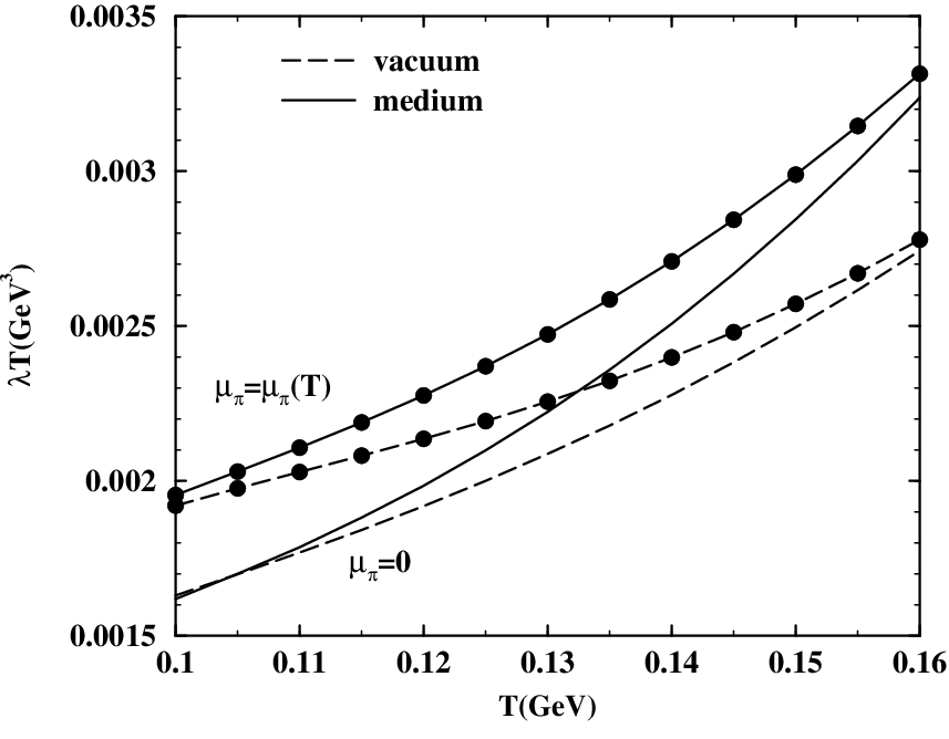
The transport equation in the relaxation time approximation reduces to

$$\frac{\partial f}{\partial t}+\vec{v}_{p}\cdot\vec{\nabla}f=-\frac{(f-f^{(0)})}{\tau}.$$

(24)

from which the thermal conductivity comes out to be [5],

$$\lambda=\frac{2}{3T^{2}}\int d\Gamma_{p}\frac{p^{2}}{E_{p}}(E_{p}-h)^{2}\tau(p)f^{(0)}(E_{p})(1+f^{(0)}(E_{p})).$$

(25)

In fig. 5 we have plotted $\lambda T$ versus $T$ both for zero and a temperature dependent chemical potential. The substantial effect of the medium is distinctly visible through the difference between the dashed and solid lines in the two sets. The separation between the set of curves with and without circles shows the effect of the pion chemical potential and as expected, is more at lower temperatures.

The value of $\lambda$ for the various cases displayed in figs. 3 and 5 lie within $\sim$0.4-1.2 in units of fm^-2 at $T=160$ MeV. Taking the peak value of the $\pi\pi$ cross-section as shown in fig. 2 these values are within reasonable agreement with those of [24].

To summarize, we have evaluated the thermal conductivity of an interacting pion gas by solving the relativistic transport equation in the Chapman-Enskog and relaxation time approximations. In-medium effects on the $\pi\pi$ cross-section are incorporated through one-loop self-energies of the exchanged $\rho$ and $\sigma$ mesons calculated using thermal field theory. The effect of chemical freezeout is incorporated through a temperature dependent pion chemical potential which keeps the pion number conserved. It is observed that the temperature dependence of the thermal conductivity is significantly affected. It will be interesting to observe the consequences on the evolution of the late stages of heavy ion collisions by including it in fluid-dynamical simulations.

It may be pointed out that a realistic hadron gas is composed of several types of hadrons and in principle should be considered for the evaluation of transport coefficients. However, treating the $\pi N$ gas as a binary hadronic mixture the viscosities and thermal conductivities were found [6] to be close to those of a pion gas due to the small concentration of nucleons. It may be worthwhile to investigate the role of medium effects in such systems especially for situations involving high baryon density.

References

- [1] L. P. Csernai, J. I. Kapusta and L. D. McLerran, Phys. Rev. Lett. 97, 152303 (2006).
- [2] T. Ullrich, B. Wyslouch and J. W. Harris, Proceedings of Quark Matter 2012 (QM 2012), Washington, DC, USA, August 13-18, 2012, Nucl. Phys. A 904-905 (2013) pp. 1c.
- [3] S. R. De Groot, W. A. Van Leeuwen and C. G. Van Weert, Relativistic Kinetic Theory, Principles And Applications Amsterdam, Netherlands: North-holland (1980).
- [4] D. N. Zubarev, Non-equilibrium Statistical Thermodynamics (Consultants Bureau, NY, 1974).
- [5] S. Gavin, Nucl. Phys. A 435 (1985) 826.
- [6] M. Prakash, M. Prakash, R. Venugopalan and G. Welke, Phys. Rept. 227 (1993) 321.
- [7] D. Davesne, Phys. Rev. C 53, 3069 (1996).
- [8] A. Dobado and S. N. Santalla, Phys. Rev. D 65, 096011 (2002).
- [9] A. Dobado and F. J. Llanes-Estrada, Phys. Rev. D 69, 116004 (2004).
- [10] J. W. Chen, Y. H. Li, Y. F. Liu and E. Nakano, Phys. Rev. D 76, 114011 (2007)
- [11] K. Itakura, O. Morimatsu and H. Otomo, Phys. Rev. D 77, 014014 (2008).
- [12] D. Kharzeev and K. Tuchin, JHEP 0809 (2008) 093
- [13] D. Fernandez-Fraile and A. Gomez Nicola, Eur. Phys. J. C 62 (2009) 37.
- [14] A. Dobado, F. J. Llanes-Estrada and J. M. Torres-Rincon, Phys. Rev. D 80 (2009) 114015
- [15] J. -W. Chen and J. Wang, Phys. Rev. C 79 (2009) 044913
- [16] J. Noronha-Hostler, J. Noronha and C. Greiner, Phys. Rev. Lett. 103 (2009) 172302 ; Phys. Rev. C 86 (2012) 024913
- [17] N. Demir and S. A. Bass, Phys. Rev. Lett. 102 (2009) 172302
- [18] C. Sasaki and K. Redlich, Nucl. Phys. A 832 (2010) 62; Phys. Rev. C 79 (2009) 055207.
- [19] D. Fernandez-Fraile and A. Gomez Nicola, Phys. Rev. Lett. 102 (2009) 121601
- [20] A. Dobado and J. M. Torres-Rincon, Phys. Rev. D 86 (2012) 074021
- [21] V. Ozvenchuk, O. Linnyk, M. I. Gorenstein, E. L. Bratkovskaya and W. Cassing, Phys. Rev. C 87 (2013) 064903.
- [22] A. Dobado, F. J. Llanes-Estrada and J. M. Torres Rincon, hep-ph/0702130 [HEP-PH].
- [23] D. Fernandez-Fraile and A. Gomez Nicola, Int. J. Mod. Phys. E 16 (2007) 3010.
- [24] M. Greif, F. Reining, I. Bouras, G. S. Denicol, Z. Xu and C. Greiner,Phys. Rev. E 87 (2013) 033019 .
- [25] G. S. Denicol, H. Niemi, I. Bouras, E. Molnar, Z. Xu, D. H. Rischke and C. Greiner, arXiv:1207.6811 [nucl-th].
- [26] S. Sarkar, Adv. High Energy Phys. 2013 (2013) 627137.
- [27] V. V. Skokov and D. N. Voskresensky, Nucl. Phys. A 847 (2010) 253
- [28] S. Mitra, S. Ghosh and S. Sarkar, Phys. Rev. C. 85, 064917 (2012).
- [29] S. Mitra and S. Sarkar, Phys. Rev. D. 87, 094026 (2013).
- [30] W. A. Van Leeuwen, P. H. Polak and S. R. De Groot, Physica 66, 455 (1973).
- [31] B. D. Serot and J. D. Walecka, Adv. Nucl. Phys. 16, 1 (1986).
- [32] M. Le Bellac, Thermal Field Theory (Cambridge University Press, Cambridge, 1996).
- [33] G. Ecker, J. Gasser, H. Leutwyler, A. Pich and E. de Rafael, Phys. Lett. B 223 (1989) 425.
- [34] S. Ghosh, S. Sarkar and S. Mallik, Eur. Phys. J. C 70, 251 (2010).
- [35] S. Mallik and S. Sarkar, Eur. Phys. J. C 61, 489 (2009).
- [36] H. Bebie, P. Gerber, J. L. Goity and H. Leutwyler, Nucl. Phys. B 378 (1992) 95.
- [37] T. Hirano and K. Tsuda, Phys. Rev. C 66 (2002) 054905