Position-dependent power spectrum of the large-scale structure: a novel method to measure the squeezed-limit bispectrum

Chi-Ting Chiang Affiliation: Max-Planck-Institut für Astrophysik, Karl-Schwarzschild-Str. 1, 85741 Garching, Germany Email: ctchiang@mpa-garching.mpg.de Christian Wagner Affiliation: Max-Planck-Institut für Astrophysik, Karl-Schwarzschild-Str. 1, 85741 Garching, Germany Fabian Schmidt Affiliation: Max-Planck-Institut für Astrophysik, Karl-Schwarzschild-Str. 1, 85741 Garching, Germany Eiichiro Komatsu Affiliation: Max-Planck-Institut für Astrophysik, Karl-Schwarzschild-Str. 1, 85741 Garching, Germany Affiliation: Kavli Institute for the Physics and Mathematics of the Universe, Todai Institutes for Advanced Study, the University of Tokyo, Kashiwa, Japan 277-8583 (Kavli IPMU, WPI)

Abstract

The influence of large-scale density fluctuations on structure formation on small scales is described by the three-point correlation function (bispectrum) in the so-called “squeezed configurations,” in which one wavenumber, say $k_{3}$ , is much smaller than the other two, i.e., $k_{3}\ll k_{1}\approx k_{2}$ . This bispectrum is generated by non-linear gravitational evolution and possibly also by inflationary physics. In this paper, we use this fact to show that the bispectrum in the squeezed configurations can be measured without employing three-point function estimators. Specifically, we use the “position-dependent power spectrum,” i.e., the power spectrum measured in smaller subvolumes of the survey (or simulation box), and correlate it with the mean overdensity of the corresponding subvolume. This correlation directly measures an integral of the bispectrum dominated by the squeezed configurations. Measuring this correlation is only slightly more complex than measuring the power spectrum itself, and sidesteps the considerable complexity of the full bispectrum estimation. We use cosmological $N$ -body simulations of collisionless particles with Gaussian initial conditions to show that the measured correlation between the position-dependent power spectrum and the long-wavelength overdensity agrees with the theoretical expectation. The position-dependent power spectrum thus provides a new, efficient, and promising way to measure the squeezed-limit bispectrum from large-scale structure observations such as galaxy redshift surveys.

1 Introduction

Suppose that we measure a two-point correlation function (power spectrum) of density fluctuations in the Universe. We normally measure this quantity from the entire survey volume in which we have measurements of the matter distribution. Let us divide the survey volume into many subvolumes and measure the power spectrum in each subvolume. In this paper, we show that the power spectrum in each subvolume depends on environment, and is specifically correlated with the mean overdensity of that subvolume. This correlation measures how the small-scale power spectrum responds to the presence of a large-scale density fluctuation, which can be equivalently described by a non-vanishing three-point function (bispectrum).

Even if the initial density fluctuations generated by inflation are perfectly Gaussian, the subsequent non-linear gravitational evolution of matter generates a non-zero bispectrum (see [1] for a review). The “position-dependent power spectrum” thus offers a test of our understanding of structure formation in the Universe. Moreover, improving our understanding of structure formation increases the sensitivity to a small bispectrum generated by inflation, making it possible to test the physics of inflation using observations of the large-scale structure of the Universe.

Not only is this new observable of the large-scale structure of the Universe conceptually straightforward to interpret, but it is also simpler to measure than the full bispectrum. Constraining the physics of inflation using the squeezed-limit bispectrum of the cosmic microwave background is a solved problem [2]. However, doing the same using the bispectrum of the large-scale structure (e.g., distribution of galaxies) is considerably more challenging due to complex survey selection functions as well as to mode couplings caused by the non-linearity of the matter density field as well as the complexity of galaxy formation. This explains why only few measurements of the bispectrum have been reported in the literature [3, 4, 5], and further motivates our use of the position-dependent power spectrum as a simpler route to measuring the squeezed-limit bispectrum. While we mostly have galaxy redshift surveys in mind, this idea can also be applied to the projected matter density as measured through lensing.

In this paper, we study this new observable. We show that the position-dependent power spectrum measures an integral of the bispectrum, which is dominated by the bispectrum in the so-called “squeezed configurations,” in which one wavenumber, say $k_{3}$ , is much smaller than the other two, i.e., $k_{3}\ll k_{1}\approx k_{2}$ . This limit of the bispectrum has a straightforward interpretation (i.e., the large-scale density fluctuation modulating the small-scale power spectrum), which can be predicted using a simple calculation. We restrict ourselves to the position-dependent power spectrum of collisionless particles in real space in this paper. We shall incorporate the effects of halo bias and redshift-space distortions in future publications.

The rest of the paper is organized as follows. In section 2, we derive the relation between the position-dependent power spectrum, the squeezed-limit bispectrum, and the response of small-scale correlations to large-scale overdensities. In section 3, we present measurements of the position-dependent power spectrum from cosmological $N$ -body simulations. In section 4, we compare various theoretical approaches to modeling the position-dependent power spectrum with the simulations. We conclude in section 5. In appendix A, we derive the approximation of the squeezed-limit tree-level matter bispectrum.

2 Position-dependent power spectrum, integrated bispectrum, and linear response function

2.1 Position-dependent power spectrum

Consider a density fluctuation field, $\delta(\mathbf{r})$ , in a big cubic volume with the length of a side $L_{B}$ . For simplicity and a straightforward application to the $N$ -body simulation box, we assume a cubic volume and cubic subvolumes thereof. However, the method is also applicable to realistic survey geometries without major changes. We divide $L_{B}$ into $N_{\rm cut}$ pieces with the length of a side of each subvolume given by $L=L_{B}/N_{\rm cut}$ . In the subvolume centered at $\mathbf{r}_{L}$ , we measure the local mean density perturbation relative to the global mean density of the big volume, $\bar{\delta}(\mathbf{r}_{L})$ , and the position-dependent power spectrum, $P(\mathbf{k},\mathbf{r}_{L})$ . The local mean overdensity within a subvolume centered at $\mathbf{r}_{L}$ is given by

\bar{\delta}(\mathbf{r}_{L})=\frac{1}{V_{L}}\int d^{3}r~\delta(\mathbf{r})W_{L}(\mathbf{r}-\mathbf{r}_{L})~,

(1)

where $\delta(\mathbf{r})$ is the underlying overdensity relative to the global mean density at a position $\mathbf{r}$ and $V_{L}=L^{3}$ is the volume of the subvolume. The window function is given by

W_{L}(\mathbf{x})=\prod_{i=1}^{3}\>\theta(x_{i}),\quad\theta(x_{i})=\left\{\begin{array}[]{cc}1,&|x_{i}|\leq L/2,\\ 0,&\mbox{otherwise}~.\end{array}\right.

(2)

The Fourier transform is $W_{L}(\mathbf{q})=L^{3}\prod_{i=1}^{3}{\rm sinc}(q_{i}L/2)$ , where ${\rm sinc}(x)=\sin(x)/x$ .

We define the position-dependent power spectrum as

P(\mathbf{k},\mathbf{r}_{L})\equiv\frac{1}{V_{L}}|\delta(\mathbf{k},\mathbf{r}_{L})|^{2}\,,

(3)

where $\delta(\mathbf{k},\mathbf{r}_{L})\equiv\int_{V_{L}}d^{3}r~\delta(\mathbf{r})e^{-i\mathbf{r}\cdot\mathbf{k}}$ is the local Fourier transformation of the density fluctuation field. The integral ranges over the subvolume centered at $\mathbf{r}_{L}$ . With this quantity, the mean density perturbation in the subvolume centered at $\mathbf{r}_{L}$ is given by $\bar{\delta}(\mathbf{r}_{L})=(1/V_{L})\delta(\mathbf{k}=0,\mathbf{r}_{L})$ . One can use the window function $W_{L}$ to extend the integration boundaries to infinity

\delta(\mathbf{k},\mathbf{r}_{L})=\int d^{3}r~\delta(\mathbf{r})W_{L}(\mathbf{r}-\mathbf{r}_{L})e^{-i\mathbf{r}\cdot\mathbf{k}}=\int\frac{d^{3}q}{(2\pi)^{3}}~\delta(\mathbf{k}-\mathbf{q})W_{L}(\mathbf{q})e^{-i\mathbf{r}_{L}\cdot\mathbf{q}}~.

(4)

Therefore, the position-dependent power spectrum of the subvolume centered at $\mathbf{r}_{L}$ is

P(\mathbf{k},\mathbf{r}_{L})=\frac{1}{V_{L}}\int\frac{d^{3}q_{1}}{(2\pi)^{3}}\int\frac{d^{3}q_{2}}{(2\pi)^{3}}~\delta(\mathbf{k}-\mathbf{q}_{1})\delta(-\mathbf{k}-\mathbf{q}_{2})W_{L}(\mathbf{q}_{1})W_{L}(\mathbf{q}_{2})e^{-i\mathbf{r}_{L}\cdot(\mathbf{q}_{1}+\mathbf{q}_{2})}~.

(5)

2.2 Integrated bispectrum

Correlating $P(\mathbf{k},\mathbf{r}_{L})$ with the local mean density perturbation of the corresponding subvolume, we find

	$\displaystyle\langle P(\mathbf{k},\mathbf{r}_{L})\bar{\delta}(\mathbf{r}_{L})\rangle$	$\displaystyle=$	$\displaystyle\frac{1}{V_{L}^{2}}\int\frac{d^{3}q_{1}}{(2\pi)^{3}}\int\frac{d^{3}q_{2}}{(2\pi)^{3}}\int\frac{d^{3}q_{3}}{(2\pi)^{3}}~\langle\delta(\mathbf{k}-\mathbf{q}_{1})\delta(-\mathbf{k}-\mathbf{q}_{2})\delta(-\mathbf{q}_{3})\rangle$		(6)
			$\displaystyle~~~~~~~~~~~~~~~~~~~~~~~~~~~\times W_{L}(\mathbf{q}_{1})W_{L}(\mathbf{q}_{2})W_{L}(\mathbf{q}_{3})e^{-i\mathbf{r}_{L}\cdot(\mathbf{q}_{1}+\mathbf{q}_{2}+\mathbf{q}_{3})}~,$		(6)

where $\langle\ \rangle$ denotes the ensemble average over many universes. In the case of a simulation or an actual survey, the average is taken instead over all the subvolumes in the simulation or the survey volume. Through the definition of the bispectrum, $\langle\delta(\mathbf{q}_{1})\delta(\mathbf{q}_{2})\delta(\mathbf{q}_{3})\rangle=B(\mathbf{q}_{1},\mathbf{q}_{2},\mathbf{q}_{3})(2\pi)^{3}\delta_{D}(\mathbf{q}_{1}+\mathbf{q}_{2}+\mathbf{q}_{3})$ where $\delta_{D}$ is the Dirac delta function, eq. (6) can be rewritten as

$\displaystyle\langle P(\mathbf{k},\mathbf{r}_{L})\bar{\delta}(\mathbf{r}_{L})\rangle$	$\displaystyle=$	$\displaystyle\frac{1}{V_{L}^{2}}\int\frac{d^{3}q_{1}}{(2\pi)^{3}}\int\frac{d^{3}q_{3}}{(2\pi)^{3}}~B(\mathbf{k}-\mathbf{q}_{1},-\mathbf{k}+\mathbf{q}_{1}+\mathbf{q}_{3},-\mathbf{q}_{3})$	(7)
		$\displaystyle\hskip 93.89418pt\times W_{L}(\mathbf{q}_{1})W_{L}(-\mathbf{q}_{1}-\mathbf{q}_{3})W_{L}(\mathbf{q}_{3})$
	$\displaystyle\equiv$	$\displaystyle iB(\mathbf{k})~.$

As anticipated, the correlation of the position-dependent power spectrum and the local mean density perturbation is given by an integral of the bispectrum, and we will therefore refer to this quantity as the integrated bispectrum, $iB({\bf k})$ .

As expected from homogeneity, the integrated bispectrum is independent of the location ( $\mathbf{r}_{L}$ ) of the subvolumes. Moreover, for an isotropic window function and bispectrum, the result is also independent of the direction of $\mathbf{k}$ . The cubic window function eq. (2) is of course not entirely spherically symmetric,¹¹ 1 We choose the cubic subvolumes merely for simplicity. In general one can use any shapes. For example, one may prefer to divide the subvolumes into spheres, which naturally lead to an isotropic integrated bispectrum $iB(k)$ . and there is a residual dependence on $\hat{\mathbf{k}}$ in eq. (7). In the following, we will focus on the angle average of eq. (7),

$\displaystyle iB(k)$	$\displaystyle\equiv$	$\displaystyle\int\frac{d^{2}\Omega_{\hat{\mathbf{k}}}}{4\pi}~iB(\mathbf{k})=\left\langle\left(\int\frac{d^{2}\Omega_{\hat{\mathbf{k}}}}{4\pi}P(\mathbf{k},\mathbf{r}_{L})\right)\bar{\delta}(\mathbf{r}_{L})\right\rangle$	(8)
	$\displaystyle=$	$\displaystyle\frac{1}{V_{L}^{2}}\int\frac{d^{2}\Omega_{\hat{\mathbf{k}}}}{4\pi}\int\frac{d^{3}q_{1}}{(2\pi)^{3}}\int\frac{d^{3}q_{3}}{(2\pi)^{3}}~B(\mathbf{k}-\mathbf{q}_{1},-\mathbf{k}+\mathbf{q}_{1}+\mathbf{q}_{3},-\mathbf{q}_{3})$
		$\displaystyle\hskip 136.5733pt\times W_{L}(\mathbf{q}_{1})W_{L}(-\mathbf{q}_{1}-\mathbf{q}_{3})W_{L}(\mathbf{q}_{3})~.$

The integrated bispectrum contains integrals of three sinc functions, ${\rm sinc}(x)$ , which are damped oscillating functions and peak at $|x|\lesssim\pi$ . Most of the contribution to the integrated bispectrum thus comes from values of $q_{1}$ and $q_{3}$ at approximately $1/L$ . If the wavenumber $\mathbf{k}$ we are interested in is much larger than $1/L$ (e.g., $L=300~h^{-1}~{\rm Mpc}$ and $k\gtrsim 0.3~h~{\rm Mpc}^{-1}$ ), then the dominant contribution to the integrated bispectrum comes from the bispectrum in squeezed configurations, i.e., $B(\mathbf{k}-\mathbf{q}_{1},-\mathbf{k}+\mathbf{q}_{1}+\mathbf{q}_{3},-\mathbf{q}_{3})\to B(\mathbf{k},-\mathbf{k},-\mathbf{q}_{3})$ with $q_{1}\ll k$ and $q_{3}\ll k$ .

2.3 Linear response function

Consider the following general separable bispectrum,

B(\mathbf{k}_{1},\mathbf{k}_{2},\mathbf{k}_{3})=f(\mathbf{k}_{1},\mathbf{k}_{2})P(k_{1})P(k_{2})+2\>\rm perm~,

(9)

where $f(\mathbf{k}_{1},\mathbf{k}_{2})=f(k_{1},k_{2},\hat{\mathbf{k}}_{1}\cdot\hat{\mathbf{k}}_{2}$ ) is a dimensionless symmetric function of two $k$ vectors and the angle between them. If $f$ is non-singular as one of the $k$ vectors goes to zero, we can write, to lowest order in $q_{1}/k$ and $q_{3}/k$ ,

$\displaystyle B(\mathbf{k}-\mathbf{q}_{1},-\mathbf{k}+\mathbf{q}_{1}+\mathbf{q}_{3},-\mathbf{q}_{3})=\>$	$\displaystyle f(\mathbf{k}-\mathbf{q}_{1},-\mathbf{q}_{3})P(\|\mathbf{k}-\mathbf{q}_{1}\|)P(q_{3})$
	$\displaystyle+f(-\mathbf{k}+\mathbf{q}_{1}+\mathbf{q}_{3},-\mathbf{q}_{3})P(\|-\mathbf{k}+\mathbf{q}_{1}+\mathbf{q}_{3}\|)P(q_{3})$
	$\displaystyle+f(\mathbf{k}-\mathbf{q}_{1},-\mathbf{k}+\mathbf{q}_{1}+\mathbf{q}_{3})P(\|\mathbf{k}-\mathbf{q}_{1}\|)P(\|-\mathbf{k}+\mathbf{q}_{1}+\mathbf{q}_{3}\|)$
$\displaystyle=\>$	$\displaystyle 2f(\mathbf{k},0)P(k)P(q_{3})+f(\mathbf{k},-\mathbf{k})[P(k)]^{2}+\mathcal{O}\left(\frac{q_{1,3}}{k}\right)\,.$	(10)

For matter, momentum conservation requires that $f(\mathbf{k},-\mathbf{k})=0$ [6], as can explicitly be verified for the $F_{2}$ kernel of perturbation theory. We then obtain

\int\frac{d^{2}\Omega_{\hat{\mathbf{k}}}}{4\pi}B(\mathbf{k}-\mathbf{q}_{1},-\mathbf{k}+\mathbf{q}_{1}+\mathbf{q}_{3},-\mathbf{q}_{3})=\tilde{f}(k)P(k)P(q_{3})+\mathcal{O}\left(\frac{q_{1,3}}{k}\right)^{2}~,

(11)

where $\tilde{f}(k)\equiv 2f(0,k)$ . Note that the terms linear in $q_{1,3}$ cancel after angular average. For a singular kernel, one has to take into account the pole (see appendix A). Since the window function in real space satisfies $W_{L}^{2}(\mathbf{r})=W_{L}(\mathbf{r})$ , we have $\int\frac{d^{3}q_{1}}{(2\pi)^{3}}~W_{L}(\mathbf{q}_{1})W_{L}(-\mathbf{q}_{1}-\mathbf{q}_{3})=W_{L}(\mathbf{q}_{3})$ . Performing the $\mathbf{q}_{1}$ integral in eq. (8) then yields

	$\displaystyle iB(k)\stackrel{{\scriptstyle kL\to\infty}}{{=}}\>$	$\displaystyle\frac{1}{V_{L}^{2}}\int\frac{d^{3}q_{3}}{(2\pi)^{3}}W_{L}^{2}(\mathbf{q}_{3})P(q_{3})\tilde{f}(k)P(k)~.$
	$\displaystyle=\>$	$\displaystyle\sigma_{L}^{2}\;\tilde{f}(k)P(k)~,$		(12)

where $\sigma_{L}^{2}$ is the variance of the density field on the subvolume scale,

\sigma_{L}^{2}\equiv\frac{1}{V_{L}^{2}}\int\frac{d^{3}q_{3}}{(2\pi)^{3}}W_{L}^{2}(\mathbf{q}_{3})P(q_{3})~.

(13)

Eq. (12) shows that the integrated bispectrum measures how the small-scale power spectrum, $P(k)$ , responds to a large-scale density fluctuation with variance $\sigma_{L}^{2}$ , with a response function given by $\tilde{f}(k)$ .

An intuitive way to arrive at the same expression is to write the response of the small-scale power spectrum to a large-scale density fluctuation as

P(\mathbf{k},\mathbf{r}_{L})=\left.P(\mathbf{k})\right|_{\bar{\delta}=0}+\left.\frac{dP(\mathbf{k})}{d\bar{\delta}}\right|_{\bar{\delta}=0}\bar{\delta}(\mathbf{r}_{L})+\dots~,

(14)

where we have neglected gradients and higher derivatives of $\bar{\delta}(\mathbf{r}_{L})$ . We then obtain, to leading order,

iB(k)=\sigma_{L}^{2}\left.\frac{d\ln P(k)}{d\bar{\delta}}\right|_{\bar{\delta}=0}P(k).

(15)

Comparing this result with eq. (12), we find that $\tilde{f}(k)$ indeed corresponds to the linear response of the small-scale power to the large-scale density fluctuation, $d\ln P(k)/\bar{\delta}$ . In section 4.1, we use the full bispectrum of the form of eq. (9) and confirm the validity of the squeezed-limit result given in eq. (12). In section 4.2, we start from $d\ln P(k)/\bar{\delta}$ to compute $iB(k)$ . Inspired by eq. (15), we define another quantity, the normalized integrated bispectrum, $iB(k)/[\sigma_{L}^{2}P(k)]$ . This quantity is equal to $\tilde{f}(k)$ and the linear response function in the limit of $kL\to\infty$ .

3 $N$ -body simulations

We now present measurements of the position-dependent power spectrum from 160 collisionless $N$ -body simulations of a $2400~h^{-1}~{\rm Mpc}$ box with $768^{3}$ particles. The same simulations are used in [7], and we refer to section 3 of [7] for more details. In short, the initial conditions are set up using different realizations of Gaussian random fields by second-order Lagrangian perturbation theory [8] with the power spectrum given by CAMB [9]. We adopt a flat $\Lambda$ CDM cosmology, and the cosmological parameters are $\Omega_{m}=0.27$ , $\Omega_{b}h^{2}=0.023$ , $h=0.7$ , $n_{s}=0.95$ , and $\sigma_{8}=0.7913$ .

To construct the density fluctuation field on grid points, we first distribute all the particles in the $2400~h^{-1}~{\rm Mpc}$ box onto a $1000^{3}$ grid by the cloud-in-cell (CIC) density assignment scheme. Then the density fluctuation field at the grid point $\mathbf{r}_{g}$ is $\delta(\mathbf{r}_{g})=N(\mathbf{r}_{g})/\bar{N}-1$ , where $N(\mathbf{r}_{g})$ is the fractional number of particles after the CIC assignment at $\mathbf{r}_{g}$ and $\bar{N}=768^{3}/1000^{3}$ is the mean number of particles in each grid cell.

We then divide the $2400~h^{-1}~{\rm Mpc}$ box in each dimension by $N_{\rm cut}=4$ , 8, and 20, so that there are 64, 512, and 8000 subvolumes with a side length of 600, 300, and $120~h^{-1}~{\rm Mpc}$ , respectively. The mean density perturbation in a subvolume centered at $\mathbf{r}_{L}$ is $\bar{\delta}(\mathbf{r}_{L})=N_{\rm grid}^{-3}\sum_{\mathbf{r}_{g}\in V_{L}}\delta(\mathbf{r}_{g})$ , where $(N_{\rm grid})^{3}=(1000/N_{\rm cut})^{3}$ is the number of grid points within the subvolume. To compute the position-dependent power spectrum, we use FFTW²² 2 Fast Fourier Transformation library: www.fftw.org to Fourier transform $\delta(\mathbf{r}_{g})$ in each subvolume with the grid size $(N_{\rm grid})^{3}$ . While the fundamental frequency of the subvolume, $k_{F}=2\pi/L$ , decreases with the subvolume size $L$ , the Nyquist frequency of the FFT grid, $k_{Ny}=k_{F}N_{\rm grid}/2\approx 1.3~h^{-1}~{\rm Mpc}$ , is the same in all cases.

The position-dependent power spectrum is then computed as

P(k,\mathbf{r}_{L})=\frac{1}{V_{L}N_{\rm mode}}\sum_{k-\Delta k/2\leq|\mathbf{k}_{i}|\leq k+\Delta k/2}|\delta(\mathbf{k}_{i},\mathbf{r}_{L})|^{2},

(16)

where $N_{\rm mode}$ is the number of Fourier modes in the bin $\left[k-\Delta k/2,k+\Delta k/2\right]$ , and we set $\Delta k\approx 0.01~h~{\rm Mpc}^{-1}$ in all cases. We choose this $\Delta k$ for all $N_{\rm cut}$ to sample well the baryon acoustic oscillations (BAO) and thereby are able to show how the window function of the different subvolumes damps the BAO (see below). We follow the procedures in [10] to correct for the the smoothing due to the CIC density assignment and also for the aliasing effect in the power spectrum. Note, however, that this correction is only important for wavenumbers near the Nyquist frequency.

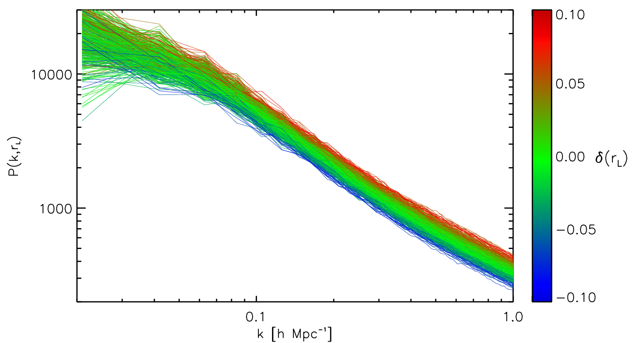
Refer to caption — Figure 1: Position-dependent power spectra measured from 512 subvolumes with $L=300~h^{-1}~{\rm Mpc}$ in one realization. The color represents $\bar{\delta}(\mathbf{r}_{L})$ of each subvolume.

Figure 1 shows the position-dependent power spectrum measured from 512 subvolumes with $L=300~h^{-1}~{\rm Mpc}$ in one realization. The color represents $\bar{\delta}(\mathbf{r}_{L})$ of each subvolume. The positive correlation between the subvolume power spectra and $\bar{\delta}(\mathbf{r}_{L})$ is obvious. The response $\tilde{f}(k)>0$ is clearly measurable at high significance in the simulations.

We measure the integrated bispectrum through

iB(k)=\frac{1}{N_{\rm cut}^{3}}\sum_{i=1}^{N_{\rm cut}^{3}}P(k,\mathbf{r}_{L,i})\bar{\delta}(\mathbf{r}_{L,i}),

(17)

where $P(k,\mathbf{r}_{L,i})$ and $\bar{\delta}(\mathbf{r}_{L,i})$ are measured in the $i^{\rm th}$ subvolume. Further, motivated by eq. (12), we normalize the integrated bispectrum by the mean power spectrum in the subvolumes, $\langle P(k,\mathbf{r}_{L})\rangle=N_{\rm cut}^{-3}\sum_{i=1}^{N_{\rm cut}^{3}}P(k,\mathbf{r}_{L,i})$ , and the variance of the mean density fluctuation in the subvolumes, $\langle\sigma_{L}^{2}\rangle=N_{\rm cut}^{-3}\sum_{i=1}^{N_{\rm cut}^{3}}\bar{\delta}^{2}(\mathbf{r}_{L,i})$ . This quantity, $iB(k)/[\langle P(k,\mathbf{r}_{L})\rangle\langle\sigma_{L}^{2}\rangle]$ , is the normalized integrated bispectrum we have defined at the end of section 2.3, and is equal to the linear response function, $d\ln P(k)/d\bar{\delta}$ , given in eq. (15) in the limit of $kL\to\infty$ .

Figure 2 shows the normalized integrated bispectrum, averaged over 160 collisionless $N$ -body simulations at different redshifts. For clarity, no error bars are shown in this figure. We have compared the results with a higher-resolution simulation with $1536^{3}$ particles and starting at higher redshift ( $z=49$ compared to $z=19$ for our 160 simulations). For the scales and redshifts shown in figure 2, the differences are less than 1%. However, we expect an up to 5% uncertainty in the integrated bispectrum at $z=3$ (less at lower $z$ ) due to transients which affect the bispectrum more strongly than the power spectrum [11], as well as other systematics such as mass resolution.

Since the initial conditions are Gaussian, the bispectrum is generated entirely by non-linear gravitational evolution. We thus measure the effect of a long-wavelength density perturbation on the evolution of small-scale structures. The wiggles visible in each panel of figure 2 are due to the BAOs. The BAOs in the right panel are strongly damped because the box size ( $120~h^{-1}~{\rm Mpc}$ ) approaches the BAO scale, and the window function smears the BAO feature [12]. Further, BAO amplitudes are larger at higher redshifts as they are less damped by non-linear evolution [13]. The broad-band shape of the normalized integrated bispectrum evolves on small scales due to non-linear evolution, leading to an effective steepening of its slope. We now turn to the theoretical modeling of the results shown in figure 2.

4 Theoretical modeling

We use two different approaches to model the integrated bispectrum. In the first approach, we model the bispectrum and compute the integral to obtain the integrated bispectrum. In the second approach, we model the response of the small-scale power spectrum to a long wavelength perturbation directly using the “separate universe” picture. For clarity, we will show the comparison between model prediction and simulations only for the $L=300~h^{-1}~{\rm Mpc}$ subvolumes ( $N_{\rm cut}=8$ ). The agreement with simulations is independent of subvolume size as long as the subvolume size is large enough for $\bar{\delta}$ to be in the linear regime, and the window function is taken into account.

4.1 Bispectrum modeling

We compute the integrated bispectrum by using a model for the bispectrum in eq. (8) and perform the eight-dimensional integral. Because of the high dimensionality, we use the Monte Carlo integration routine in GNU Scientific Library to evaluate the angular-averaged integrated bispectrum. In the following, we consider two different models for the matter bispectrum.

4.1.1 Standard perturbation theory

The standard perturbation theory (SPT) [1] gives the tree-level matter bispectrum as

B_{\rm SPT}(\mathbf{k}_{1},\mathbf{k}_{2},\mathbf{k}_{3})=2[P_{l}(k_{1})P_{l}(k_{2})F_{2}(\mathbf{k}_{1},\mathbf{k}_{2})+2\>\rm perm],

(18)

where $P_{l}(k)$ is the linear matter power spectrum, and

F_{2}(\mathbf{k}_{1},\mathbf{k}_{2})=\frac{5}{7}+\frac{1}{2}\frac{\mathbf{k}_{1}\cdot\mathbf{k}_{2}}{k_{1}k_{2}}\left(\frac{k_{1}}{k_{2}}+\frac{k_{2}}{k_{1}}\right)+\frac{2}{7}\left(\frac{\mathbf{k}_{1}\cdot\mathbf{k}_{2}}{k_{1}k_{2}}\right)^{2}~.

(19)

In order to normalize the integrated bispectrum, we need an expression for the mean subvolume power spectrum $\langle P_{L}\rangle$ . For this we use the linear power spectrum convolved with the window function,

\langle P_{L,l}(k)\rangle=\frac{1}{V_{L}}\int\frac{d^{3}q}{(2\pi)^{3}}~P_{l}(|\mathbf{k}-\mathbf{q}|)|W_{L}(\mathbf{q})|^{2}~,

(20)

while the variance of the mean density fluctuation in the subvolumes is given by eq. (13). Both quantities are calculated through Monte Carlo integration.

We compare the normalized integrated bispectrum measured from the simulations with the SPT prediction in figure 3 (red lines). The SPT prediction is independent of redshift. This is because the linear power spectra at various redshifts are only different by the wavenumber-independent linear growth factor, $D^{2}(z)$ . Therefore, the linear growth factor cancels out in the normalized integrated bispectrum. The SPT predictions agree with the simulations relatively well at $z\geq 1$ and $k\lesssim 0.2~h~{\rm Mpc}^{-1}$ , whereas they fail at lower redshifts as well as on smaller scales, where non-linearities become too strong to be described by SPT. Especially, the BAO amplitudes at $k\gtrsim 0.2~h~{\rm Mpc}^{-1}$ are affected: while the SPT predictions are redshift-independent, the simulations show smaller BAO amplitudes at lower redshifts.

The eight-dimensional integral in eq. (8) simplifies greatly if we focus on the squeezed-limit bispectrum. In appendix A, we show

			$\displaystyle\int\frac{d^{2}\Omega_{\hat{\mathbf{k}}}}{4\pi}~B_{\rm SPT}(\mathbf{k}-\mathbf{q}_{1},-\mathbf{k}+\mathbf{q}_{1}+\mathbf{q}_{3},-\mathbf{q}_{3})$		(21)
		$\displaystyle=$	$\displaystyle\left[\frac{68}{21}-\frac{1}{3}\frac{d\ln k^{3}P_{l}(k)}{d\ln k}\right]P_{l}(k)P_{l}(q_{3})+\mathcal{O}\left[\left(\frac{q_{1,3}}{k}\right)^{2}\right]~,$		(21)

for $k\gg q_{1},q_{3}$ . This result has the same form as given in eq. (11). We can then apply eq. (12) and perform all the integrals analytically in the limit of $kL\to\infty$ to obtain

$\displaystyle iB_{\rm SPT}(k)$	$\displaystyle=$	$\displaystyle\frac{1}{V_{L}^{2}}\int\frac{d^{2}\Omega_{\hat{\mathbf{k}}}}{4\pi}\int\frac{d^{3}q_{1}}{(2\pi)^{3}}\int\frac{d^{3}q_{3}}{(2\pi)^{3}}~B_{\rm SPT}(\mathbf{k}-\mathbf{q}_{1},-\mathbf{k}+\mathbf{q}_{1}+\mathbf{q}_{3},-\mathbf{q}_{3})$	(22)
		$\displaystyle\hskip 136.5733pt\times W_{L}(\mathbf{q}_{1})W_{L}(-\mathbf{q}_{1}-\mathbf{q}_{3})W_{L}(\mathbf{q}_{3})$
	$\displaystyle\stackrel{{\scriptstyle kL\to\infty}}{{=}}$	$\displaystyle\left[\frac{68}{21}-\frac{1}{3}\frac{d\ln k^{3}P_{l}(k)}{d\ln k}\right]P_{l}(k)\sigma_{L}^{2}~.$

Comparing this result with eq. (15), we find that the linear response of the power spectrum in SPT is given by

\left.\frac{d\ln P_{l}(k)}{d\bar{\delta}}\right|_{\rm SPT}=\frac{68}{21}-\frac{1}{3}\frac{d\ln k^{3}P_{l}(k)}{d\ln k}.

(23)

The green lines in figure 3 show the squeezed-limit approximation given in eq. (22). While they are different from the full integration (red lines) at $k\lesssim 0.2~h~{\rm Mpc}^{-1}$ , for which the squeezed-limit approximation fails and the direct integration is required, they agree well—with the fractional difference being less than 1.5% (1% for $L=600\,h^{-1}$ Mpc)—at $k\gtrsim 0.2~h~{\rm Mpc}^{-1}$ , corresponding to a value of $1/(kL)\lesssim 0.02$ . Thus, the squeezed-limit is reached already with good precision for $kL\gtrsim 50$ .

Eq. (22) does not contain any window function effect apart from that in the variance $\sigma_{L}^{2}$ . While this is a good approximation for the slowly-varying part of the integrated bispectrum, it does not capture the smearing of the BAO features due to the window function. We incorporate this effect by replacing $d\ln P_{l}(k)/d\ln k$ with appropriately convolved forms, ${\rm conv}[dP_{l}(k)/d\ln k]\>/\>{\rm conv}[P_{l}(k)]$ , in eq. (22). This form is motivated by the separate universe approach discussed in section 4.2, and provides an accurate result as shown in figure 3.

4.1.2 Bispectrum fitting formula

The SPT predictions fail on smaller scales as well as at lower redshifts where non-linearity becomes too strong to be described by SPT. An empirical fitting formula for non-linear evolution of the matter bispectrum was proposed in [14] and further improved in [15]. In short, the form is the same as the tree-level matter bispectrum, but $F_{2}(\mathbf{k}_{1},\mathbf{k}_{2})$ is replaced by an effective kernel, $F_{2}^{\rm eff}(\mathbf{k}_{1},\mathbf{k}_{2})$ , which contains nine fitting parameters, $\{a_{1},\cdots a_{9}\}$ , to account for non-linearity (see eqs. 2.6 and 2.12 in [15] for details). Therefore, we use $F_{2}^{\rm eff}(\mathbf{k}_{1},\mathbf{k}_{2})$ and compute the integrated bispectrum by performing the eight-dimensional integral numerically with Monte Carlo integration. We use the same values of the best-fit parameters provided in table 2 of [15], which were calibrated by fitting to simulation results between $z=0$ and $z=1.5$ . In contrast to the SPT formalism that uses the linear power spectrum in eq. (18), the fitting formula uses the non-linear power spectrum, for which we use the mean power spectrum measured from the 160 simulation boxes. For the normalization of the integrated bispectrum, we convolve the non-linear power spectrum with the subvolume window function as in eq. (20). Note that the $F_{2}^{\rm eff}$ fitting formula is not specifically designed for the squeezed configuration, but instead was calibrated to a wide range of triangle configurations of the matter bispectrum.

The blue lines in figure 3 show the normalized integrated bispectrum computed with $F_{2}^{\rm eff}$ , which clearly depends on redshift. At $z\gtrsim 1$ , the $F_{2}^{\rm eff}$ modeling and the simulations are in good agreement at $k\lesssim 0.2~h~{\rm Mpc}^{-1}$ . At $k>0.2~h~{\rm Mpc}^{-1}$ , although the $F_{2}^{\rm eff}$ modeling predicts larger broad-band power of the normalized integrated bispectrum, the BAO amplitudes still agree well with the simulations. This is most obvious for the two BAO peaks at $0.25~h~{\rm Mpc}^{-1}\leq k\leq 0.35~h~{\rm Mpc}^{-1}$ . On the other hand, at $z=0$ , the $F_{2}^{\rm eff}$ modeling predicts much larger normalized integrated bispectrum on small scales than measured in the simulations, so that the fitting formula does not perform much better than tree-level perturbation theory at $z=0$ .

4.2 Separate universe approach

In the second approach, we compute the effects of a long-wavelength density fluctuation on the small-scale power spectrum by treating each over- and under dense region as a separate universe with a different background density. This approach thus neglects the finite size of the subvolumes and is valid for wavenumbers which satisfy $kL\gg 1$ (specifically, $kL\gtrsim 50$ for percent-level accuracy).

The power spectrum in a separate universe with an infinite-wavelength density perturbation, $\bar{\delta}$ , with respect to the global flat $\Lambda$ CDM cosmology can be expanded as in eq. (14). Through eq. (15), the normalized integrated bispectrum is equal to the linear response of the non-linear matter power spectrum at wavenumber $k$ to $\bar{\delta}$ :

\frac{iB(k)}{P(k)\sigma_{L}^{2}}=\frac{d\ln P(k)}{d\bar{\delta}}\,.

(24)

This is not exactly true if the subvolumes for which $iB(k)$ is measured are not spherical. For example, since the cubic window function is anisotropic, the integrated bispectrum might pick up contributions from the tidal field. However, we have verified that the anisotropy of the cubic window function has a negligible effect, by computing the dipole and quadrupole of the integrated bispectrum through eq. (8). The ratios to the monopole are less than $10^{-5}$ on the scales of interest.

A universe with an infinite-wavelength density perturbation with respect to a flat fiducial cosmology is equivalent to a universe with non-zero curvature (e.g., [16]). This alters the scale factor-time relation, Hubble rate, and linear growth, and thus affects the power spectrum. Recent papers [17, 18, 19, 20] have studied this topic. We briefly summarize the result here. We write the fractional mass density perturbation with respect to the fiducial flat universe as

\bar{\delta}(t)=\frac{\tilde{\bar{\rho}}(t)}{\bar{\rho}(t)}-1=\frac{D(t)}{D(t_{0})}\bar{\delta}_{0}\,,

(25)

where $\bar{\rho}(t)$ is the background matter density in the fiducial flat cosmology, $D(t)$ is the linear growth factor in the same cosmology, $\tilde{\bar{\rho}}$ is the background matter density in a slightly curved universe, $t_{0}$ is a reference time, and $\bar{\delta}_{0}$ is the density perturbation at $t_{0}$ . In the following, $t_{0}$ will stand for the present epoch and we choose $a(t_{0})=1$ . Quantities in the modified (curved) cosmology are denoted with a tilde, such as $\tilde{a}(t)$ for the modified scale factor-time relation. Note that the time coordinates are the same in both cosmologies in the sense that they are the proper time for comoving observers in the absence of perturbations. For a fiducial flat $\Lambda$ CDM cosmology, the modified curved cosmology to linear order in $\bar{\delta}$ is described by modified cosmological parameters (also see [21, 20])

$\displaystyle\tilde{H}_{0}=\>$	$\displaystyle H_{0}\left(1+\delta_{H}\right)$
$\displaystyle\tilde{\Omega}_{m}=\>$	$\displaystyle\Omega_{m}\left(1-2\delta_{H}\right)$
$\displaystyle\tilde{\Omega}_{K}=\>$	$\displaystyle-\left(\Omega_{m}+\frac{2}{3}f_{0}\right)\bar{\delta}_{0}$
$\displaystyle\tilde{\Omega}_{\Lambda}=\>$	$\displaystyle\Omega_{\Lambda}\left(1-2\delta_{H}\right)\,,$	(26)

where

\delta_{H}\equiv\left(-\frac{1}{2}\Omega_{m}-\frac{1}{3}f_{0}\right)\bar{\delta}_{0},

(27)

and $f_{0}=f(t_{0})$ is the logarithmic growth rate evaluated at $t_{0}$ . The scale factor-time relation in the modified cosmology is given by

\tilde{a}(t)=a(t)\left[1-\frac{1}{3}\bar{\delta}(t)\right]\,.

(28)

Hence, observables calculated with respect to comoving coordinates in the modified cosmology $\tilde{a}(t)$ have to be transformed according to a coordinate rescaling of

\mathbf{x}\to\mathbf{x}^{\prime}=\mathbf{x}\left[1-\frac{1}{3}\bar{\delta}(t)\right]\,.

(29)

For the power spectrum, this corresponds to (see appendix A of [22])

P(k,t)\to P(k,t)\left[1-\frac{1}{3}\frac{d\ln k^{3}P(k,t)}{d\ln k}\bar{\delta}(t)\right]\,.

(30)

Let us denote the power spectrum in the modified cosmology described by eq. (26) as $\tilde{P}(\tilde{k},t)$ . This power spectrum refers to the modified mean density, which is given by the fiducial mean density multiplied by $1+\bar{\delta}(t)$ . We then have for the power spectrum with respect to the fiducial mean density

P(\tilde{k},t)=\left[1+2\bar{\delta}(t)\right]\tilde{P}(\tilde{k},t)\,.

(31)

Converting $\tilde{k}$ to $k$ with eq. (30) and using the scale factor instead of time, the power spectrum in the presence of $\bar{\delta}$ is given by

P(k,a|\bar{\delta})=\tilde{P}\left(k,a\left[1-\frac{1}{3}\bar{\delta}(a)\right]\right)\left[1+\left(2-\frac{1}{3}\frac{d\ln k^{3}P(k,a)}{d\ln k}\right)\bar{\delta}(a)\right]~.

(32)

Note that this expression is only valid to linear order in $\bar{\delta}$ .

Both $P(k)$ and $\bar{\delta}$ are measured in a finite volume, described by the window function $W_{L}$ . In order to take this into account, eq. (32) is convolved by the window function. Note that we take the convolution after applying the derivative $d\ln k^{3}P(k)/d\ln k$ , rather than taking the derivative of the convolved power spectrum. This is because the window function is fixed in terms of observed coordinates (in the fiducial cosmology), i.e., it is not subject to the rescaling of eq. (29). Taking the slope of the convolved power spectrum would correspond to a window function defined in the “local” curved cosmology.

4.2.1 Linear power spectrum

For the linear power spectrum, $P_{l}$ , we have

\tilde{P}_{l}\left(k,a\left[1-\frac{1}{3}\bar{\delta}(a)\right]\right)=\left(\frac{\tilde{D}\left(a\left[1-\frac{1}{3}\bar{\delta}(a)\right]\right)}{D(a)}\right)^{2}P_{l}(k,a)\,.

(33)

The linear growth factor is changed following (see appendix D in [16])

\tilde{D}\left(a\left[1-\frac{1}{3}\bar{\delta}(a)\right]\right)=D(a)\left[1+\frac{13}{21}\bar{\delta}(a)\right]\,,

(34)

where $D(a)$ is the growth factor in the fiducial cosmology. The prefactor $13/21$ is only strictly valid for an Einstein-de Sitter cosmology; however, the cosmology dependence is very mild. The fractional difference of $d\ln D(a)/d\bar{\delta}$ between $\Lambda$ CDM cosmology and Einstein-de Sitter universe at $z=0$ is at the 0.1% level.

Putting everything together, eq. (32) yields for the linear response function of the linear power spectrum

\frac{d\ln P_{l}(k,a)}{d\bar{\delta}(a)}=\frac{68}{21}-\frac{1}{3}\frac{d\ln k^{3}P_{l}(k,a)}{d\ln k}\,.

(35)

This result (which again is only exact for Einstein-de Sitter) matches the expression derived from the $F_{2}$ kernel given in eq. (23).

4.2.2 SPT 1-loop power spectrum

Expanding matter density fluctuations to third order, one obtains the so-called “SPT 1-loop power spectrum” given by $P(k,a)=P_{l}(k,a)+P_{22}(k,a)+2P_{13}(k,a)$ , where [1]

$\displaystyle P_{22}(k,a)$	$\displaystyle=$	$\displaystyle 2\int\frac{d^{3}q}{(2\pi)^{3}}P_{l}(q,a)P_{l}(\|\mathbf{k}-\mathbf{q}\|,a)\left[F_{2}(\mathbf{q},\mathbf{k}-\mathbf{q})\right]^{2},$	(36)
$\displaystyle 2P_{13}(k,a)$	$\displaystyle=$	$\displaystyle\frac{2\pi k^{2}}{252}P_{l}(k,a)\int_{0}^{\infty}\frac{dq}{(2\pi)^{3}}P_{l}(q,a)$
		$\displaystyle\times\Biggl[100\frac{q^{2}}{k^{2}}-158+12\frac{k^{2}}{q^{2}}-42\frac{q^{4}}{k^{4}}+\frac{3}{k^{5}q^{3}}(q^{2}-k^{2})^{3}(2k^{2}+7q^{2})\ln\left(\frac{k+q}{\|k-q\|}\right)\Biggl].$

Both $P_{22}$ and $P_{13}$ are proportional to $D^{4}(a)$ . Modifying the growth factor as described in section 4.2.1, we obtain the linear response function of the SPT 1-loop power spectrum as

\frac{d\ln P(k,a)}{d\bar{\delta}(a)}=\frac{68}{21}-\frac{1}{3}\frac{d\ln k^{3}P(k,a)}{d\ln k}+\frac{26}{21}\frac{P_{22}(k,a)+2P_{13}(k,a)}{P(k,a)}\,.

(37)

Note that this can easily be generalized to $n$ loops in perturbation theory by using that $d\ln P_{(n-{\rm loop})}(k,a)/d\ln D(a)=2n+2$ . We include the window function effect by computing ${\rm conv}[dP(k)/d\bar{\delta}]/{\rm conv}[P(k)]$ .

Figure 4 compares the linear theory and the SPT 1-loop predictions with the $N$ -body simulation results. The SPT 1-loop prediction captures the damping of BAOs due to non-linear evolution, and agrees well with the simulation results at $z=1$ , 2, and 3. This is expected from the excellent performance of the 1-loop matter power spectrum at high redshifts as demonstrated by [23]. The agreement degrades rapidly at $z=0$ , also as expected. Note that comparing $z=2$ and 3, the 1-loop prediction seems to agree better with the measurements at $z=2$ . However, as mentioned in section 3, transients and other systematics might have an impact of up to 5% on the measurements at $z=3$ , which is larger than the difference shown in the top left panel of figure 4.

4.2.3 halofit and Coyote emulator

We now apply the separate universe approach to simulation-calibrated fitting formulae for the non-linear matter power spectrum, specifically the halofit prescription [24] and the Coyote emulator [25]. These prescriptions yield $\tilde{P}(k,a)$ for a given set of cosmological parameters, so that eq. (32) can be immediately applied. However, the Coyote emulator does not provide predictions for curved cosmologies, and we hence adopt a simpler approach here.

In case of the linear power spectrum, the effect of the modified cosmology enters only through the modified growth factor given in eq. (34). Correspondingly, we can approximate the effect on the non-linear power spectrum by a change in the value of the power spectrum normalization $\sigma_{8}$ at redshift zero,

\sigma_{8}\to\left[1+\frac{13}{21}\bar{\delta}_{0}\right]\sigma_{8}~,

(38)

where we have used the Einstein-de Sitter prediction. Therefore, the non-linear power spectrum response becomes

\frac{d\ln P_{nl}(k,a)}{d\bar{\delta}(a)}=\frac{13}{21}\frac{d\ln P_{nl}(k,a)}{d\ln\sigma_{8}}+2-\frac{1}{3}\frac{d\ln k^{3}P_{nl}(k,a)}{d\ln k}~.

(39)

The results of applying eq. (39) to halofit (red) and the Coyote emulator (green) are shown in figure 5. In terms of broad-band power, the halofit prediction provides a good match. However, the predicted BAO amplitude are larger than the measurement, especially at low redshift at $k\gtrsim 0.3~h~{\rm Mpc}^{-1}$ . Also, while the BAO phases of halofit follow the SPT prediction, there are some differences with respect to the measurement of the $N$ -body simulations due to the non-linear evolution. The Coyote emulator performs to better than $\sim 2$ % over the entire range of scales and redshifts. It slightly underpredicts the small-scale power at $k>0.3~h~{\rm Mpc}^{-1}$ for $z\geq 1$ . For redshifts $z\geq 2$ and on the scales considered, the 1-loop predictions are of comparable accuracy to the Coyote emulator, while the latter provides a better fit at lower redshifts. Finally, note also our previous caveat regarding transients at the end of section 4.2.2.

4.2.4 Halo model

In the halo model (see [26] for a review), all matter is assumed to be contained within halos with a certain distribution of mass given by the mass function, and a certain density profile. Along with the clustering properties of the halos, these quantities then determine the statistics of the matter density field on all scales including the non-linear regime. $N$ -point functions can be conveniently decomposed into 1- through $N$ -halo pieces. In the following, we will follow the most common halo model approach and assume a linear local bias of the halos.

Adopting the notation of [27], the halo model power spectrum, $P_{\rm HM}(k)$ , is given by

$\displaystyle P_{\rm HM}(k)=\>$	$\displaystyle P^{\rm 2h}(k)+P^{\rm 1h}(k)$	(40)
$\displaystyle P^{\rm 2h}(k)=\>$	$\displaystyle\left[I^{1}_{1}(k)\right]^{2}P_{l}(k)$
$\displaystyle P^{\rm 1h}(k)=\>$	$\displaystyle I^{0}_{2}(k,k)\,,$

where

I^{n}_{m}(k_{1},\cdots k_{m})\equiv\int d\ln M\>n(\ln M)\left(\frac{M}{\bar{\rho}}\right)^{m}\,b_{n}(M)\,u(M|k_{1})\cdots u(M|k_{m})\,,

(41)

and $n(\ln M)$ is the mass function (comoving number density per interval in log mass), $M$ is the halo mass, $b_{n}(M)$ is the $n$ -th order local bias parameter, and $u(M|k)$ is the dimensionless Fourier transform of the halo density profile, for which we use the NFW profile [28]. We normalize $u$ so that $u(M|k\to 0)=1$ . The notation given in eq. (41) assumes $b_{0}\equiv 1$ . $u(M|k)$ depends on $M$ through the scale radius $r_{s}$ , which in turn is given through the mass-concentration relation. All functions of $M$ in eq. (41) are also functions of $z$ although we have not shown this for clarity. In the following, we adopt the Sheth-Tormen mass function [29] with the corresponding peak-background split bias, and the mass-concentration relation of [30]. The exact choice of the latter has negligible impact on the mildly non-linear scales considered in this paper.

We now derive how the power spectrum given in eq. (40) responds to an infinitely long-wavelength density perturbation $\bar{\delta}$ , as was done for the halofit and Coyote emulator approaches. For this, we consider the 1-halo and 2-halo terms separately. The key physical assumption we make is that halo profiles in physical coordinates are unchanged by the long-wavelength density perturbation. That is, halos at a given mass $M$ in the presence of $\bar{\delta}$ have the same scale radius $r_{s}$ and scale density $\rho(r_{s})$ as in the fiducial cosmology. This assumption, which is related to the stable clustering hypothesis, can be tested independently with simulations, but this goes beyond the scope of this paper. Given this assumption, the density perturbation $\bar{\delta}$ then mainly affects the linear power spectrum, which determines the halo-halo clustering (2-halo term), and the abundance of halos at a given mass.

We begin with the 2-halo term. The response of the linear power spectrum is given by eq. (35). The expression for the 2-halo term in eq. (40) is simply the convolution (in real space) of the halo correlation function in the linear bias model with the halo density profiles. By assumption, the density profiles do not change, hence $I^{1}_{1}$ only changes through the bias $b_{1}(M)$ and the mass function $n(\ln M)$ . The bias $b_{N}(M)$ quantifies the $N$ -th order response of the mass function $n(\ln M)$ to an infinite-wavelength density perturbation [31, 32]:

b_{N}(M)=\frac{1}{n(\ln M)}\frac{\partial^{N}n(\ln M)}{\partial\bar{\delta}^{N}}\Big|_{0}\,,

(42)

We then have

	$\displaystyle\frac{\partial n(\ln M)}{\partial\bar{\delta}}\Big\|_{0}=\>$	$\displaystyle b_{1}(M)n(\ln M)\,,$
	$\displaystyle\frac{\partial b_{1}(M)}{\partial\bar{\delta}}\Big\|_{0}=\>$	$\displaystyle-[b_{1}(M)]^{2}+b_{2}(M)\,.$		(43)

Thus,

$\displaystyle\frac{\partial}{\partial\bar{\delta}}I^{1}_{1}(k)=\>$	$\displaystyle\int d\ln M\>n(\ln M)\left(\frac{M}{\bar{\rho}}\right)\left([b_{1}(M)]^{2}-[b_{1}(M)]^{2}+b_{2}(M)\right)u(M\|k)$
$\displaystyle=\>$	$\displaystyle\int d\ln M\>n(\ln M)\left(\frac{M}{\bar{\rho}}\right)b_{2}(M)u(M\|k)$
$\displaystyle=\>$	$\displaystyle I^{2}_{1}(k)\,.$	(44)

In the large-scale limit, $k\to 0$ , this vanishes by way of the halo model consistency relation

\int d\ln M\>n(\ln M)\left(\frac{M}{\bar{\rho}}\right)b_{N}(M)=\left\{\begin{array}[]{ll}1,&N=1\,,\\ 0,&N\geq 1\,.\end{array}\right.

(45)

For finite $k$ however, eq. (44) does not vanish. Thus, the linear response function of the two-halo term becomes

\frac{dP^{\rm 2h}(k)}{d\bar{\delta}}\Big|_{0}=\left[\frac{68}{21}-\frac{1}{3}\frac{d\ln k^{3}P_{l}(k)}{d\ln k}\right]P^{\rm 2h}(k)+2I^{2}_{1}(k)I^{1}_{1}(k)P_{l}(k)\,.

(46)

Note that we recover the tree-level result given in eq. (35) in the large-scale limit. Strictly speaking, this expression is not consistent, since the term $I^{2}_{1}$ implies a non-zero $b_{2}$ while in eq. (40) we have assumed a pure linear bias. Of course, if we allowed for $b_{2}$ in eq. (40), we would obtain a contribution from $b_{3}$ in eq. (46), and so on. This reflects the fact that the halo model itself cannot be made entirely self-consistent. Note that in eq. (46) the slope is taken from the linear, not 2-halo power spectrum. This is a consequence of our assumption that halo profiles do not change due to $\bar{\delta}$ ; in other words, having $d\ln k^{3}P^{\rm 2h}/d\ln k$ would imply that the profiles do change (in the sense that they are fixed in comoving, rather than physical coordinates).

We now turn to the one-halo term. Given our assumption about density profiles, this term is much simpler. The only effect is the change in the mass function, which through eq. (42) (for $N=1$ ) yields

\frac{\partial}{\partial\bar{\delta}}I^{0}_{2}(k,k)=I^{1}_{2}(k,k)\,.

(47)

We thus obtain

\displaystyle\frac{dP^{\rm 1h}(k)}{d\bar{\delta}}\Big|_{0}=\>

\displaystyle I^{1}_{2}(k,k)\,.

(48)

Putting everything together, we obtain

\frac{d\ln P_{\rm HM}(k)}{d\bar{\delta}}\Big|_{0}=\left[P_{\rm HM}(k)\right]^{-1}\left[\left(\frac{68}{21}-\frac{1}{3}\frac{d\ln k^{3}P_{l}(k)}{d\ln k}\right)P^{\rm 2h}(k)+2I^{2}_{1}(k)I^{1}_{1}(k)P_{l}(k)+I^{1}_{2}(k,k)\right]\,.

(49)

The prediction of eq. (49) is shown as the blue lines in figure 5. The amplitude and broad-band shape agree with the simulations well. The main discrepancy in the halo model prediction is the insufficient damping of the BAO wiggles.

An alternative approach to derive the halo model prediction for $iB(k)$ is to use higher $N$ -point functions [19, 20], which are decomposed into $1-,\dots,N-$ halo terms. We now compare eq. (49) with the results of [20], which were derived from the halo model four-point function in the collapsed limit. Note that the squeezed limit is assumed in both approaches. Their eq. (27) is

\frac{d\ln P_{\rm HM}(k)}{d\bar{\delta}}\Big|_{0}=\left[P_{\rm HM}(k)\right]^{-1}\left[\left(\frac{68}{21}-\frac{1}{3}\frac{d\ln k^{3}P^{\rm 2h}(k)}{d\ln k}\right)P^{\rm 2h}(k)+I^{1}_{2}(k,k)\right]\,.

(50)

There are two differences to eq. (49): the term $\propto I^{2}_{1}$ is absent, and the slope is taken from from $P^{\rm 2h}$ rather than $P_{l}$ . The $I^{2}_{1}$ term is absent in eq. (50) as by assumption $b_{2}$ was taken to be zero in the four-point function of [20]; as discussed above, its inclusion is somewhat ambiguous given the lack of self-consistency of the halo model approach. The different power spectrum slopes are due to the different sources of this term in the two derivations. In our case, the assumption of unchanged halo profiles dictates the form of eq. (49). In the derivation of eq. (50), the slope originates from the integral over the $F_{2}$ kernel in the 3-halo term, which proceeds as described in appendix A but involves $P^{\rm 2h}$ instead of $P_{l}$ . Note however that the numerical difference between eq. (50) and eq. (49) is only at the percent level.

4.3 Dependence on cosmological parameters

Both the matter power spectrum and (integrated) bispectrum depend on the cosmological parameters such as $\Omega_{m},\,\sigma_{8},n_{s}$ . However, the normalized integrated bispectrum is much less sensitive to cosmology as the leading cosmology dependence is taken out by the normalizing denominator.

Eq. (37) is useful for understanding the dependence of the response function of the power spectrum (and thus the normalized integrated bispectrum) on cosmological parameters. The second term depends on the local spectral index of the matter power spectrum, $d\ln k^{3}P(k)/d\ln k$ , which depends on the initial power spectrum tilt, $n_{s}$ , and the matter and radiation densities which change the redshift of matter-radiation equality as well as the BAO scale. It also depends on the shape of BAO wiggles, and increasing the amplitude of the matter power spectrum ( $\sigma_{8}$ ) leads to a stronger damping of the BAO feature. Increasing $\sigma_{8}$ further increases the last term, which is proportional to $\sigma_{8}^{2}$ .

Figure 6 shows the linear response functions, $d\ln P(k,a)/d\bar{\delta}(a)$ computed from the SPT 1-loop power spectrum (eq. (37)) at $z=2$ when varying cosmological parameters by $\pm 5\%$ . The effects on the response functions are at the percent level or less, illustrating the weak cosmology dependence of this observable. On the scales considered, the shift in the BAO scale when varying $\Omega_{m}$ leads to the relatively largest effect. We expect that the sensitivity to changes in $\sigma_{8}$ will be higher on smaller, more nonlinear scales.

5 Conclusions

In this paper, we have proposed a novel method to measure the squeezed-limit bispectrum. By correlating the mean density fluctuation and the position-dependent power spectrum, we obtain a measurement of a certain moment of the bispectrum (integrated bispectrum) without having to actually measure three-point correlations in the data. The integrated bispectrum is dominated by the squeezed-limit bispectrum, which is much easier to model than the full bispectrum for all configurations. This is evidenced by figures 4–5, where we show model predictions accurate to a few percent using existing techniques and without tuning any parameters.

A further, key advantage of this new observable is that both the mean density fluctuation and the power spectrum are significantly easier to measure in actual surveys than the bispectrum in terms of survey selection functions. In particular, the procedures developed for power spectrum estimation can be directly applied to the measurement of the position-dependent power spectrum. Additionally, the position-dependent power spectrum depends on only one wavenumber (at fixed size of the subvolume) rather than the three wavenumbers of the bispectrum. Consequently, the covariance matrix also becomes easier to model.

We have measured the position-dependent power spectrum in 160 collisionless $N$ -body simulations with Gaussian initial conditions, and have used two different approaches — bispectrum modeling and the separate universe approach — to model the measurements. All of the approaches work well on large scales, $k\lesssim 0.2~h\,{\rm Mpc}^{-1}$ , and at high redshift. On small scales, where non-linearities become important, the separate universe approach (section 4.2) applied through the Coyote emulator prescription performs best at redshifts $z<2$ , while the SPT 1-loop predictions perform equally well at $z\geq 2$ . Both show agreement to within a few percent up to $k=0.4~h\,{\rm Mpc}^{-1}$ . Accurate predictions for the position-dependent power spectrum on these and even smaller scales can be obtained by applying the separate universe approach to dedicated small-box $N$ -body simulations of curved cosmologies [20]. We shall study this in an upcoming paper.

The normalized integrated bispectrum is relatively insensitive to changes in cosmological parameters (section 4.3), and we do not expect that it will allow for competitive cosmology constraints. On the other hand, this property can also be an advantage: since this observable can be predicted accurately without requiring a precise knowledge of the cosmology, it can serve as a useful systematics test for example in weak lensing surveys. As an example, consider eq. (12) applied to shear measurements. A constant multiplicative bias $1+m$ in the shear estimation contributes a factor $(1+m)^{3}$ on the left hand side of the equation, and a factor $(1+m)^{4}$ on the right hand side. Thus, by comparing the measured normalized integrated bispectrum with the (essentially cosmology-independent) expectation, one can constrain the multiplicative shear bias.

The position-dependent power spectrum can also naturally be applied to the case of spectroscopic galaxy surveys, in which case the non-linear bias of the observed tracers also contributes to the bispectrum and position-dependent power spectrum. Thus, when applied to halos or galaxies, this observable can serve as an independent probe of the bias parameters and break degeneracies between bias and growth which are present when only considering the halo or galaxy power spectrum. We shall apply this new method to halos in $N$ -body simulations, as well as to data from galaxy surveys in future papers. Finally, this approach can also be immediately applied to the projected matter density distribution as measured through weak lensing. In this case, the complexities of bias are absent and the modeling we have presented in this paper should be sufficient to describe the measurements.

Acknowledgements.

We would like to thank Wayne Hu, Masahiro Takada, Simon White, and Donghui Jeong for useful discussions.

Appendix A Tree-level matter bispectrum in the squeezed configurations

In this appendix, we derive the squeezed-limit result eq. (21). The tree-level perturbation theory gives the matter bispectrum (with our notation)

$\displaystyle B(\mathbf{k}-\mathbf{q}_{1},-\mathbf{k}+\mathbf{q}_{1}+\mathbf{q}_{3},-\mathbf{q}_{3})$	$\displaystyle=$	$\displaystyle 2[F_{2}(\mathbf{k}-\mathbf{q}_{1},-\mathbf{k}+\mathbf{q}_{1}+\mathbf{q}_{3})P(\|\mathbf{k}-\mathbf{q}_{1}\|)P(\|-\mathbf{k}+\mathbf{q}_{1}+\mathbf{q}_{3}\|)$	(51)
		$\displaystyle+F_{2}(\mathbf{k}-\mathbf{q}_{1},-\mathbf{q}_{3})P(\|\mathbf{k}-\mathbf{q}_{1}\|)P(q_{3})$
		$\displaystyle+F_{2}(-\mathbf{k}+\mathbf{q}_{1}+\mathbf{q}_{3},-\mathbf{q}_{3})P(\|-\mathbf{k}+\mathbf{q}_{1}+\mathbf{q}_{3}\|)P(q_{3})]~,$

where $F_{2}(\mathbf{k}_{1},\mathbf{k}_{2})$ is

F_{2}(\mathbf{k}_{1},\mathbf{k}_{2})=\frac{5}{7}+\frac{1}{2}\frac{\mathbf{k}_{1}\cdot\mathbf{k}_{2}}{k_{1}k_{2}}\left(\frac{k_{1}}{k_{2}}+\frac{k_{2}}{k_{1}}\right)+\frac{2}{7}\left(\frac{\mathbf{k}_{1}\cdot\mathbf{k}_{2}}{k_{1}k_{2}}\right)^{2}~.

(52)

In the squeezed configurations, where $k\gg q_{1},q_{3}$ , we Taylor expand the power spectra and $F_{2}$ ’s. In the calculation, we keep terms to first order, e.g., keeping 1 and $q/k$ (ignoring $(q/k)^{n}$ for $n\geq 2$ ) or keeping $q/k$ and $(q/k)^{2}$ (ignoring $(q/k)^{n}$ for $n\geq 3$ ), and then combine them to see the leading order effect of the final result.

First, the amplitudes of the vectors can be calculated as

	$\displaystyle\|\mathbf{k}-\mathbf{q}_{1}\|$	$\displaystyle=$	$\displaystyle\sqrt{k^{2}+q_{1}^{2}-2\mathbf{k}\cdot\mathbf{q}_{1}}\approx k\left(1-\frac{\mathbf{k}\cdot\mathbf{q}_{1}}{k^{2}}\right)$
	$\displaystyle\|-\mathbf{k}+\mathbf{q}_{1}+\mathbf{q}_{3}\|$	$\displaystyle\approx$	$\displaystyle k\left[1-\frac{\mathbf{k}\cdot(\mathbf{q}_{1}+\mathbf{q}_{3})}{k^{2}}\right]~.$		(53)

Therefore, the power spectra are

	$\displaystyle P(\|\mathbf{k}-\mathbf{q}_{1}\|)$	$\displaystyle\approx$	$\displaystyle P\left(k-\frac{\mathbf{k}\cdot\mathbf{q}_{1}}{k}\right)\approx P(k)-\frac{\mathbf{k}\cdot\mathbf{q}_{1}}{k}\frac{dP(k)}{dk}=P(k)\left[1-\frac{\mathbf{k}\cdot\mathbf{q}_{1}}{k^{2}}\frac{d\ln P(k)}{d\ln k}\right]$
	$\displaystyle P(\|-\mathbf{k}+\mathbf{q}_{1}+\mathbf{q}_{3}\|)$	$\displaystyle\approx$	$\displaystyle P(k)\left[1-\frac{\mathbf{k}\cdot(\mathbf{q}_{1}+\mathbf{q}_{3})}{k^{2}}\frac{d\ln P(k)}{d\ln k}\right]~.$		(54)

The cosines between the vectors forming the squeezed triangle are

$\displaystyle\frac{(\mathbf{k}-\mathbf{q}_{1})\cdot(-\mathbf{k}+\mathbf{q}_{1}+\mathbf{q}_{3})}{\|\mathbf{k}-\mathbf{q}_{1}\|\|-\mathbf{k}+\mathbf{q}_{1}+\mathbf{q}_{3}\|}$	$\displaystyle\approx$	$\displaystyle[-k^{2}+\mathbf{k}\cdot(2\mathbf{q}_{1}+\mathbf{q}_{3})]\frac{1}{k^{2}}\left[1+\frac{\mathbf{k}\cdot\mathbf{q}_{1}}{k^{2}}\right]\left[1+\frac{\mathbf{k}\cdot(\mathbf{q}_{1}+\mathbf{q}_{3})}{k^{2}}\right]\approx-1$
$\displaystyle\frac{(\mathbf{k}-\mathbf{q}_{1})\cdot(-\mathbf{q}_{3})}{\|\mathbf{k}-\mathbf{q}_{1}\|\|-\mathbf{q}_{3}\|}$	$\displaystyle\approx$	$\displaystyle\frac{1}{kq_{3}}\left[-\mathbf{k}\cdot\mathbf{q}_{3}-\frac{(\mathbf{k}\cdot\mathbf{q}_{1})(\mathbf{k}\cdot\mathbf{q}_{3})}{k^{2}}+\mathbf{q}_{1}\cdot\mathbf{q}_{3}\right]$
$\displaystyle\frac{(-\mathbf{k}+\mathbf{q}_{1}+\mathbf{q}_{3})\cdot{-\mathbf{q}_{3}}}{\|-\mathbf{k}+\mathbf{q}_{1}+\mathbf{q}_{3}\|\|-\mathbf{q}_{3}\|}$	$\displaystyle\approx$	$\displaystyle\frac{1}{kq_{3}}\left[\mathbf{k}\cdot\mathbf{q}_{3}+\frac{(\mathbf{k}\cdot\mathbf{q}_{3})[(\mathbf{k}\cdot(\mathbf{q}_{1}+\mathbf{q}_{3})]}{k^{2}}-\mathbf{q}_{3}\cdot(\mathbf{q}_{1}+\mathbf{q}_{3})\right]~,$	(55)

the terms $k_{1}/k_{2}+k_{2}/k_{1}$ are

$\displaystyle\frac{\|\mathbf{k}-\mathbf{q}_{1}\|}{\|-\mathbf{k}+\mathbf{q}_{1}+\mathbf{q}_{3}\|}+\frac{\|-\mathbf{k}+\mathbf{q}_{1}+\mathbf{q}_{3}\|}{\|\mathbf{k}-\mathbf{q}_{1}\|}$	$\displaystyle\approx$	$\displaystyle 2$
$\displaystyle\frac{\|\mathbf{k}-\mathbf{q}_{1}\|}{\|-\mathbf{q}_{3}\|}+\frac{\|-\mathbf{q}_{3}\|}{\|\mathbf{k}-\mathbf{q}_{1}\|}$	$\displaystyle\approx$	$\displaystyle\frac{k}{q_{3}}\left[1-\frac{\mathbf{k}\cdot\mathbf{q}_{1}}{k^{2}}\right]$
$\displaystyle\frac{\|-\mathbf{k}+\mathbf{q}_{1}+\mathbf{q}_{3}\|}{\|-\mathbf{q}_{3}\|}+\frac{\|-\mathbf{q}_{3}\|}{\|-\mathbf{k}+\mathbf{q}_{1}+\mathbf{q}_{3}\|}$	$\displaystyle\approx$	$\displaystyle\frac{k}{q_{3}}\left[1-\frac{\mathbf{k}\cdot(\mathbf{q}_{1}+\mathbf{q}_{3})}{k^{2}}\right]~,$	(56)

and thus the $F_{2}$ ’s become

$\displaystyle F_{2}(\mathbf{k}-\mathbf{q}_{1},-\mathbf{k}+\mathbf{q}_{1}+\mathbf{q}_{3})$	$\displaystyle\approx$	$\displaystyle 0$
$\displaystyle F_{2}(\mathbf{k}-\mathbf{q}_{1},-\mathbf{q}_{3})$	$\displaystyle\approx$	$\displaystyle\frac{5}{7}+\frac{1}{14(kq_{3})^{2}}[-7k^{2}(\mathbf{k}\cdot\mathbf{q}_{3})+7k^{2}(\mathbf{q}_{1}\cdot\mathbf{q}_{3})+4(\mathbf{k}\cdot\mathbf{q}_{3})^{2}]$
$\displaystyle F_{2}(-\mathbf{k}+\mathbf{q}_{1}+\mathbf{q}_{3},-\mathbf{q}_{3})$	$\displaystyle\approx$	$\displaystyle\frac{5}{7}+\frac{1}{14(kq_{3})^{2}}[7k^{2}(\mathbf{k}\cdot\mathbf{q}_{3})-7k^{2}[\mathbf{q}_{3}\cdot(\mathbf{q}_{1}+\mathbf{q}_{3})]+4(\mathbf{k}\cdot\mathbf{q}_{3})^{2}]~.$

Finally, we combine all terms, keep the leading order terms, and obtain

	$\displaystyle B(\mathbf{k}-\mathbf{q}_{1},-\mathbf{k}+\mathbf{q}_{1}+\mathbf{q}_{3},-\mathbf{q}_{3})$	$\displaystyle=$	$\displaystyle\left[\frac{13}{7}+\frac{8}{7}\left(\frac{\mathbf{k}\cdot\mathbf{q}_{3}}{kq_{3}}\right)^{2}-\left(\frac{\mathbf{k}\cdot\mathbf{q}_{3}}{kq_{3}}\right)^{2}\frac{d\ln P(k)}{d\ln k}\right]P(k)P(q_{3})$		(58)
			$\displaystyle+\mathcal{O}\left(\frac{q_{1,3}}{k}\right)~,$		(58)

where $q_{1,3}$ refers to $\mathbf{q}_{1}$ and $\mathbf{q}_{3}$ . Spherically averaging $(\hat{\mathbf{k}}\cdot\hat{\mathbf{q}}_{3})^{2}$ over $\mathbf{k}$ yields 1/3, and thus

	$\displaystyle\int\frac{d^{2}\Omega_{\hat{\mathbf{k}}}}{4\pi}~B(\mathbf{k}-\mathbf{q}_{1},-\mathbf{k}+\mathbf{q}_{1}+\mathbf{q}_{3},-\mathbf{q}_{3})$	$\displaystyle=$	$\displaystyle\left[\frac{47}{21}-\frac{1}{3}\frac{d\ln P(k)}{d\ln k}\right]P(k)P(q_{3})+\mathcal{O}\left(\frac{q_{1,3}}{k}\right)^{2}$
		$\displaystyle=$	$\displaystyle\left[\frac{68}{21}-\frac{1}{3}\frac{d\ln k^{3}P(k)}{d\ln k}\right]P(k)P(q_{3})+\mathcal{O}\left(\frac{q_{1,3}}{k}\right)^{2}~.$

Note that the $\mathcal{O}(q_{1,3}/k)$ terms cancel in the angular average. The same relation has been derived in [18, 20, 19, 33].

References

(1) F. Bernardeau, S. Colombi, E. Gaztanaga, and R. Scoccimarro, Large scale structure of the universe and cosmological perturbation theory, Phys.Rept. 367 (2002) 1–248, [astro-ph/0112551].
(2) E. Komatsu, Hunting for Primordial Non-Gaussianity in the Cosmic Microwave Background, Class.Quant.Grav. 27 (2010) 124010, [arXiv:1003.6097].
(3) R. Scoccimarro, H. A. Feldman, J. N. Fry, and J. A. Frieman, The Bispectrum of IRAS redshift catalogs, Astrophys.J. 546 (2001) 652, [astro-ph/0004087].
(4) L. Verde, A. F. Heavens, W. J. Percival, S. Matarrese, C. M. Baugh, et al., The 2dF Galaxy Redshift Survey: The Bias of galaxies and the density of the Universe, Mon.Not.Roy.Astron.Soc. 335 (2002) 432, [astro-ph/0112161].
(5) T. Nishimichi, I. Kayo, C. Hikage, K. Yahata, A. Taruya, et al., Bispectrum and Nonlinear Biasing of Galaxies: Perturbation Analysis, Numerical Simulation and SDSS Galaxy Clustering, Publ.Astron.Soc.Jap. 59 (2007) 93, [astro-ph/0609740].
(6) P. J. E. Peebles, The Effect of a Lumpy Matter Distribution on the Growth of Irregularities in an Expanding Universe, A&A 32 (June, 1974) 391.
(7) R. de Putter, C. Wagner, O. Mena, L. Verde, and W. Percival, Thinking Outside the Box: Effects of Modes Larger than the Survey on Matter Power Spectrum Covariance, JCAP 1204 (2012) 019, [arXiv:1111.6596].
(8) M. Crocce, S. Pueblas, and R. Scoccimarro, Transients from Initial Conditions in Cosmological Simulations, Mon.Not.Roy.Astron.Soc. 373 (2006) 369–381, [astro-ph/0606505].
(9) A. Lewis and S. Bridle, Cosmological parameters from CMB and other data: A Monte Carlo approach, Phys.Rev. D66 (2002) 103511, [astro-ph/0205436].
(10) Y. Jing, Correcting for the alias effect when measuring the power spectrum using FFT, Astrophys.J. 620 (2005) 559–563, [astro-ph/0409240].
(11) N. McCullagh and D. Jeong, Toward accurate modeling of nonlinearities in the galaxy bispectrum: Standard perturbation theory, transients from initial conditions and log-normal transformation, in prep. (2014).
(12) C.-T. Chiang, P. Wullstein, D. Jeong, E. Komatsu, G. A. Blanc, et al., Galaxy redshift surveys with sparse sampling, JCAP 1312 (2013) 030, [arXiv:1306.4157].
(13) D. J. Eisenstein, H.-j. Seo, and . White, Martin J., On the Robustness of the Acoustic Scale in the Low-Redshift Clustering of Matter, Astrophys.J. 664 (2007) 660–674, [astro-ph/0604361].
(14) R. Scoccimarro and H. Couchman, A fitting formula for the nonlinear evolution of the bispectrum, Mon.Not.Roy.Astron.Soc. 325 (2001) 1312, [astro-ph/0009427].
(15) H. Gil-Marin, C. Wagner, F. Fragkoudi, R. Jimenez, and L. Verde, An improved fitting formula for the dark matter bispectrum, JCAP 1202 (2012) 047, [arXiv:1111.4477].
(16) T. Baldauf, U. Seljak, L. Senatore, and M. Zaldarriaga, Galaxy Bias and non-Linear Structure Formation in General Relativity, JCAP 1110 (2011) 031, [arXiv:1106.5507].
(17) P. Creminelli, J. Noreña, M. Simonović, and F. Vernizzi, Single-Field Consistency Relations of Large Scale Structure, JCAP 1312 (2013) 025, [arXiv:1309.3557].
(18) P. Valageas, Angular averaged consistency relations of large-scale structures, arXiv:1311.4286.
(19) A. Kehagias, H. Perrier, and A. Riotto, Equal-time Consistency Relations in the Large-Scale Structure of the Universe, arXiv:1311.5524.
(20) Y. Li, W. Hu, and M. Takada, Super-Sample Covariance in Simulations, arXiv:1401.0385.
(21) E. Sirko, Initial conditions to cosmological N-body simulations, or how to run an ensemble of simulations, Astrophys.J. 634 (2005) 728–743, [astro-ph/0503106].
(22) E. Pajer, F. Schmidt, and M. Zaldarriaga, The Observed squeezed limit of cosmological three-point functions, Phys. Rev. D 88 (Oct., 2013) 083502, [arXiv:1305.0824].
(23) D. Jeong and E. Komatsu, Perturbation theory reloaded: analytical calculation of non-linearity in baryonic oscillations in the real space matter power spectrum, Astrophys.J. 651 (2006) 619–626, [astro-ph/0604075].
(24) Virgo Consortium Collaboration, R. Smith et al., Stable clustering, the halo model and nonlinear cosmological power spectra, Mon.Not.Roy.Astron.Soc. 341 (2003) 1311, [astro-ph/0207664].
(25) K. Heitmann, E. Lawrence, J. Kwan, S. Habib, and D. Higdon, The Coyote Universe Extended: Precision Emulation of the Matter Power Spectrum, Astrophys.J. 780 (2014) 111, [arXiv:1304.7849].
(26) A. Cooray and R. K. Sheth, Halo models of large scale structure, Phys.Rept. 372 (2002) 1–129, [astro-ph/0206508].
(27) M. Takada and W. Hu, Power Spectrum Super-Sample Covariance, Phys.Rev. D87 (2013) 123504, [arXiv:1302.6994].
(28) J. F. Navarro, C. S. Frenk, and S. D. M. White, A Universal Density Profile from Hierarchical Clustering, Astrophys. J. 490 (1997) 493–508, [astro-ph/9611107].
(29) R. K. Sheth and G. Tormen, Large scale bias and the peak background split, Mon.Not.Roy.Astron.Soc. 308 (1999) 119, [astro-ph/9901122].
(30) J. S. Bullock, T. S. Kolatt, Y. Sigad, R. S. Somerville, A. V. Kravtsov, et al., Profiles of dark haloes. Evolution, scatter, and environment, Mon.Not.Roy.Astron.Soc. 321 (2001) 559–575, [astro-ph/9908159].
(31) H. Mo and S. D. White, An Analytic model for the spatial clustering of dark matter halos, Mon.Not.Roy.Astron.Soc. 282 (1996) 347, [astro-ph/9512127].
(32) F. Schmidt, D. Jeong, and V. Desjacques, Peak-background split, renormalization, and galaxy clustering, Phys. Rev. D 88 (July, 2013) 023515, [arXiv:1212.0868].
(33) D. Figueroa, E. Sefusatti, A. Riotto, and F. Vernizzi, The Effect of Local non-Gaussianity on the Matter Bispectrum at Small Scales, JCAP 1208 (2012) 036, [arXiv:1205.2015].