Optimal bispectrum constraints on single-field models of inflation
Abstract
We use WMAP 9-year bispectrum data to constrain the free parameters of an ‘effective field theory’ describing fluctuations in single-field inflation. The Lagrangian of the theory contains a finite number of operators associated with unknown mass scales. Each operator produces a fixed bispectrum shape, which we decompose into partial waves in order to construct a likelihood function. Based on this likelihood we are able to constrain four linearly independent combinations of the mass scales. As an example of our framework we specialize our results to the case of ‘Dirac–Born–Infeld’ and ‘ghost’ inflation and obtain the posterior probability for each model, which in Bayesian schemes is a useful tool for model comparison. Our results suggest that DBI-like models with two or more free parameters are disfavoured by the data by comparison with single-parameter models in the same class.
1 Introduction
Successive microwave-background surveys have accumulated some evidence for the inflationary paradigm, in which structure in the universe was seeded by quantum fluctuations during an epoch preceding the hot, dense phase where nucleosynthesis occurred [1, 2]. But despite broad support for the overall framework, attempts to identify the precise degrees of freedom whose quantum fluctuations were relevant have met with less success. Whatever microphysics underlay the putative inflationary epoch remains mysterious.
In scattering experiments, an abundance of observables—including, among others, branching ratios, decay rates, and differential dependence on energy or angles—allow indirect access to microphysical information through reconstruction of the correlation functions, or ‘-point functions’. These measure interference between quantum fluctuations and encode information about the dynamics of the theory. It is the rich information which can be obtained from reconstruction of the correlation functions which makes measurements in particle physics so constraining.
In cosmology our observables are more limited and so is the degree to which the -point functions can be reconstructed. Over a narrow range of scales, the -point functions of the cosmic microwave background (‘CMB’) anisotropies are sensitive to the -point functions of the primordial ‘curvature perturbation’, which is a calculable, model-dependent mix of the fluctuations imprinted on the light fields of the inflationary epoch. This correspondence has been used for many years to place restrictions on the inflationary model space from measurements of the CMB temperature and polarization two-point functions. But if a three-point function of the CMB anisotropies could be measured it would provide access to more nuanced and discriminating microphysical information. Ideally we would like to observe systematic relationships between the -point functions which would point clearly to a quantum mechanical origin for the fluctuations. This is important because it is unclear whether we could ever rule out a non-quantum origin (perhaps associated with new but non-inflationary physics at early times) using only the two-point function.
Measurements of the CMB temperature anisotropy have now reached sufficient accuracy that it is feasible to estimate the three-point temperature autocorrelation function. The most precise constraints come from the Planck2013 dataset [1]. But despite the quality of the measurements, the signal-to-noise for any particular combination of wavenumbers is still too low to allow the three-point function to be reconstructed directly. Instead, measurements are made by picking an Ansatz or ‘template’ for the way in which the correlations change with wavenumber. By comparing this template with the CMB data over many different combinations of wavenumber it is possible to attain reasonable signal-to-noise. This comparison carries a considerable computational burden, so constraints from the data are typically reported as amplitudes for just a handful of well-known templates, such as the ‘local’, ‘equilateral’ and ‘orthogonal’ shapes. These amplitudes are often written , , , and so on.11 1 Here and throughout the remainder of the paper we distinguish quantities estimated from data by a hat.
A specific inflationary model will be characterized by a number of adjustable parameters , . These may include Lagrangian parameters which are analogues of masses and couplings, but in multiple-field models may also include a specification of the initial conditions in field-space. To apply constraints from , , , …, to such a model its three-point function must be computed and projected on to each of these templates. This generates predictions for each of the amplitudes , , , …. The results obtained by a microwave background survey can then be converted into constraints on the underlying parameters .
This approach is perfectly reasonable, but there are reasons to expect that it may not be optimal. First, if the set of templates does not cover the entire range of three-point correlations which can be produced by adjusting the parameters then we are not making efficient use of the data: we should measure the amplitude of more templates in order to obtain better constraints. But, as many authors have pointed out, it is not clear a priori how large a range of templates is required, or how they should be chosen.
Second, if our templates are chosen injudiciously then there will come a point of diminishing returns at which no new information is gained because the shapes we are fitting are strongly correlated with shapes which have been tried before. This is a reflection of a more general problem: the error bars reported for any set of amplitudes will typically be correlated, with the correlation described by some covariance matrix. Without knowledge of these covariances we risk underestimating the uncertainties associated with our reconstruction of the parameters .
In this paper we take a different approach. We investigate the construction of maximum-likelihood estimators for the Lagrangian parameters directly from the data. (Because noise maps for the Planck2013 data release are not yet available, we use the WMAP 9-year dataset.) To decide which templates to use, we catalogue the different types of correlation which can be produced in a well-specified class of models: those whose fluctuations are described the the effective field theory of inflation [3]. We construct the Fisher matrix associated with these correlations and use it to determine the principal directions whose amplitudes can be measured efficiently. We account for the covariance between measurements of these amplitudes and use them to place constraints on the underlying Lagrangian parameters.
Summary.—In §2 we briefly review the effective field theory approach to single-field inflation and catalogue the operators arising from a general single-field action. In §3 we discuss the calculation of bispectra corresponding to these operators, and point out a number of subtleties which must be borne in mind when interpreting our results. In §4 we assemble the formalism which is used to extract constraints from the CMB map: in §4.1 we construct the Fisher matrix and use it to determine the principal directions which can be constrained efficiently, and in §4.2 we report our measurements of their amplitudes from the 9-year WMAP dataset. §5 translates these general constraints into the language of specific models, and §6 uses the framework of Bayesian model comparison to gain some qualitative information regarding the type of model favoured by the data. We conclude in §7. A short appendix tabulates the three-point functions used in the main text.
Notation.—We use units in which , and define the reduced Planck mass to be . Our index and summation conventions are explained in the main text.
2 Overview of the effective field theory of inflation
In this paper we focus on single-field models of inflation which terminate in a unique minimum, which we refer to as the ‘reheating minimum’. In multiple-field models there are complications associated with our freedom to set initial conditions. These determine the average field-space trajectory followed by the region of the universe we choose to study. In a single-field model there is a unique trajectory which terminates in the reheating minimum.
In both single- and multiple-field cases it is quantum fluctuations around this average field-space trajectory which are inherited by the large-scale density perturbation, but where there is no unique trajectory the calculation of these fluctuations is a serious computational challenge. Their evolution must be followed until an ‘adiabatic limit’ has been reached, at which all isocurvature modes become exhausted [4, 5, 6, 7, 8]. Normally this will require numerical methods. In contrast, the fluctuations produced in single-field inflation—or, more precisely, ‘single-clock’ inflation—typically do not evolve and can be computed analytically under certain circumstances. Below, we discuss the precise conditions which are required.
Model parametrization.—Our aim is to estimate the Lagrangian parameters which characterize a single-field inflationary model. How many such parameters are needed? The answer depends on the range of behaviour which we allow. Cheung et al. gave an argument based on nonlinearly realized Lorentz invariance which, under certain conditions, constrains the possible three-body interactions between scalar perturbations on a smooth inflationary background [3]. This is the ‘effective field theory of inflation’. In this section we briefly review their construction.
The effective field theory is not used to describe the background cosmology, but only fluctuations around it. Therefore it is agnostic regarding the precise mechanism of inflation. The background is assumed to be described by a Robertson–Walker metric
| (1) |
where is the scale factor, is cosmic time and is the Hubble rate. Since the background is evolving it spontaneously breaks time-translation invariance (and therefore manifest Lorentz invariance), but because the spatial slices are homogeneous and isotropic the background remains manifestly invariant under spatial coordinate transformations. We will use the terminology ‘coordinate transformations’ and ‘diffeomorphisms’ interchangeably.
Knowledge of the background evolution is equivalent to specifying as a smooth function of . The condition that the universe is ‘single-clock’ is that a coordinate system exists in which only the metric carries fluctuations; in this coordinate system all fields needed to describe the matter sector are homogeneous, depending only on the time . By analogy with similar constructions in particle physics, Cheung et al. called this coordinate system the unitary gauge. Where the matter sector is described by a single scalar field it corresponds to the gauge where fluctuations vanish, but this is not necessary.
To describe dynamics we require a Lagrangian. A Lagrangian which is manifestly invariant under the unbroken (linearly-realized) group of purely spatial coordinate transformations will be a function which transforms as a scalar under these diffeomorphisms. Cheung et al. argued that the most general such Lagrangian could be constructed as a scalar function of the metric and the intrinsic and extrinsic curvature tensors on the spatial slices, together with their covariant derivatives [3]. These may appear in arbitrary combinations with and the metric function , which are both invariant under spatial coordinate transformations. Therefore,
| (2) |
By itself, this Lagrangian can describe fluctuations around any cosmological background with linearly-realized spatial diffeomorphism invariance. Specializing it to the background fixes the background and linear terms,
| (3) |
where and are, respectively, perturbations in the intrinsic and extrinsic curvature tensors, and is the perturbation in the time–time metric function or ‘lapse’. The arbitrary functions are homogeneous polynomials of order , and therefore the leading correction to the first three terms appearing in (3) is quadratic.
We have not yet made use of the requirement that the full theory is invariant under time reparametrizations, , where the translation may be a function of position.22 2 An arbitrary action of the form (3) can describe theories with this symmetry, in addition to others which do not. On an expanding cosmological background this symmetry is spontaneously broken. Nevertheless, once a choice of spatially-invariant operators has been made in Eq. (3), the broken time-translation symmetry is strong enough to fix the interactions of one scalar mode. To determine these interactions we construct a new action by formally performing a time translation . If we promote to a dynamical field which shifts linearly under time translations (that is, when ) then the total action becomes manifestly invariant. The field represents a scalar degree of freedom in the system, but its interactions are fixed uniquely by the combination of tensors appearing in the , the background cosmology , and the time translation symmetry [9, 3, 10, 11, 12]
For this formalism to be useful it must be possible to calculate each amplitude of interest using states which contain no more than a handful of particles, or -lines in diagrammatic terms. This is not generally true. But if all background fields are time-independent then rigid time translations (with a constant) are a global symmetry of the theory, no matter what transformation law we ascribe to . Therefore must behave as a Goldstone boson: where it appears in the action it must be accompanied by at least one derivative. In a process which takes place at a well-defined characteristic energy scale , each derivative will translate to a power of . The justification for neglecting diagrams which contain a large number of -lines is then the same as any effective field theory of Goldstone modes, enabling a perturbative expansion in powers of where is some large mass scale characterizing the strength of the interactions.
For applications to inflation the background fields are not constant but slowly varying, so rigid time translations are only an approximate symmetry. Therefore terms involving undifferentiated powers of may appear in the action, although suppressed by dimensionless factors which measure the degree to which the global symmetry is broken. These generate effects which are unaccompanied by powers of and therefore may be important at all energies.33 3 It is these terms which cause superhorizon evolution of the perturbations in multiple-field models. Their importance at all scales is reflected in the fact that they remain relevant even when is very soft. However, provided the approximate symmetry is sufficiently good that corrections to it are at least as small as the first neglected power of it is still possible to carry out a consistent calculation. During inflation we are interested in the type of correlations induced by each operator between modes of the quantized field near the epoch of Hubble exit, so the scale will be of order the Hubble scale .
At sufficiently high energies the Goldstone mode decouples from the remaining degrees of freedom in and . (The notation ‘’ was introduced by Cheung et al. [3], who emphasized that below the mixing with gravitational degrees of freedom cannot be ignored.) If the decoupling scale is at least modestly smaller than then it is possible to study how each operator generates correlations without including gravitational fluctuations. In this paper we will work exclusively in the decoupling limit. With this assumption, Bartolo et al. [13, 14] gave an effective action up to cubic terms,
| (4) |
Our notation has been chosen to match Refs. [13, 14]. The mass scales , and characterize the model under consideration.44 4 To aid intuition, the powers of the and appearing in Eq. (4) have been chosen so that the and all have dimensions of mass when using natural units in which . In some cases this means that positive integer powers of masses appear, such as , which can only be positive if is real. In reality there is an undetermined sign which we are suppressing, so that should be regarded as an object which can be either positive or negative. The associated mass scale is . Terms decorated with a bar are associated with operators involving the extrinsic curvature , whereas unbarred terms correspond to powers of . In writing Eq. (4), Bartolo et al. did not include all possible operators: they neglected higher-derivative operators containing derivatives of the form and , and from the lowest-derivative combinations for each or they retained only terms which gave a parametrically large contribution to the three-point function. We can expect the higher-derivative operators to be small provided the mass scales , are sufficiently large, which is already the condition that the EFT is predictive. Therefore, although (4) does not represent the most general set of interactions, it is reasonable to speculate that it may approximate the most general set of observable interactions for a smooth background . In this paper we only consider backgrounds which satisfy this smoothness requirement. The properties of fluctuations over backgrounds which are not sufficiently smooth require a separate analysis; for example, see Refs. [15, 16].
When is the decoupling approximation valid? Estimates for the scale were given by Cheung et al. [3], but strictly this scale can be determined only when the and are known and therefore it must be checked a posteriori. As an example, in canonical single-field inflation, Cheung et al. argued that , where is a measure of the degree to which the global symmetry of rigid time translations is broken. If then a decoupling regime can exist near the Hubble scale.
The scales and can be adjusted to reproduce the results of well-known models including canonical single-field inflation, Dirac–Born–Infeld inflation [17] and Ghost Inflation [18]. Alternatively they may be allowed to float. The action (4) then explores a range of interactions for fluctuations on a quasi-de Sitter background with nonlinearly realized Lorentz invariance, subject to the proviso (as described above) that only the dominant term for each and has been retained. In principle these mass scales depend on time, but because we are taking the time-dependence of background quantities to be very weak we will treat them as constants.
3 Calculation of the bispectrum
In this paper our aim is to estimate the parameters , by using observations to indirectly reconstruct the two- and three-point functions and . By itself, is not an observable and neither are its correlations: the measurable quantity is the temperature fluctuation as a function of angular position on the sky. Typically this is decomposed into harmonics, generating corresponding amplitudes ,
| (5) |
where represents an orientation on the sky and is a conventionally-normalized spherical harmonic. The amplitude can be predicted in terms of primordial quantities using the formula55 5 We have absorbed a conventional factor of into the normalization of the transfer function.
| (6) |
where the ‘curvature perturbation’ represents a fluctuation in the local scale factor . It can be related to via up to terms which vanish in the limit , where is the Fourier mode under consideration and is the comoving wavenumber associated with the Hubble length.
In writing (6) we have assumed that, for each relevant Fourier mode, attains a practically time-independent value by some time during the radiation era. The transfer function describes the subsequent process by which this time-independent seed perturbation is taken up by fluctuations in the primordial plasma and propagated to the surface of last scattering, where it constitutes a temperature fluctuation . Under these circumstances, Eq. (6) shows that the -point functions of the can be linearly related to the -point functions of , and therefore , provided we evaluate the curvature perturbation in (6) at a time when the corrections in the relationship between and are negligible.
Correlation functions of .—Therefore, we must estimate the correlation functions of at the time they achieve their constant values. It is this requirement which makes the study of multiple-field models challenging [8, 19], because it is difficult to predict in advance when the time-independent epoch will occur. In single-field models the situation is simpler because the approximate global symmetry under rigid time translations (together with certain technical assumptions) is sufficient to prove the operator statement in the limit [20, 21, 22, 23, 24, 25]. Therefore all correlation functions of are constant on superhorizon scales, where is negligible. An important consequence of this result is that subleading terms in the effective action (4) map to subleading terms in each -point function [19], so to obtain a lowest-order result there is no need to consider corrections to (4) due to our neglect of time dependence in the , .
In perturbation theory, a three- or higher -point function is computed by integrating the reaction rate for an -body interaction together with factors representing the available interaction volume and the probability for suitable particles to be present. These techniques were first applied to inflation by Maldacena [26] and later refined by various authors [27, 17, 28, 29, 30, 31, 32, 33]. We refer to this literature for technical details. In this section we wish to emphasize that, in the context of a general effective field theory, there are subtleties associated with computation of the field mode functions. These represent the amplitude for single-particle excitations of the vacuum. Therefore their properties significantly influence the -point functions because they determine the probability for particles to be present in the interaction region.
Bartolo et al. noted that the scales , , and in Eq. (4) are correlated with contributions to the second-order effective action, and of these and generate kinetic terms involving fourth-order derivatives. Kinetic terms of this type had previously been encountered in the ‘Ghost Inflation’ scenario proposed by Arkani-Hamed et al. [18]. Such terms are problematic because they imply that the mode functions can no longer be expressed in terms of elementary functions. This obstructs analytic integration of the interaction rate and hence each -point function. In scenarios which require these high-order kinetic terms, exact results for the correlation functions typically require numerical calculation.
Bartolo et al. gave an explicit formula for the mode functions including the contribution of fourth-order terms, expressed in terms of hypergeometric functions and generalized Laguerre polynomials [13], and performed an analysis of its influence on each -point function [13, 14]. They concluded that the fourth-order terms could significantly modify propagation deep within the horizon, but produced qualitatively similar results near the epoch of horizon exit. Since the correlations we are seeking to study are exponentially dominated by interactions occurring near this epoch, this implies that an acceptable estimate of the bispectrum shape can be obtained using a simpler mode function which does not account for fourth-order contributions. The penalty for this approximation is an uncertainty in the amplitude, which arises from a difference in normalization between the mode functions with and without the inclusion of fourth-order terms. For more details we refer to the discussion in Refs. [13, 14].
In this paper we follow Bartolo et al. and estimate each bispectrum shape by neglecting the influence of fourth-order terms. This means that our results must be interpreted with some care:
- 1.
When applied to a model for which , our results are exact within the approximations which have already been discussed. In this case, we expect both our qualitative and quantitative conclusions to be reliable.
- 2.
When applied to a model for which at least one of or is nonzero, the normalization of our bispectra will be incorrect for the reasons just explained. This uncertainty in normalization affects the bispectrum for each operator in Eq. (4), not just those associated with the scales and —but we expect that it should be approximately the same for all of them. In this scenario, our quantitative estimates for the mass scales , are not reliable. However, qualitative conclusions regarding the relative importance of each operator should be unaffected because ratios of these mass scales divide out any uncertainty in normalization.
To obtain reliable quantitative estimates of the mass scales when at least one of or is nonzero, it would be necessary to substitute numerical calculations of the bispectra in our analysis. In addition, the likelihood function to be discussed in §4 would no longer be approximately Gaussian and the analysis to follow should be replaced by a more sophisticated numerical exploration of the likelihood surface.
These modifications significantly increase the complexity of the analysis. They would certainly be required if observations provided pressure to include an or term in the effective Lagrangian. At present, our view is that such a step in complexity is not justified by the data.
4 Estimating the EFT mass scales
Bispectrum of curvature perturbation.—Under the approximations discussed in §3, the shapes of the bispectra generated by each operator in Eq. (4) were plotted in Ref. [13]. We tabulate analytical results for the corresponding three-point functions (which were not given explicitly in Ref. [13]) in Appendix A. The total three-point function for should be obtained by summing these contributions, weighted by an appropriate mass scale or .
In what follows it will be convenient to collect these mass scales, together with other normalization factors, into dimensionless combinations given in Table 1. There are eleven independent mass scales and therefore eleven independent . We use Greek indices , , …, to label these scales and the corresponding Lagrangian operators, which we write abstractly as . Each index ranges over the values , , …, , and the effective action is the combination . We position indices so that the normal rules of the Einstein summation convention are respected, but for clarity we will usually write summations over these indices explicitly.
| Parameter | expressed as a mass scale | |
|---|---|---|
| in terms of | eliminated | |
With these choices, we find
| (7) |
where labels the bispectrum, defined so that (for example)
| (8) |
and similarly for the three-point function, which produces a bispectrum for each operator . In Eq. (7) the normalization of each has been adjusted so that the satisfy
| (9) |
where is the power spectrum and is the scalar amplitude. Each bispectrum is evaluated at the equilateral point and in principle depends on the side length . However, because the -point functions we study are nearly scale invariant (which for the bispectra implies ), the precise choice of scale used to fix this normalization is unimportant. For a precisely local bispectrum, our convention (9) would make the corresponding equal to the conventional nonlinearity parameter . In general, however, the will not be local and although each nonlinearity parameter such as , , etc., will be a linear combination of the , the coefficients in these combinations need not be simple.
Projection to the CMB bispectrum.—Eq. (6) shows that measurements of the microwave background anisotropies do not furnish information about directly, but only via correlation functions of the . The first such correlation function which contains accessible information regarding is the three-point function . It is conventional to extract a combinatorical factor —the so-called ‘Gaunt integral’—which is nonzero only for allowed combinations of the and . The remainder of the correlation function is written as a ‘reduced bispectrum’ ,
| (10) |
Our task is to determine given . A strategy for doing so was developed by Fergusson, Shellard and collaborators [34, 35, 36, 37, 38] and extended by other authors [39, 40]. We briefly recount the steps in this strategy, using the notation of Refs. [41, 42]. First, for each bispectrum one defines a corresponding dimensionless ‘shape function’ using a fixed reference bispectrum ,
| (11) |
In principle, our final predictions do not depend on the choice of . In practice we will be forced to make approximations, some of which may introduce a residual dependence on . For this reason it is helpful to choose a form which has good numerical properties; often it is a good choice to fix a which shares features similar to the . In this paper we will use the ‘constant’ bispectrum [43],
| (12) |
Second, one chooses a set of functions which furnish at least an approximate basis for the functions . We define coefficients so that
| (13) |
In practice it is only possible to retain a finite number of the ,66 6 The error associated with this truncation is one place where residual dependence on the reference bispectrum can appear. so they should be chosen to give an acceptable approximation for each using only a small number of modes. For details regarding the construction of suitable we refer to the literature [37, 39, 40]. It follows that, to a good approximation, the bispectrum can be written
| (14) |
The map from to expressed by Eq. (6) is linear, and therefore the observable quantity must be proportional to a linear combination of the coefficients . Therefore we can write
| (15) |
where is the reduced angular bispectrum associated with the operator ,
| (16) |
and the basis functions are defined in Refs. [34, 41]. They do not depend on any details of the cosmological model, which is carried only by the ‘transfer matrix’ . This can be expressed as an integral over the linear transfer function . The virtue of the approach of Fergusson, Shellard et al. is that calculation of is numerically more tractable than calculation of an arbitrary bispectrum. Explicit formulae for the and were given in Refs. [41, 42]. To compress notation we define and , from which it follows that
| (17) |
This projection procedure introduces correlations between the observable bispectra produced by different Lagrangian operators, even if the corresponding primordial bispectra are nearly uncorrelated. We will return to this issue in §4.1 below.
Comparison with data.—It follows from Eq. (17) that information about the observable bispectrum from a microwave background survey can be reduced to estimates of the and their covariances. We denote these estimates and write their covariance matrix ,
| (18) |
where is the deviation of the observed from its expected value, . The standard methods of linear algebra can be used to obtain an orthonormal combination of bispectra from a Cholesky decomposition of this matrix [34, 35, 36, 37, 38, 41, 42]. In the interests of simplicity we assume this has been done, which makes equal (for the rotated bispectra) to the identity matrix.77 7 We estimate from the covariance matrix of the cubic needlet statistic, after changing basis to the as described in §II.B of Ref. [41]. (See also Ref. [42].) The signal-to-noise for the bispectrum (18) is roughly making a Fisher estimate of the covariance for the . Under the assumption that the bispectrum is small we assume that this covariance matrix is a reasonable approximation to . To compute we use a suite of Gaussian simulations, and for the change-of-basis coefficients we use a suite of non-Gaussian simulations. These simulations incorporate the effect of the WMAP beam and mask for each channel, including noise with variance-per-pixel determined by the WMAP 9-year data release. In the rotated basis, where we choose , all these details are transferred to the definition of the .
For a set of measurements , the likelihood function represents the probability that these values would be observed given a particular model for their origin—in this case, the effective Lagrangian (4) with parameters . Assuming that the are Gaussian distributed, this probability can be written
| (19) |
Maximum likelihood estimator.—It is now simple to construct a maximum likelihood estimator for the by finding the combination which has the greatest likelihood given the data. This gives the estimate
| (20) |
where is defined by
| (21) |
The matrix is the Fisher matrix associated with the likelihood (19),
| (22) |
Truncating at the quadratic level, its inverse is formally the covariance matrix of the ,
| (23) |
In the rotated basis, where is defined to be the unit matrix, Eq. (22) makes the square of the matrix which expresses the decomposition of the angular bispectrum corresponding to the operator . In practice the Fisher formalism and Eq. (23) are likely to be trustworthy only in the limit of sufficiently high signal-to-noise.
The maximum likelihood estimator is an essentially frequentist concept, as is its variance (23). In a Bayesian framework one should instead interpret as the covariance of the posterior probability distribution of the parameters , constructed from a single set of measurements , assuming that any prior probabilities for the are flat over the range of interest.
4.1 How many independent shapes?
This analysis applies provided the matrix is invertible. However, invertibility may fail if two linear combinations of the operators produce nearly degenerate angular bispectra. This would imply that has an approximate null eigenvector.
The appearance of exact or approximate null eigenvectors implies that the likelihood function is a singular Gaussian distribution: it does not vary along directions in parameter space which correspond to the null eigenvectors. Therefore the variance of the maximum likelihood estimator (23) is formally infinite for all . To deal with this one should first discard those combinations of parameters which are unconstrained by the likelihood function. This is necessary even in the case of an approximate null eigenvector, because although the Fisher matrix may be formally invertible it will usually be ill-conditioned. Therefore we should trust a numerical inversion only if it is possible to compute to very high accuracy. Typically this cannot be done because the accuracy with which we know is limited by our ability to estimate , and by the numerical integrations required to compute . For a discussion of the issues involved in handling singular Fisher matrices, see (for example) Ref. [44].
Measures of correlation.—Two operators will produce degenerate bispectra if their decomposition coefficients or are nearly the same. These two measures do not have to agree, because (as explained on p. 4) the projection from to can change the degree of correlation. The Fisher matrix is constructed from angular bispectra, and therefore—as a point of principle—the problematic degeneracies are those which occur for the . But in practice, for computation reasons, it is sometimes more practical to use the as a proxy.
To measure the correlation between two primordial bispectra and we introduce an inner product, defined by
| (24) |
where and are the corresponding shape functions, is an element of volume on the integration domain (which corresponds to allowable triangular configurations of the momenta ), and is a weight function which can be chosen to suit our convenience. For a more detailed discussion of Eq. (24) we refer to the literature [34]. We normalize the so that and therefore (13) implies
| (25) |
When measuring correlations between angular bispectra it is helpful to account for the ability of the WMAP instrument to distinguish between different shapes. This ability is measured by the matrix discussed in footnote 7 on p. 7. We define
| (26) |
Note that we write the inner product for both the primordial and angular bispectra, but they are not equal; the definition is different depending whether it is taken between primordial or angular bispectra. In either case it is conventional to measure the correlation between shapes by defining a ‘cosine’,
| (27) |
where ‘1’ and ‘2’ should be substituted by the appropriate angular or primordial bispectrum.
Principal directions.—To factor out the degenerate directions we diagonalize , finding a new orthogonal matrix and a nonnegative-definite diagonal matrix so that where a superscript ‘’ denotes matrix transposition.88 8 In practice, it can happen that numerical inaccuracies cause to develop very small negative eigenvalues which spoil simple diagonalization strategies. Where this occurs we perform a singular value decomposition, which corresponds to finding (possibly complex) unitary matrices , and a nonnegative-definite diagonal matrix so that . We discard complex directions and check that the results are stable under exchange of and . The matrix can be regarded as a rotation from the operators to a new set of operators which satisfy , and likewise a new set of dimensionless coefficients . The Lagrangian is invariant under a rigid rotation of this kind.
The presence of degeneracies means that the eigenvalues of vary significantly in magnitude. The largest eigenvalues are
| (28) |
with the remaining eigenvalues being of order or smaller. We retain the first four, which corresponds to a hierarchy between largest and smallest eigenvalues of . The corresponding eigenvectors in parameter space yield four linear combinations , , , which can be constrained. It should be remembered that because the covariance matrix defined in (18) depends on details of the WMAP experiment (including the masks, beam and noise properties as described in footnote 7 on p. 7), the Fisher matrix and therefore the shapes corresponding to these leading eigenvalues also depend on these details. They may vary between experiments, depending on the varying sensitivity of each experiment to different regions of multipole-space. The precise specification of the leading shapes given in Table 3, and we plot the shapes of the corresponding primordial bispectra in Fig. 1.


Shapes of principal directions.—These shapes can be given an approximate interpretation in terms of the standard templates. Fig. 1(a) is associated with the largest eigenvalue, and is therefore the best-measured shape. It exhibits significant correlations for , which corresponds the ‘folded’ configuration [46]. Fig. 1(b) exhibits significant correlations in the equilateral limit , and some anticorrelation in the folded configuration. It can be regarded as an approximate ‘orthogonal’ shape [12]. Together, a linear combination of these two configurations can be used to produce an approximate ‘equilateral’ shape. These results are consistent with the forecast of Byun & Bean [39], who suggested that (neglecting the local shape), the highest signal-to-noise should be achieved for shapes similar to the folded and orthogonal templates. Note that Byun & Bean’s analysis was based on a survey with Planck-like masks, beams and noise rather than the WMAP9 characteristics adopted here.
Fig. 1(c) has an interior node, where—without our choice of signs—anti-correlations have a local maximum in the interior of the allowed triangular region. This is quite different to the behaviour of Figs. 1(a)–1(b), in which local maxima only occur for extreme configurations on the boundary of the allowed region. The shape of Fig. 1(c) is similar to a shape produced in a Galileon theory by Creminelli et al. [47], and later reproduced in a general Horndeski Lagrangian by Refs. [32, 48]. Finally, Fig. 1(d) is a complex shape containing an interior node together with substantial correlations in the equilateral configuration. It represents something different from the shape of Fig. 1(c), but it will be seen in §4.2 below that it is rather weakly constrained by the data.
These results are consistent with the conclusions of Ribeiro et al. [48], who found that in a very general single-field model99 9 Ribeiro et al. worked with a model for the fluctuations which is equivalent to the fluctuations in a general Horndeski action. Although very permissive, this model is still less general than the full effective field theory (4). it could be possible to produce a measurable signal in a mode similar to that of Fig. 1(c), or equivalently the Creminelli et al. shape [47], but that further orthogonal shapes would be difficult to measure.
Correlation of shapes.—We tabulate the correlation between these shapes in Table 2, and also between these shapes and the standard CMB templates. The correlation is computed for the primordial bispectra using (24). In particular we note that, although the angular bispectra for the are orthogonal by construction, mapping back to the primordial bispectrum introduces some correlation; for example, . This degradation is expected, because the increasing covariance represented by (28) will cause noise to dominate over signal. Therefore the linear relationship between the primordial and CMB -point functions, implied by Eq. (6), is no longer satisfied.
One can regard these results as a reflection of the fact that the first three operators , and are reasonably well-measured, whereas the fourth operator is only weakly constrained.
4.2 Results
A framework for estimating the from a CMB temperature map using wavelet or needlet methods was developed by Regan et al. [41, 42]. We apply these methods to 9-year data from the WMAP satellite [2, 49]. For the constrainable parameters we find
| Estimate | |
|---|---|
The quoted errors are and marginalized over the other .
Senatore, Smith & Zaldarriaga [12] obtained constraints on the amplitude of the ‘equilateral’ and ‘orthogonal’ bispectrum templates from the 5-year WMAP data, and used these to constrain a subset of terms in the effective Lagrangian (4). They concluded that each shape included in their analysis could be approximately described by a linear combination of these two templates, up to correlation. However, they included only two of the operators in Eq. (4). Our analysis demonstrates that it is possible to increase the number of linearly independent operators from two to four, although the estimate shows that that sensitivity is already decreasing markedly for the fourth parameter.
5 Constraints on models
In §4 we obtained constraints on certain linear combinations of the EFT scales , . The remaining linear combinations formally have infinite uncertainties because of degeneracies. Together, these results summarize the information which can be recovered from the WMAP9 bispectrum, but to apply them to specific models we must first match the mass scales , . In this section we give two examples of this programme for models of observational interest: the Dirac–Born–Infeld model (‘DBI inflation’) and ‘Ghost inflation’.
Once the , are known, the results of §4 would give four constraints on different combinations of these scales. Depending how many scales are needed to parametrize an individual model, it may be possible to estimate some or all of them, or they may even be over-constrained. The latter possibility indicates that the model is a poor fit for the data. Where more than four mass scales are needed to characterize a model, the constraints pick out an observationally-allowed subspace which is consistent with the CMB bispectrum measurements.
Methodology.— To map our four constraints for onto a subset of the original parameter space , we minimize the value
| (29) |
where is the diagonal matrix of principal eigenvalues listed in Eq. (28); represents the value of the linear combination which would be predicted given a fixed choice of mass scales , ; and represents the value estimated from the data in §4. With four constraints on the we can constrain up to four of the , .
We take to be -distributed with four degrees of freedom. The are constructed from a linear combination of the , and we assume that the experimental error for each is independent and Gaussian-distributed. Because the are chosen to be orthogonal, the experimental errors on each will be obtained from a nearly uncorrelated sum of Gaussians, and will therefore also be nearly independent. This makes approximately equal to a sum of four approximately independent, unit Gaussians, and hence roughly -distributed.
Confidence intervals for the , could be determined by searching for suitable critical values of the distribution. Alternatively, assuming that the have uncorrelated Gaussian errors, we could expand to second order around the maximum likelihood point,
| (30) |
and construct confidence contours at the - level by searching for critical values where . In principle these methods agree if the are Gaussian and uncorrelated. We find that the agreement is not quite exact, which we ascribe to a small residual correlation between the errors on the . The single-parameter constraints reported below are obtained using the second-order expansion (30), which reproduces the Fisher-matrix estimates. For two or more parameters we report constraints extracted from critical values of the full -distribution with degrees of freedom.
DBI inflation.—The first example we consider is the ‘Dirac–Born–Infeld’ or ‘DBI’ inflationary model.
The Dirac–Born–Infeld action describes fluctuations of a membrane moving in a warped transverse space, or ‘throat’. Under certain circumstances it can describe an inflationary epoch in which inflaton perturbations propagate at less than the speed of light from the perspective of a brane-based observer, due to constraints imposed by the extradimensional covering theory. The small sound speed means that these models can produce significant nongaussianities in the equilateral mode.
Fluctuations in a single-field DBI model can be described by the effective action (4), retaining only the and operators,
| (31a) | ||||
| (31b) | ||||
This model does not involve the problematic scales , which lead to normalization inaccuracies for the single-particle mode functions and therefore we expect our estimates to be quantitatively reliable.
The original DBI model had a single free parameter and therefore and cannot be chosen independently but are correlated as described below. Alternatively, one can consider a larger family of DBI-like models which retain only these operators but allow and to vary. Following Senatore et al., constraints are typically expressed using the parameters
| (32a) | ||||
| (32b) | ||||
Causality requires the speed of sound to be less than unity. Since < 0 during inflation it follows that must be positive (see footnote 4 on p. 4). If then a significant bispectrum can be generated. The reason for expressing constraints in terms of these parameters is that it is not possible to determine and without simultaneously specifying . The original DBI model imposes the constraint .
We estimate the joint constraints on and to be
| (33a) | ||||
| (33b) | ||||
The Planck collaboration expressed their constraints in terms of -like parameters and . In our notation these correspond, respectively, to under the assumption and under the assumption . Using the 2013 dataset, the Planck collaboration reported the bounds and [1]. Using the same notation, we find
| (34a) | ||||
| (34b) | ||||
The Planck2013 errors represent an improvement of order .
Alternatively, each bound can be expressed in terms of and . To compare with the constraints reported by the Planck collaboration we consider three possibilities. First, marginalizing over gives a conservative lower bound on ,
| (35a) | |||
| For comparison, Planck2013 found [1] at the same confidence level. Second, imposing gives | |||
| (35b) | |||
| Finally, assuming the strict DBI relation between and leaves as a single free parameter. We find | |||
| (35c) | |||
Planck2013 obtained [1], also at confidence. Eq. (35c) can also be expressed as an parameter for the DBI shape. This gives
| (36) |
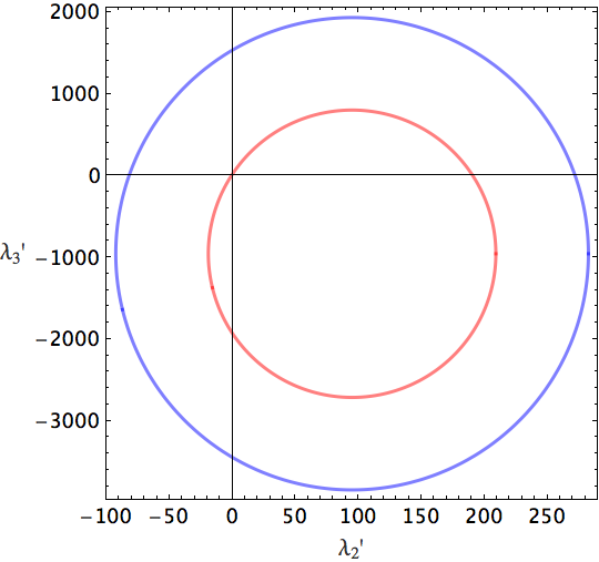
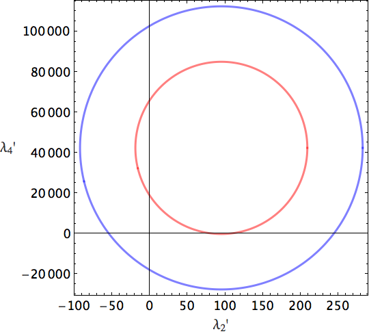
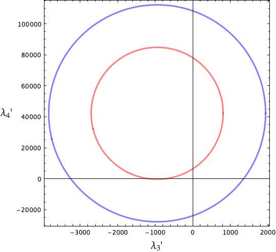
Finally, allowing both and to vary results in a lower bound for and relatively weak constraints for , plotted in Fig. 2.
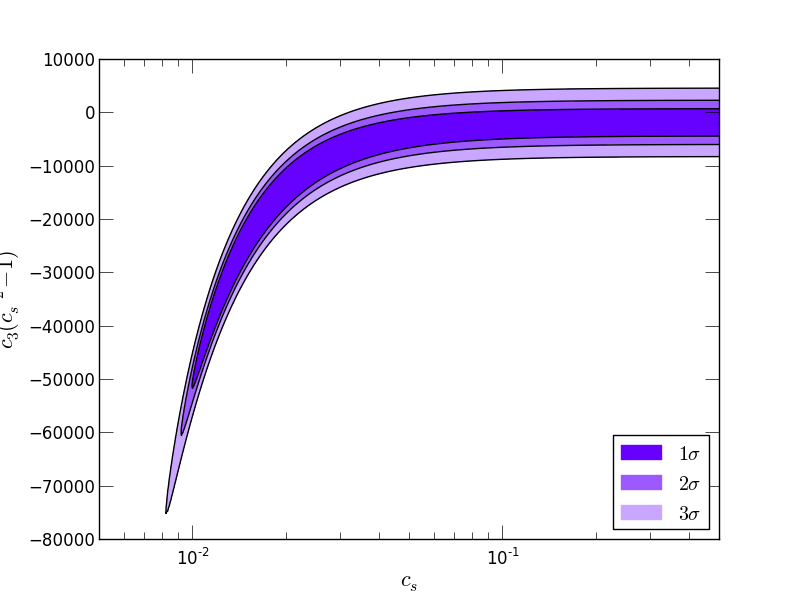
Similar bounds were reported by Senatore et al. [12]. Our construction ensures that the bounds reported above correspond to the most accurate constraints which can be achieved using this data set, because the shapes are explored using four rather than two orthogonal directions in the likelihood (29). For example, using only the leading principal component to construct the likelihood yields the constraint in the DBI model. This bound unduly weights the component of the DBI shape along this principal direction, giving an overly optimistic constraint when compared with the four-component result (35c).
Ghost inflation.—Our second example is the ‘Ghost inflation’ model proposed by Arkani-Hamed et al. [18], in which inflation is driven by a so-called ‘ghost condensate’ which spontaneously breaks Lorentz invariance in the background. The ghost condensate is described by a scalar field whose time derivative gains a nonvanishing vacuum expectation value, . This expectation value is time-independent and is not diluted as inflation proceeds.
In the effective theory, fluctuations around the background correspond to nonzero and , and the limit . This limit sets the quadratic spatial-derivative terms in (4) to zero, so that the speed of sound is formally zero. The fluctuations are nevertheless propagating modes because higher-order spatial derivative terms are present in the Lagrangian. The relevant EFT operators are
| (37a) | ||||
| (37b) | ||||
The arrangement of derivatives is identical up to a relative factor of 2 in the first term. In terms of the mass scales and we have
| (38a) | ||||
| (38b) | ||||
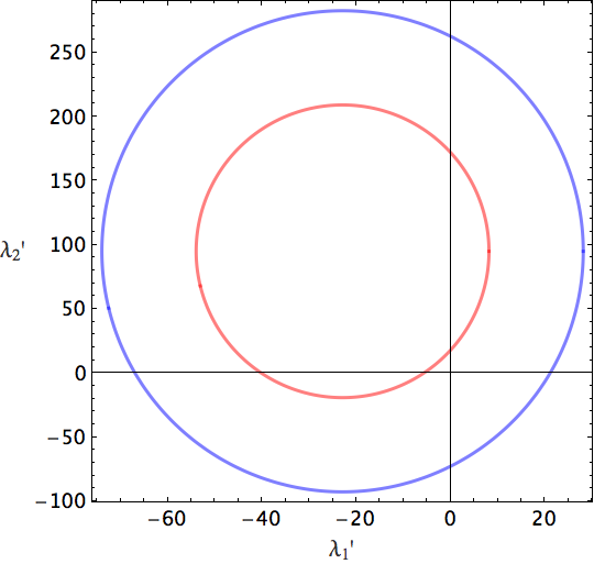
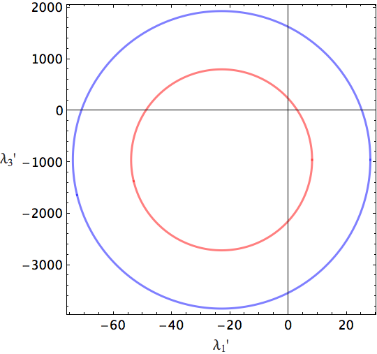
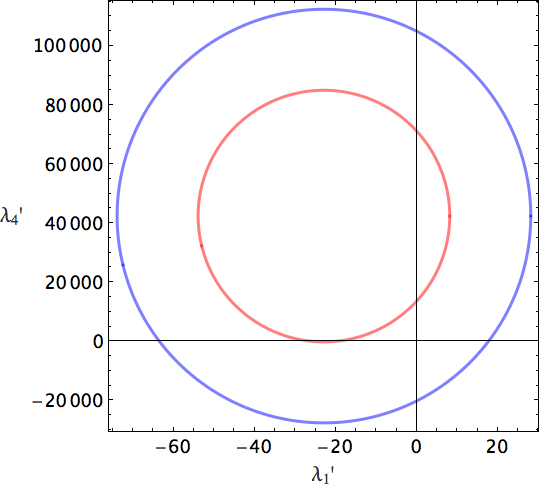
The inclusion of factors of and is purely formal, since this model technically involves the limits and . Proceeding as for the DBI model we obtain the maximum-likelihood estimates
| (39a) | ||||
| (39b) | ||||
Bartolo et al. observed that the operators (38a)–(38b) are nearly the same and chose to aggregate them into a single term operator by introducing a common mass scale , satisfying by . The corresponding to this aggregate operator [still defined to satisfy the normalization condition (9)] represents an estimate of the amplitude of the ghost-inflation bispectrum, and we label it . As explained in §3, the ghost inflation model involves fourth-order kinetic terms whose details we do not capture, and therefore the precise normalization of this estimate is uncertain. We find
| (40) |
For comparison, the Planck collaboration reported the constraint . Both estimates agree that the bispectrum in this channel is consistent with zero within . In addition, this comparison shows that, even in a case where the normalization uncertainty is important, our result matches an exact calculation within a factor of order unity.
6 Model comparison using the bispectrum
The analyses of §§4–5 determine best-fit values for the , essentially in a frequentist sense, assuming a fixed model for the underlying microphysical fluctuations. Therefore our conclusions up to this point are restricted to parameter estimation.
Within this framework it is not possible to address questions such as whether the best-fit combination for DBI inflation, Eqs. (33a)–(33b), represents a better description of the data than the best-fit combination for Ghost inflation, Eqs. (39a)–(39b). These broader questions constitute the province of model comparison. Recent work has addressed the issue of inflationary model comparison based on measurements of the two-point function of the temperature anisotropy [50]. It is much more challenging to perform a similar analysis based on the three-point function. In this section we take some steps towards this objective within the framework described in §§2–4.
For computational reasons we must impose limitations on the meaning of the term ‘model’. Conceptually this should include whatever information is necessary to specify the value of each observable. For example, the transfer matrix depends on the post-inflationary cosmological history and in a global analysis the parameters which specify this history should be varied in addition to the inflationary parameters , . However, this generates a large parameter space which is expensive to search because calculation of is time-consuming. In this analysis we will fix the transfer matrix using standard best-fit values for the post-inflationary history and address the more restricted question of which inflationary model yields a better fit for the three-point function given these assumptions.
Evidence for a model.—There is no single metric which unambiguously quantifies the evidence for or against a particular model. One choice is the ‘Bayes factor’. For a particular set of observations and a pair of models and , this is defined to be the ratio of likelihoods,
| (41) |
We use , to schematically denote two different choices of the parameters which characterize a particular model. Because and are different they may require a different number of parameters.
The probabilities represent the prior probability, for each model, that a particular parameter choice occurs. They must be chosen by hand. Where meaningful prior information exists (for example, previous measurements of a parameter) this can be encoded using these probabilities. But their arbitrariness implies that—unless it happens that is nearly independent of the —the Bayes factor is not easy to interpret. Usually, is independent of the priors only when the data are very constraining. In what follows we will see that the 9-year WMAP bispectrum data are insufficiently constraining for this to occur, so that ambiguities in the interpretation of remain.
Empirical scales are used to give meaning to the Bayes factor. Commonly used examples are due to Jeffreys or Kass & Raftery [51]. In Kass & Raftery’s prescription, in the range is considered evidence in favour of , whereas in the range is considered strong evidence and larger values of are considered decisive. Ratios for which are uninformative.
Choice of priors.—In our case the represent Lagrangian coefficients. Some prior estimates exist, but the datasets from which these were obtained are not independent of the 9-year WMAP data used in this analysis. For this reason we disregard these prior constraints, and therefore some other way must be found to justify the functional form of each prior.
If we insist that perturbation theory is valid then the should not be too large. This requirement is convenient but not obviously necessary. However, for the purpose of performing a concrete calculation we shall adopt it in what follows. In that case, the requirement that the bispectrum generated by the operator does not overwhelm the power spectrum is roughly , and therefore . This limit is helpful but gives no guidance regarding the functional form of . To explore the range of outcomes we consider two possibilities:
- •
The ‘Jeffries prior’ . This choice assigns equal probability for each decade of : that is, for to be between and , and , and so on. The Jeffries prior makes it relatively likely for to be near zero, and therefore can be regarded as conservative.1010 10 Strictly, the Jeffries prior has a divergence at . We regularize this by cutting out the region and taking to be zero within it. We have checked that our results are robust to modest changes of the boundary value. The choice of cutoff at unity is, of course, somewhat arbitrary. However, motivated by the fact that in the single parameter case corresponds to the conventionally defined parameter, we note that error bars on for single field inflationary models are at best expected to achieve values of order unity. Therefore, we shall regard as a ‘natural’ cutoff, but shall also consider the dependency of the results on the cutoff, by presenting results with cutoff at , i.e. at a value of order of the slow roll parameters.
- •
The flat prior, for which is constant. This choice assigns equal probability to each value of , and therefore makes it relatively more likely for to be large. It is less conservative than the Jeffries prior in the sense that that it enhances the probability for the Lagrangian (4) to predict observably large nongaussianities.
Examples
- •
First, consider the comparison between a trivial Gaussian model () for which and a DBI-like model () with free parameter .
Adopting the Jeffries prior, the Bayes factor between these models is
(42) The normalization factor formally satisfies , although it is regularized as described in footnote 10. We find which gives no preference for either model. Note that there is an ‘Ockham’s razor’ penalty implicit in (42), because the parameter is allowed to float over a relatively large interval. For a flat prior this Ockham penalty strongly disfavours the DBI model, producing . We conclude that the data are not sufficient to overcome the ambiguity in specifying a prior.
The Bayes factor is only one of a number of metrics which can be used to assess goodness of fit. Another is the Akaike ‘information criterion’, defined by , where measures the number of parameters in the model and is a proxy for the ‘Ockham razor’ penalty of Eq. (41). The model with smallest is preferred. We find , which implies a preference for the trivial Gaussian model in comparison to a model with nonzero . The same preference is found if we allow any other single Lagrangian parameter to be nonzero.
- •
Next, consider a third DBI-like model in which the two parameters and (or, equivalently, the parameters and in the notation of §5) are allowed to float. We find
Jeffries prior difference , cutoff=1 , cutoff=0.01 vs. vs. The Akaike information criterion prefers to , but to . Therefore the trivial Gaussian model is preferred overall, but if we discard this option then the information criterion prefers a two-parameter fit () to a single-parameter fit ().
The Bayes factors are inconclusive, but it could be argued that they show a weak preference for the opposite conclusion. We compute the Bayes factor using two different choices for the regularization of the Jeffries prior; see footnote 10 on p. 10. A smaller cutoff increases the weight of probability for the to be near zero, and therefore decreases the probability that the model generates an observable signature. As we increase the lower limit for the parameters to the ‘natural’ level , the Bayes factor does not strongly discriminate between a two- or three-parameter fit. However, it does marginally begin to disfavour a two-parameter fit () compared to the trivial model (). Therefore it appears that a fit for a DBI-like model using more than two parameters becomes mildly in tension with the data for ‘natural’ choices of the dimensionless scales .
The apparent discrepancy with the Akaike information criterion should be ascribed to a stronger ‘Ockham’ or complexity penalty in the Bayes factor. The information criterion down-weights each model by a fixed amount depending on the number of parameters, whereas the Bayes factor attempts to account for the increased volume of parameter space which becomes available. For example, using a flat prior instead of the Jeffries prior very strongly disfavours the models and .
7 Discussion and conclusions
The availability of high-quality maps of the CMB temperature anisotropy from the WMAP and Planck missions means that it has become feasible to search for primordial three-point correlations. Such correlations are typically predicted by any scenario in which the fluctuations have an inflationary origin, due to microphysical three-body interactions among the light, active degrees of freedom of the inflationary epoch. If detected, their precise form could provide decisive evidence in favour of the inflationary hypothesis.
Unfortunately, due to issues of computational complexity, it is not yet possible to perform a blind search for these primordial three-point correlations. Instead, we must search for signals which we have some prior reason to believe may be present in the data. Therefore the amount of information we manage to extract depends on which signals we choose to look for.
In this paper we have made a systematic search of the 9-year WMAP data for correlations which could be produced in a very general model of single-field inflation, under the assumption that the background evolution is smooth, yielding corresponding smooth and nearly scale-invariant correlation functions. This excludes models which contain sharp features or oscillations [52, 53, 54, 55, 56, 57, 58, 59, 60, 61]. It also excludes models in which significant three-point correlations are generated by differences of evolution between regions of the universe separated by super-Hubble distances. Correlations generated by this mechanism are generally most significant in the ‘squeezed’ or soft limit, where the correlation is between fluctuations on very disparate scales. Such correlations have been disfavoured by analysis of the Planck2013 data release [1]. By comparison, the 9-year WMAP data achieve a smaller signal-to-noise for such configurations. The difference between the 9-year WMAP and Planck2013 datasets is less pronounced for the momentum configurations which we probe, with for example error bars on improving from to .
The essential steps of our analysis were assembled in §§2–4. We begin with an effective field theory which parametrizes the unknown details of three-body interactions between inflaton fluctuations, but preserves nonlinearly realized Lorentz invariance. The effective theory is agnostic regarding the physical mechanism which underlies inflation. We compute the bispectrum generated by each operator in the effective theory, and break these into principal components using a Fisher-matrix approach. The amplitude of each principal component is recovered from the data, after which the results can be translated into constraints on the mass scales which appeared in the original effective theory. We find that no significant deviation from Gaussianity has been detected in any region of the inflationary parameter space. This conclusion is consistent with previous analyses of the 9-year WMAP and Planck2013 datasets.
Our principal components are similar to those obtained by Byun & Bean, who forecast the constraints which could be obtained from a Planck-like survey [39]. We find that the best-constrained principal direction exhibits similarities to (in order) the flattened, orthogonal and ‘Galileon’ templates. A fourth principal direction is more complex, but at best weakly constrained.
The large space of models which fit into the class of single-field scenarios invites attempts to identify best-fitting regions. To approach this problem we use the framework of Bayesian model comparison. The results are at best weakly significant, but tend to disfavour models with more parameters when compared to simpler cases with zero or one parameter. This is not surprising given that the amplitude of each principal direction is consistent with zero. However, it should be borne in mind that our analysis is restricted to smooth and nearly scale-invariant bispectra. It is possible that a significant signal of a different type is hidden in the data. In some cases, -point functions of this type can be described within the framework of effective field theory [15]. The analysis developed in §§2–4 could be applied immediately to such scenarios given a suitable choice of basis functions .
Acknowledgements
It is a pleasure to thank Andrew Liddle for many helpful discussions and useful comments on an advance draft of this manuscript. We are also grateful to Raquel Ribeiro and Sébastien Renaux-Petel for discussions which helped motivate the approach we developed in this work.
Some numerical presented in this paper were obtained using the COSMOS supercomputer, which is funded by STFC, HEFCE and SGI. Other numerical computations were carried out on the Sciama High Performance Compute (HPC) cluster which is supported by the ICG, SEPNet and the University of Portsmouth. DR and DS acknowledge support from the Science and Technology Facilities Council [grant number ST/I000976/1]. GA is supported by STFC grant ST/I506029/1. DS also acknowledges support from the Leverhulme Trust. The research leading to these results has received funding from the European Research Council under the European Union’s Seventh Framework Programme (FP/2007–2013) / ERC Grant Agreement No. [308082].
Appendix A Three-point functions for the EFT operators
In this Appendix we briefly recapitulate the calculation of the three-point functions corresponding to each operator in the effective Lagrangian (4). The principal tool is Schwinger’s formulation of ‘in–in’ expectation values and the corresponding expansion into diagrams due to Keldysh [62, 63, 64, 65]. The technique was applied to general relativity by Jordan, who used it to study the effective equations of motion obtained by integrating out quantum fluctuations [66]. It was imported into cosmology by Calzetta & Hu [67] and applied to inflation by Maldacena and subsequent authors [26, 30, 68].
In–in calculations.—The objective is to calculate the expectation value of a given operator at some time , given that the system develops from a specified state (the ‘in’-state) at very early times. This expectation value is
| (43) |
where the subscript ‘’ is used to denote evaluation of at time . In the present case, will correspond to a product of field operators evaluated at the same time but at distinct spatial positions.
Inserting a complete set of intermediate states labelled by the three-dimensional field configuration at some arbitrary time , we conclude
| (44) |
where the measure denotes integration over all field configurations. Each overlap in (44) can be written as a conventional Feynman path integral, with the integration running over all field histories which are consistent with the in-state in the far past, and which coincide with the configuration at time . The result is
| (45) |
with the independent integrations , running over field histories which are compatible with the in-state but are unrestricted at late times. Eq. (45) admits an expansion into diagrams in which the Green’s functions connecting only ‘’ or only ‘’ fields obey the usual Feynman boundary conditions, but are augmented by Green’s functions which mix the ‘’ and ‘’ labels and whose boundary conditions are determined by the -function. For further details, see Ref. [30].
Mode functions.—It was explained in §3 that we approximate the mode functions as Hankel functions of order 3/2. Analytically, this corresponds to building Green’s functions from the mode function
| (46) |
and its complex conjugate. In this formula, is the conformal time and is a ‘generalized’ speed of sound. In a model without fourth-derivative kinetic terms this will usually be the phase velocity, determined from the ratio of coefficients of the spatial and temporal kinetic terms. In other cases it may bear less relation to what would normally be thought of as a phase velocity. Our notation coincides with that of Refs. [13, 14], to which we refer for further details; see especially the discussion below Eq. (2.6) in Ref. [14]. In writing Eq. (46) we have assumed that the in-state contains zero particles, corresponding the ‘Bunch–Davies’ vacuum.
With these choices, the three-point functions corresponding to the EFT operators in (4) are:
- •
- •
- •
- •
- •
- •
- •
- •
- •
- •
- •
where
with , , and .
References
- (1) Planck Collaboration Collaboration, P. Ade et al., Planck 2013 Results. XXIV. Constraints on primordial non-Gaussianity, arXiv:1303.5084.
- (2) WMAP Collaboration Collaboration, G. Hinshaw et al., Nine-Year Wilkinson Microwave Anisotropy Probe (WMAP) Observations: Cosmological Parameter Results, arXiv:1212.5226.
- (3) C. Cheung, P. Creminelli, A. L. Fitzpatrick, J. Kaplan, and L. Senatore, The Effective Field Theory of Inflation, JHEP 0803 (2008) 014, [arXiv:0709.0293].
- (4) S. Weinberg, Adiabatic modes in cosmology, Phys.Rev. D67 (2003) 123504, [astro-ph/0302326].
- (5) S. Weinberg, Can non-adiabatic perturbations arise after single-field inflation?, Phys.Rev. D70 (2004) 043541, [astro-ph/0401313].
- (6) S. Weinberg, Must cosmological perturbations remain non-adiabatic after multi-field inflation?, Phys.Rev. D70 (2004) 083522, [astro-ph/0405397].
- (7) J. Meyers and N. Sivanandam, Non-Gaussianities in Multifield Inflation: Superhorizon Evolution, Adiabaticity, and the Fate of fnl, Phys.Rev. D83 (2011) 103517, [arXiv:1011.4934].
- (8) J. Elliston, D. J. Mulryne, D. Seery, and R. Tavakol, Evolution of fNL to the adiabatic limit, JCAP 1111 (2011) 005, [arXiv:1106.2153].
- (9) P. Creminelli, M. A. Luty, A. Nicolis, and L. Senatore, Starting the Universe: Stable Violation of the Null Energy Condition and Non-standard Cosmologies, JHEP 0612 (2006) 080, [hep-th/0606090].
- (10) C. Cheung, A. L. Fitzpatrick, J. Kaplan, and L. Senatore, On the consistency relation of the 3-point function in single field inflation, JCAP 0802 (2008) 021, [arXiv:0709.0295].
- (11) S. Weinberg, Effective Field Theory for Inflation, Phys.Rev. D77 (2008) 123541, [arXiv:0804.4291].
- (12) L. Senatore, K. M. Smith, and M. Zaldarriaga, Non-Gaussianities in Single Field Inflation and their Optimal Limits from the WMAP 5-year Data, JCAP 1001 (2010) 028, [arXiv:0905.3746].
- (13) N. Bartolo, M. Fasiello, S. Matarrese, and A. Riotto, Large non-Gaussianities in the Effective Field Theory Approach to Single-Field Inflation: the Bispectrum, JCAP 1008 (2010) 008, [arXiv:1004.0893].
- (14) N. Bartolo, M. Fasiello, S. Matarrese, and A. Riotto, Large non-Gaussianities in the Effective Field Theory Approach to Single-Field Inflation: the Trispectrum, JCAP 1009 (2010) 035, [arXiv:1006.5411].
- (15) N. Bartolo, D. Cannone, and S. Matarrese, The Effective Field Theory of Inflation Models with Sharp Features, JCAP 1310 (2013) 038, [arXiv:1307.3483].
- (16) P. Adshead, W. Hu, and V. Miranda, Bispectrum in Single-Field Inflation Beyond Slow-Roll, Phys.Rev. D88 (2013) 023507, [arXiv:1303.7004].
- (17) M. Alishahiha, E. Silverstein, and D. Tong, DBI in the sky, Phys.Rev. D70 (2004) 123505, [hep-th/0404084].
- (18) N. Arkani-Hamed, P. Creminelli, S. Mukohyama, and M. Zaldarriaga, Ghost inflation, JCAP 0404 (2004) 001, [hep-th/0312100].
- (19) M. Dias, R. H. Ribeiro, and D. Seery, The δN formula is the dynamical renormalization group, JCAP 1310 (2013) 062, [arXiv:1210.7800].
- (20) V. Assassi, D. Baumann, and D. Green, Symmetries and Loops in Inflation, JHEP 1302 (2013) 151, [arXiv:1210.7792].
- (21) L. Senatore and M. Zaldarriaga, On Loops in Inflation, JHEP 1012 (2010) 008, [arXiv:0912.2734].
- (22) L. Senatore and M. Zaldarriaga, A Naturally Large Four-Point Function in Single Field Inflation, JCAP 1101 (2011) 003, [arXiv:1004.1201].
- (23) L. Senatore and M. Zaldarriaga, The Effective Field Theory of Multifield Inflation, JHEP 1204 (2012) 024, [arXiv:1009.2093].
- (24) D. Baumann and D. Green, Equilateral Non-Gaussianity and New Physics on the Horizon, JCAP 1109 (2011) 014, [arXiv:1102.5343].
- (25) D. Baumann, L. Senatore, and M. Zaldarriaga, Scale-Invariance and the Strong Coupling Problem, JCAP 1105 (2011) 004, [arXiv:1101.3320].
- (26) J. M. Maldacena, Non-Gaussian features of primordial fluctuations in single field inflationary models, JHEP 05 (2003) 013, [astro-ph/0210603].
- (27) P. Creminelli, On non-Gaussianities in single-field inflation, JCAP 0310 (2003) 003, [astro-ph/0306122].
- (28) D. Seery and J. E. Lidsey, Primordial non-gaussianities in single field inflation, JCAP 0506 (2005) 003, [astro-ph/0503692].
- (29) D. Seery and J. E. Lidsey, Primordial non-gaussianities from multiple-field inflation, JCAP 0509 (2005) 011, [astro-ph/0506056].
- (30) S. Weinberg, Quantum contributions to cosmological correlations, Phys.Rev. D72 (2005) 043514, [hep-th/0506236].
- (31) X. Chen, M.-x. Huang, S. Kachru, and G. Shiu, Observational signatures and non-Gaussianities of general single field inflation, JCAP 0701 (2007) 002, [hep-th/0605045].
- (32) C. Burrage, R. H. Ribeiro, and D. Seery, Large slow-roll corrections to the bispectrum of noncanonical inflation, JCAP 1107 (2011) 032, [arXiv:1103.4126].
- (33) J. Elliston, D. Seery, and R. Tavakol, The inflationary bispectrum with curved field-space, JCAP 1211 (2012) 060, [arXiv:1208.6011].
- (34) J. Fergusson, M. Liguori, and E. Shellard, General CMB and Primordial Bispectrum Estimation I: Mode Expansion, Map-Making and Measures of , Phys.Rev. D82 (2010) 023502, [arXiv:0912.5516].
- (35) J. Fergusson, M. Liguori, and E. Shellard, The CMB Bispectrum, JCAP 1212 (2012) 032, [arXiv:1006.1642].
- (36) J. Fergusson, D. Regan, and E. Shellard, Rapid Separable Analysis of Higher Order Correlators in Large Scale Structure, Phys.Rev. D86 (2012) 063511, [arXiv:1008.1730].
- (37) J. Fergusson, D. Regan, and E. Shellard, Optimal Trispectrum Estimators and WMAP Constraints, arXiv:1012.6039.
- (38) D. Regan, E. Shellard, and J. Fergusson, General CMB and Primordial Trispectrum Estimation, Phys.Rev. D82 (2010) 023520, [arXiv:1004.2915].
- (39) J. Byun and R. Bean, Non-Gaussian Shape Recognition, JCAP 1309 (2013) 026, [arXiv:1303.3050].
- (40) T. Battefeld and J. Grieb, Anatomy of bispectra in general single-field inflation – modal expansions, JCAP 1112 (2011) 003, [arXiv:1110.1369].
- (41) D. Regan, P. Mukherjee, and D. Seery, General CMB bispectrum analysis using wavelets and separable modes, arXiv:1302.5631.
- (42) D. Regan, M. Gosenca, and D. Seery, Constraining the WMAP9 bispectrum and trispectrum with needlets, arXiv:1310.8617.
- (43) J. Fergusson and E. Shellard, The shape of primordial non-Gaussianity and the CMB bispectrum, Phys.Rev. D80 (2009) 043510, [arXiv:0812.3413].
- (44) M. Vallisneri, Use and abuse of the Fisher information matrix in the assessment of gravitational-wave parameter-estimation prospects, Phys.Rev. D77 (2008) 042001, [gr-qc/0703086].
- (45) D. Babich, P. Creminelli, and M. Zaldarriaga, The Shape of non-Gaussianities, JCAP 0408 (2004) 009, [astro-ph/0405356].
- (46) P. D. Meerburg, J. P. van der Schaar, and P. S. Corasaniti, Signatures of Initial State Modifications on Bispectrum Statistics, JCAP 0905 (2009) 018, [arXiv:0901.4044].
- (47) P. Creminelli, G. D’Amico, M. Musso, J. Norena, and E. Trincherini, Galilean symmetry in the effective theory of inflation: new shapes of non-Gaussianity, JCAP 1102 (2011) 006, [arXiv:1011.3004].
- (48) R. H. Ribeiro and D. Seery, Decoding the bispectrum of single-field inflation, JCAP 1110 (2011) 027, [arXiv:1108.3839].
- (49) WMAP Collaboration, C. Bennett et al., Nine-Year Wilkinson Microwave Anisotropy Probe (WMAP) Observations: Final Maps and Results, Astrophys.J.Suppl. 208 (2013) 20, [arXiv:1212.5225].
- (50) J. Martin, C. Ringeval, R. Trotta, and V. Vennin, The Best Inflationary Models After Planck, arXiv:1312.3529.
- (51) R. E. Kass and A. E. Raftery, Bayes factors, Journal of the American Statistical Association 90 (1995), no. 430 773–795, [http://amstat.tandfonline.com/doi/pdf/10.1080/01621459.1995.10476572].
- (52) A. A. Starobinsky, Spectrum of adiabatic perturbations in the universe when there are singularities in the inflation potential, JETP Lett. 55 (1992) 489–494.
- (53) J. A. Adams, G. G. Ross, and S. Sarkar, Multiple inflation, Nucl.Phys. B503 (1997) 405–425, [hep-ph/9704286].
- (54) J. A. Adams, B. Cresswell, and R. Easther, Inflationary perturbations from a potential with a step, Phys.Rev. D64 (2001) 123514, [astro-ph/0102236].
- (55) G. Hailu and S.-H. H. Tye, Structures in the Gauge/Gravity Duality Cascade, JHEP 0708 (2007) 009, [hep-th/0611353].
- (56) R. Bean, X. Chen, G. Hailu, S.-H. H. Tye, and J. Xu, Duality Cascade in Brane Inflation, JCAP 0803 (2008) 026, [arXiv:0802.0491].
- (57) A. Achucarro, J.-O. Gong, S. Hardeman, G. A. Palma, and S. P. Patil, Features of heavy physics in the CMB power spectrum, JCAP 1101 (2011) 030, [arXiv:1010.3693].
- (58) M. Joy, V. Sahni, and A. A. Starobinsky, A New Universal Local Feature in the Inflationary Perturbation Spectrum, Phys.Rev. D77 (2008) 023514, [arXiv:0711.1585].
- (59) S. Hotchkiss and S. Sarkar, Non-Gaussianity from violation of slow-roll in multiple inflation, JCAP 1005 (2010) 024, [arXiv:0910.3373].
- (60) M. Nakashima, R. Saito, Y.-i. Takamizu, and J. Yokoyama, The effect of varying sound velocity on primordial curvature perturbations, Prog.Theor.Phys. 125 (2011) 1035–1052, [arXiv:1009.4394].
- (61) P. Adshead, W. Hu, C. Dvorkin, and H. V. Peiris, Fast Computation of Bispectrum Features with Generalized Slow Roll, Phys.Rev. D84 (2011) 043519, [arXiv:1102.3435].
- (62) J. S. Schwinger, Brownian motion of a quantum oscillator, J.Math.Phys. 2 (1961) 407–432.
- (63) P. M. Bakshi and K. T. Mahanthappa, Expectation value formalism in quantum field theory. 1., J.Math.Phys. 4 (1963) 1–11.
- (64) P. M. Bakshi and K. T. Mahanthappa, Expectation value formalism in quantum field theory. 2., J.Math.Phys. 4 (1963) 12–16.
- (65) L. Keldysh, Diagram technique for nonequilibrium processes, Zh.Eksp.Teor.Fiz. 47 (1964) 1515–1527.
- (66) R. Jordan, Effective Field Equations for Expectation Values, Phys.Rev. D33 (1986) 444–454.
- (67) E. Calzetta and B. Hu, Closed Time Path Functional Formalism in Curved Space-Time: Application to Cosmological Back Reaction Problems, Phys.Rev. D35 (1987) 495.
- (68) S. Weinberg, Quantum contributions to cosmological correlations. II. Can these corrections become large?, Phys.Rev. D74 (2006) 023508, [hep-th/0605244].