跳到论文正文
W Papers独立论文阅读器 arXiv:1403.3320 论文正文 计算阅读时间 · 0%
引用这篇论文根据当前论文元数据生成,正式投稿前建议核对。


License: arXiv.org perpetual non-exclusive license
arXiv:1403.3320v7 [math.NA] 01 Mar 2016

Numerical Approaches for Linear Left-invariant Diffusions on S​E​(2)SE(2), their Comparison to Exact Solutions, and their Applications in Retinal Imaging.

Jiong Zhang Affiliation: 1, Note: Corresponding and joint main authors. Email address: J.Zhang1@tue.nl (J. Zhang), R.Duits@tue.nl (R. Duits)    Remco Duits∗ Affiliation: 1, Affiliation: 2,    Gonzalo Sanguinetti and Bart M. ter Haar Romeny Affiliation: 3, Address: 1Department of Biomedical Engineering, Biomedical Image Analysis (BMIA)
2Department of Mathematics and Computer Science, Image Science and Technology (IST/e)
1,2Eindhoven University of Technology, P.O. Box 513, 5600 MB, Eindhoven, The Netherlands.
3Northeastern University, Shenyang, China.
Abstract

Left-invariant PDE-evolutions on the roto-translation group S​E​(2)SE(2) (and their resolvent equations) have been widely studied in the fields of cortical modeling and image analysis. They include hypo-elliptic diffusion (for contour enhancement) proposed by Citti &\& Sarti, and Petitot, and they include the direction process (for contour completion) proposed by Mumford. This paper presents a thorough study and comparison of the many numerical approaches, which, remarkably, are missing in the literature. Existing numerical approaches can be classified into 3 categories: Finite difference methods, Fourier based methods (equivalent to S​E​(2)SE(2)-Fourier methods), and stochastic methods (Monte Carlo simulations). There are also 3 types of exact solutions to the PDE-evolutions that were derived explicitly (in the spatial Fourier domain) in previous works by Duits and van Almsick in 2005. Here we provide an overview of these 3 types of exact solutions and explain how they relate to each of the 3 numerical approaches. We compute relative errors of all numerical approaches to the exact solutions, and the Fourier based methods show us the best performance with smallest relative errors. We also provide an improvement of Mathematica algorithms for evaluating Mathieu-functions, crucial in implementations of the exact solutions. Furthermore, we include an asymptotical analysis of the singularities within the kernels and we propose a probabilistic extension of underlying stochastic processes that overcomes the singular behavior in the origin of time-integrated kernels. Finally, we show retinal imaging applications of combining left-invariant PDE-evolutions with invertible orientation scores.

keywords
Brownian motion, Euclidean motion group, PDE’s on S​E​(2)SE(2), Mathieu operators, contour completion, contour enhancement, retinal imaging

1 Introduction

Hubel and Wiesel [38] discovered that certain visual cells in cats’ striate cortex have a directional preference. It has turned out that there exists an intriguing and extremely precise spatial and directional organization into so-called cortical hypercolumns, see Figure 1. A hypercolumn can be interpreted as a “visual pixel”, representing the optical world at a single location, neatly decomposed into a complete set of orientations. Moreover, correlated horizontal connections run parallel to the cortical surface and link columns across the spatial visual field with a shared orientation preference, allowing cells to combine visual information from spatially separated receptive fields. Synaptic physiological studies of these horizontal pathways in cats’ striate cortex show that neurons with aligned receptive field sites excite each other [15]. Apparently, the visual system not only constructs a score of local orientations, but also accounts for context and alignment by excitation and inhibition a priori, which can be modeled by left-invariant PDE’s and ODE’s on S​E​(2)SE(2) [47, 19, 21, 24, 12, 6, 11, 17, 43, 50, 51, 58, 25, 26, 29, 32, 8, 46].

Refer to caption
Figure 1: The orientation columns in the primary visual cortex.

Motivated by the orientation-selective cells, so-called orientation scores are constructed by lifting all elongated structures (in 2D images) along an extra orientation dimension [41, 21, 24]. The main advantage of using the orientation score is that we can disentangle the elongated structures involved in a crossing allowing for a crossing preserving flow.

Invertibility of the transform between image and score is of vital importance, to both tracking [10] and enhancement[52, 33], as we do not want to tamper data-evidence in our continuous coherent state transform[3, 58] before actual processing takes place. This is a key advantage over related state-of-the-art methods[7, 43, 58, 12, 19].
Refer to caption
Figure 2: Real part of an orientation score of an example image.

Invertible orientation scores (see Figure 2) are obtained via a unitary transform between the space of disk-limited images L2%(R2):={f∈L2(R2)|support{ℱℛ∈{}⊂ℬ0,%}\mdmathbb{L}_{2}^{\varrho}(\mdmathbb{R}^{2}):=\{f\in\mdmathbb{L}_{2}(\mdmathbb{R}^{2})\;|\;\textrm{support}\{\mathcall{F}_{\mdmathbb{R}^{2}}f\}\subset B_{\textbf{0},\varrho}\} (with %>0\varrho>0 close to the Nyquist frequency and B0,%={!∈R2|‖!‖≤%}B_{\textbf{0},\varrho}=\{\mbox{\boldmath$\omega$}\in\mdmathbb{R}^{2}\;|\;\|\mbox{\boldmath$\omega$}\|\leq\varrho\}), and the space of orientation scores. The space of orientation scores is a specific reproducing kernel vector subspace [21, 4, 3] of L2​(R2×S1)\mdmathbb{L}_{2}(\mdmathbb{R}^{2}\times S^{1}), see Appendix A for the connection with continuous wavelet theory. The transform from an image ff to an orientation score Uf:=𝒲{U_{f}:=\mathcall{W}f is constructed via an anisotropic convolution kernel ∈L2​(R2)∩L1​(R2)\psi\in\mdmathbb{L}_{2}(\mdmathbb{R}^{2})\!\cap\!\mdmathbb{L}_{1}(\mdmathbb{R}^{2}):

Uf(x,�)=(𝒲[{])(x,�)=∫ℛ∈ ​(R�−∞​(y−x))¯{(y)⌈y,U_{f}(\textbf{x},\theta)=(\mathcall{W}[f])(\textbf{x},\theta)=\int_{\mdmathbb{R}^{2}}\overline{\psi(\textbf{R}_{\theta}^{-1}(\textbf{y}{-\textbf{x}}))}f(\textbf{y})d\textbf{y}, (1)

where 𝒲\mathcall{W} denotes the transform and R�=(cos⁡�−sin⁡�sin⁡�cos⁡�).\small\textbf{R}_{\theta}=\left(\begin{array}[]{ccc}\cos\theta&-\sin\theta\\ \sin\theta&\cos\theta\\ \end{array}\right). Exact reconstruction is obtained by

f(x)=(𝒲∗[𝒰{])(x)=(ℱℛ∈−∞[ℳ−∞ℱℛ∈[∞∈�∫′∈�(�∗𝒰{(⋅,�))⌈�]])(x),\displaystyle f(\textbf{x})=(\mathcall{W}^{*}[U_{f}])(\textbf{x})=\left(\mathcall{F}_{\mdmathbb{R}^{2}}^{-1}\left[M^{-1}\mathcall{F}_{\mdmathbb{R}^{2}}\left[\frac{1}{2\pi}\int_{0}^{2\pi}({}_{\theta}*U_{f}(\cdot,\theta))d\theta\right]\right]\right)(\textbf{x}), (2)

for all x∈R2\textbf{x}\in\mdmathbb{R}^{2}, where ℱℛ∈\mathcall{F}_{\mdmathbb{R}^{2}} is the unitary Fourier transform on L2​(R2)\mdmathbb{L}_{2}(\mdmathbb{R}^{2}) and M∈C⁡(R2,R)M\in C(\mdmathbb{R}^{2},\mdmathbb{R}) is given by M⁡(!)=∫02​�| ^​(R�−1​!)|2​𝑑�M(\boldsymbol{\omega})=\int_{0}^{2\pi}|\hat{\psi}(\textbf{R}_{\theta}^{-1}\boldsymbol{\omega})|^{2}d\theta for all !∈R2\boldsymbol{\omega}\in\mdmathbb{R}^{2}, with ^:=ℱℛ∈​ \hat{\psi}:=\mathcall{F}_{\mdmathbb{R}^{2}}\psi, (x)�= (R�−1x){}_{\theta}(\textbf{x})=\psi(R_{\theta}^{-1}\textbf{x}). Furthermore, 𝒲∗\mathcall{W}^{*} denotes the adjoint of wavelet transform 𝒲:ℒ∈​(ℛ∈)→𝒞𝒦𝒮ℰ⁡(∈)\mathcall{W}:\mdmathbb{L}_{2}(\mdmathbb{R}^{2})\rightarrow\mdmathbb{C}_{K}^{SE(2)}, where the reproducing kernel norm on the space of orientation scores, CKS​E​(2)={𝒲{|{∈ℒ∈(ℛ∈)}\mdmathbb{C}_{K}^{SE(2)}=\{\mathcall{W}f\;|\;f\in\mdmathbb{L}_{2}(\mdmathbb{R}^{2})\}, is explicitly characterized in [24, Thm.4, Eq. 11]. Well-posedness of the reconstruction is controlled by MM[24, 10]. For details see Appendix A. Regarding the choice of \psi in our algorithms, we rely on the wavelets proposed in [21, ch:4.6.1],[10].

In this article, the invertible orientation scores serve as the initial condition of left-invariant (non-) linear PDE evolutions on the rotation-translation group R2𝑜S​O​(2)≡S​E​(2)\mdmathbb{R}^{2}\rtimes SO(2)\equiv SE(2), where by definition,
Rd𝑜Sd−1:=Rd𝑜S​O​(d)/({0}×S​O​(d−1))\mdmathbb{R}^{d}\rtimes S^{d-1}:=\mdmathbb{R}^{d}\rtimes SO(d)/(\{0\}\times SO(d-1)). Now in our case d=2d=2, so R2𝑜S1=R2𝑜S​O​(2)\mdmathbb{R}^{2}\rtimes S^{1}=\mdmathbb{R}^{2}\rtimes SO(2) and we identify rotations with orientations. The primary focus of this article, however, is on the numerics and comparison to the exact solutions of linear left-invariant PDE’s on S​E​(2)SE(2). Here by left-invariance and linearity we can restrict ourselves in our numerical analysis to the impulse response, where the initial condition is equal to �e=�0x⊗�0y⊗�0�\delta_{e}=\delta_{0}^{x}\otimes\delta_{0}^{y}\otimes\delta_{0}^{\theta}, where ⊗\otimes denotes the tensor product in distributional sense.

In fact, we consider all linear, second order, left-invariant evolution equations and their resolvents on L2​(R2𝑜S1)≡L2​(S​E​(2))\mdmathbb{L}_{2}(\mdmathbb{R}^{2}\rtimes S^{1})\equiv\mdmathbb{L}_{2}(SE(2)), which actually correspond to the forward Kolmogorov equations of left-invariant stochastic processes. Specifically, there are two types of stochastic processes we will investigate in the field of imaging and vision:

  • •

    The contour enhancement process as proposed by Citti et al.[19] in the cortical modeling.

  • •

    The contour completion process as proposed by Mumford [46] also called the direction process.

In image analysis, the difference between the two processes is that the contour enhancement focuses on the de-noising of elongated structures, while the contour completion aims for bridging the gap of interrupted contours since it contains a convection part.

Although not being considered in this article, we mention related 3D (S​E​(3))(SE(3)) extensions of these processes and applications (primarily in DW-MRI) in [20, 45, 48]. Most of our numerical findings in this article apply to these S​E​(3)SE(3) extensions as well.

Many numerical approaches for implementing left-invariant PDE’s on S​E​(2)SE(2) have been investigated intensively in the fields of cortical modeling and image analysis. Petitot introduced a geometrical model for the visual cortex V1 [47], further refined to the S​E​(2)SE(2) setting by Citti and Sarti [19]. A method for completing the boundaries of partially occluded objects based on stochastic completion fields was proposed by Zweck and Williams[58]. Also, Barbieri et al.[8] proposed a left-invariant cortical contour perception and motion integration model within a 5D contact manifold. In the recent work of Boscain et al.[12], a numerical algorithm for integration of a hypoelliptic diffusion equation on the group of translations and discrete rotations S​E​(2,N)SE(2,N) is investigated. Moreover, some numerical schemes were also proposed by August et al. [6, 7] to understand the direction process for curvilinear structure in images. Duits, van Almsick and Franken[25, 26, 29, 32, 56, 21] also investigated different models based on Lie groups theory, with many applications to medical imaging.

The numerical schemes for left-invariant PDE’s on S​E​(2)SE(2) can be categorized into 3 approaches:

  • •

    Finite difference approaches.

  • •

    Fourier based approaches, including S​E​(2)SE(2)-Fourier methods.

  • •

    Stochastic approaches.

Recently, several explicit representations of exact solutions were derived [27, 28, 25, 56, 29, 2]. In this paper we will set up a structured framework to compare all the numerical approaches to the exact solutions.
Contributions of the article: In this article, we:

  • •

    compare all numerical approaches (finite difference methods, a stochastic method based on Monte Carlo simulation and Fourier based methods) to the exact solution for contour enhancement/completion. We show that the Fourier based approaches perform best and we also explain this theoretically in Theorem 5.4;

  • •

    provide a concise overview of all exact approaches;

  • •

    implement exact solutions, including improvements of Mathieu-function evaluations in Mathematica;

  • •

    establish explicit connections between exact and numerical approaches for contour enhancement;

  • •

    analyze the poles/singularities of the resolvent kernels;

  • •

    propose a new probabilistic time integration to overcome the poles, and we prove this via new simple asymptotic formulas for the corresponding kernels that we present in this article;

  • •

    show benefits of the newly proposed time integration in contour completion via stochastic completion fields [58];

  • •

    analyze errors when using the DFT (Discrete Fourier Transform) instead of the CFT (Continuous Fourier Transform) to transform exact formulas in the spatial Fourier domain to the S​E​(2)SE(2) domain;

  • •

    apply left-invariant evolutions as preprocessing before tracking the retinal vasculature via the ETOS-algorithm [10] in optical imaging of the eye.

Structure of the article: In Section 2 we will briefly describe the theory of the S​E​(2)SE(2) group and left-invariant vector fields. Subsequently, in Section 3 we will discuss the linear time dependent OPEN(convection-)\mbox{(}\text{convection-}) diffusion processes on S​E​(2)SE(2) and the corresponding resolvent equation for contour enhancement and contour completion. In Subsection 3.3 we provide improved kernels via iteration of resolvent operators and give a probabilistic interpretation. Then we show the benefit in stochastic completion fields. For completeness, the fundamental solution and underlying probability theory for contour enhancement/completion is explained in Subsection 3.4.

In Section 4 we will give the full implementations for all our numerical schemes for contour enhancement/completion, i.e. explicit and implicit finite difference schemes, numerical Fourier based techniques, and the Monte-Carlo simulation of the stochastic approaches. Then, in Section 5, we will provide a new concise overview of all three exact approaches in the general left-invariant PDE-setting. Direct relations between the exact solution representations and the numerical approaches are also given in this section. After that, we will provide experiments with different parameter settings and show the performance of all different numerical approaches compared to the exact solutions. Finally, we conclude our paper with applications on retinal images to show the power of our multi-orientation left-invariant diffusion with an application on complex vessel enhancement, i.e. in the presence of crossings and bifurcations.

2 The S​E​(2)SE(2) Group and Left-invariant Vector Fields

2.1 The Euclidean Motion Group S​E​(2)SE(2) and Representations

An orientation score U:S​E​(2)→CU:SE(2)\to\mdmathbb{C} is defined on the Euclidean motion group S​E​(2)=R2𝑜S1SE(2)=\mdmathbb{R}^{2}\rtimes S^{1}. The group product on S​E​(2)SE(2) is given by

g​g′=(x,�)​(x′,�′)=(x+R�⋅x′,�+�′),for allg,g′∈S​E​(2).gg^{\prime}=(\textbf{x},\theta)(\textbf{x}^{\prime},\theta^{\prime})=(\textbf{x}+\textbf{R}_{\theta}\cdot\textbf{x}^{\prime},\theta+\theta^{\prime}),\quad\textit{for all}\quad g,g^{\prime}\in SE(2). (3)

The translation and rotation operators on an image ff are given by (𝒯x{)(y)={(y−x)(\mathcall{T}_{\textbf{x}}f)(\textbf{y})=f(\textbf{y}-\textbf{x}) and (ℛ�{)(x)={((R�)−∞x)(\mathcall{R}_{\theta}f)(\textbf{x})=f((\textbf{R}_{\theta})^{-1}\textbf{x}). Combining these operators yields the unitary S​E​(2)SE(2) group representation 𝒰}=𝒯x∘ℛ�\mathcall{U}_{g}=\mathcall{T}_{\textbf{x}}\circ\mathcall{R}_{\theta}. Note that gh↦𝒰}⟨=𝒰}𝒰⟨gh\mapsto\mathcall{U}_{gh}=\mathcall{U}_{g}\mathcall{U}_{h} and 𝒰}−∞=𝒰}−∞=𝒰}∗\mathcall{U}_{g^{-1}}=\mathcall{U}_{g}^{-1}=\mathcall{U}_{g}^{*}. We have

∀g∈SE(2):(𝒲∘𝒰})=(ℒ}∘𝒲)\forall g\in SE(2):(\mathcall{W}\circ\mathcall{U}_{g})=(\mathcall{L}_{g}\circ\mathcall{W}) (4)

with group representation g↦ℒ}g\mapsto\mathcall{L}_{g} given by ℒ}𝒰(⟨)=𝒰(}−∞⟨)\mathcall{L}_{g}U(h)=U(g^{-1}h), and consequently, the effective operator �:=𝒲∗∘�∘𝒲\Upsilon:=\mathcall{W}^{*}\circ\Phi\circ\mathcall{W} on the image domain (see Figure 3) commutes with rotations and translations if the operator �\Phi on the orientation score satisfies

�∘ℒ}=ℒ}∘�,for all}∈𝒮ℰ(∈).\displaystyle\Phi\circ\mathcall{L}_{g}=\mathcall{L}_{g}\circ\Phi,\quad\textit{for all}\quad g\in SE(2). (5)

Moreover, if �\Phi maps the space of orientation scores onto itself, sufficient condition (5) is also necessary for rotation and translation covariant image processing (i.e. �\Upsilon commutes with 𝒰}\mathcall{U}_{g} for all g∈S​E​(2)g\in SE(2)). For details and proof see [21, Thm.21, p.153]. However, operator �\Phi should not be right-invariant, i.e. �\Phi should not commute with the right-regular representation g↦ℛ}g\mapsto\mathcall{R}_{g} given by ℛ}𝒰(⟨)=𝒰(⟨})\mathcall{R}_{g}U(h)=U(hg), as ℛ}𝒲=𝒲𝒰} \mathcall{R}_{g}\mathcall{W}=\mathcall{W}_{\mathcall{U}_{g}\psi} and operator �\Upsilon should rather take advantage from the anisotropy of the wavelet \psi.

We conclude that by our construction of orientation scores only left-invariant operators are of interest. Next we will discuss the left-invariant derivatives (vector-fields) on smooth functions on S​E​(2)SE(2), which we will employ in the PDE of interest presented in Section 3. For an intuition of left-invariant processing on orientation scores (via left-invariant vector fields) see Figure 3.

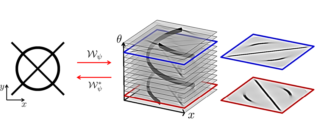
Refer to caption
Figure 3: Image processing via invertible orientation scores. Operators �\Phi on the invertible orientation score robustly relate to operators �\Upsilon on the image domain. Euclidean-invariance of �\Upsilon is obtained by left-invariance of �\Phi. Thus, we consider left-invariant (convection)-diffusion operators �=�t\Phi=\Phi_{t} with evolution time tt, which are generated by a quadratic form Q=QD,a​(𝒜∞,𝒜∈,𝒜∋)Q=Q^{\textbf{D},\textbf{a}}(\mathcall{A}_{1},\mathcall{A}_{2},\mathcall{A}_{3}) ( cf. ​Eq. ​(11)) on the left-invariant vector fields {𝒜⟩}\{\mathcall{A}_{i}\}, cf. ​Eq. ​(8). We show the relevance of left-invariance of 𝒜∈\mathcall{A}_{2} acting on an image of a circle (as in Figure 2) compared to action of the non-left-invariant derivative ∂y\partial_{y} on the same image.

2.2 Left-invariant Tangent Vectors and Vector Fields

The Euclidean motion group S​E​(2)SE(2) is a Lie group. Its tangent space at the unity element Te​(S​E​(2))T_{e}(SE(2)) is the corresponding Lie algebra and it is spanned by the basis {ex,ey,e�}\{\textbf{e}_{x},\textbf{e}_{y},\textbf{e}_{\theta}\}. Next we derive the left-invariant derivatives associated to ex,ey,e�\textbf{e}_{x},\textbf{e}_{y},\textbf{e}_{\theta}, respectively. A tangent vector Xe∈Te​(S​E​(2))X_{e}\in T_{e}(SE(2)) is tangent to a curve \gamma at unity element e=(0,0,0)e=(0,0,0). Left-multiplication of the curve \gamma with g∈S​E​(2)g\in SE(2) associates to each Xe∈Te​(S​E​(2))X_{e}\in T_{e}(SE(2)) a corresponding tangent vector Xg=(Lg)∗​Xe∈Tg​(S​E​(2))X_{g}=(L_{g})_{*}X_{e}\in T_{g}(SE(2)):

{e�​(g),e�​(g),e�​(g)}\displaystyle\{\textbf{e}_{\xi}(g),\textbf{e}_{\eta}(g),\textbf{e}_{\theta}(g)\} ={(Lg)∗​ex,(Lg)∗​ey,(Lg)∗​e�}\displaystyle=\{(L_{g})_{*}\textbf{e}_{x},(L_{g})_{*}\textbf{e}_{y},(L_{g})_{*}\textbf{e}_{\theta}\} (6)
={cos⁡�​ex+sin⁡�​ey,−sin⁡�​ex+cos⁡�​ey,e�},\displaystyle=\{\cos\theta\textbf{e}_{x}\!+\!\sin\theta\textbf{e}_{y},-\sin\theta\textbf{e}_{x}\!+\!\cos\theta\textbf{e}_{y},\textbf{e}_{\theta}\},

where (Lg)∗(L_{g})_{*} denotes the pushforward of left-multiplication Lg​h=g​hL_{g}h=gh, and where we introduce the local coordinates �:=x​cos⁡�+y​sin⁡�\xi:=x\cos\theta+y\sin\theta and �:=−x​sin⁡�+y​cos⁡�\eta:=-x\sin\theta+y\cos\theta. As the vector fields can also be considered as differential operators on locally defined smooth functions [5], we replace ei\textbf{e}_{i} by using ∂i\partial_{i}, i=�,�,�i=\xi,\eta,\theta, yielding the general form for a left-invariant vectorfield

Xg(U)=(c�(cos�∂x+sin�∂y)+c�(−sin�∂x+cos�∂y)+c�∂�)U, for all c�,c�,c�∈R.\displaystyle X_{g}(U)=(c^{\xi}(\cos\theta\partial_{x}+\sin\theta\partial_{y})+c^{\eta}(-\sin\theta\partial_{x}+\cos\theta\partial_{y})+c^{\theta}\partial_{\theta})U,\textit{ for all }c^{\xi},c^{\eta},c^{\theta}\in\mdmathbb{R}. (7)

Throughout this article, we shall rely on the following notation for left-invariant vector fields

{𝒜∞,𝒜∈,𝒜∋}:={∂�,∂�,∂�}={cos�∂§+sin�∂†,−sin�∂§+cos�∂†,∂�},\{\mathcall{A}_{1},\mathcall{A}_{2},\mathcall{A}_{3}\}:=\{\partial_{\xi},\partial_{\eta},\partial_{\theta}\}=\{\cos\theta\partial_{x}+\sin\theta\partial_{y},-\sin\theta\partial_{x}+\cos\theta\partial_{y},\partial_{\theta}\}, (8)

which is the frame of left-invariant derivatives acting on S​E​(2)SE(2), the domain of the orientation scores.

3 The PDE’s of Interest

3.1 Diffusions and Convection-Diffusions on S​E​(2)SE(2)

A diffusion process on Rn\mdmathbb{R}^{n} with a square integrable input image f:Rn⟼Rf:\mdmathbb{R}^{n}\longmapsto\mdmathbb{R} is given by

{∂tu⁡(x,t)=Ï⋅D​Ï​u​(x,t)x∈Rn,t≥0,u⁡(x,0)=f⁡(x).\displaystyle\left\{\begin{aligned} &\partial_{t}u(\textbf{x},t)=\triangledown\cdot\textbf{D}\triangledown u(\textbf{x},t)\qquad\textbf{x}\in\mdmathbb{R}^{n},t\geq 0,\\ &u(\textbf{x},0)=f(\textbf{x}).\\ \end{aligned}\right. (9)

Here, the Ï\triangledown operator is defined based on the spatial coordinates with Ï=(∂x1,…,∂xn)\triangledown=(\partial_{x_{1}},...,\partial_{x_{n}}), and the constant diffusion tensor D is a positive definite matrix of size n×nn\times n. Similarly, the left-invariant diffusion equation on S​E​(2)SE(2) is given by:

{∂tW⁡(g,t)=(∂�∂�∂�)​(D�​�D�​�D�​�D�​�D�​�D�​�D�​�D�​�D�​�)​(∂�∂�∂�)​W​(g,t),W⁡(g,t=0)=U0​(g),\displaystyle\left\{\begin{aligned} \partial_{t}W(g,t)&=\left(\begin{array}[]{ccc}\partial_{\xi}&\partial_{\eta}&\partial_{\theta}\end{array}\right)\left(\begin{array}[]{ccc}D_{\xi\xi}&D_{\xi\eta}&D_{\xi\theta}\\ D_{\eta\xi}&D_{\eta\eta}&D_{\eta\theta}\\ D_{\theta\xi}&D_{\theta\eta}&D_{\theta\theta}\\ \end{array}\right)\left(\begin{array}[]{ccc}\partial_{\xi}\\ \partial_{\eta}\\ \partial_{\theta}\end{array}\right)W(g,t),\\ W(g,t=0)&=U^{0}(g),\\ \end{aligned}\right. (10)

where as a default the initial condition is usually chosen as the orientation score of image f∈L2​(R2)f\in\mdmathbb{L}_{2}(\mdmathbb{R}^{2}), U0=Uf=𝒲{U^{0}=U_{f}=\mathcall{W}f. From the general theory for left-invariant scale spaces [23], the quadratic form of the convection-diffusion generator is given by

QD,a(𝒜∞,𝒜∈,𝒜∋)=∑⟩=∞∋(−⊣⟩𝒜⟩+∑|=∞∋𝒟⟩|𝒜⟩𝒜|),\displaystyle Q^{\textbf{D},\textbf{a}}(\mathcall{A}_{1},\mathcall{A}_{2},\mathcall{A}_{3})=\sum_{i=1}^{3}\left(-a_{i}\mathcall{A}_{i}+\sum_{j=1}^{3}D_{ij}\mathcall{A}_{i}\mathcall{A}_{j}\right), (11)
ai,Di​j∈R,D:=[Di​j]≥0,DT=D,\displaystyle a_{i},D_{ij}\in\mdmathbb{R},\textbf{D}:=[D_{ij}]\geq 0,\textbf{D}^{T}=\textbf{D},

where the first order part takes care of the convection process, moving along the exponential curves t⟼g⋅e​x​p​(t⁡(∑i=13ai​Ai))t\longmapsto g\cdot exp(t(\sum_{i=1}^{3}a_{i}A_{i})) over time with g∈S​E​(2)g\in SE(2), and the second order part specifies the diffusion in the following left-invariant evolutions

{∂tW=QD,a​(𝒜∞,𝒜∈,𝒜∋)​𝒲,W(⋅,t=0)=U0(⋅).\displaystyle\left\{\begin{aligned} &\partial_{t}W=Q^{\textbf{D},\textbf{a}}(\mathcall{A}_{1},\mathcall{A}_{2},\mathcall{A}_{3})W,\\ &W(\cdot,t=0)=U^{0}(\cdot).\\ \end{aligned}\right. (12)

In case of linear diffusion, the positive definite diffusion matrix D is constant. Then we obtain the solution of the left-invariant diffusion equation via a S​E​(2)SE(2)-convolution with the Green’s function KtD,a:S​E​(2)→R+K_{t}^{\textbf{D},\textbf{a}}:SE(2)\rightarrow\mdmathbb{R}^{+} and the initial condition U0:S​E​(2)→CU^{0}:SE(2)\to\mdmathbb{C}:

W⁡(g,t)=(KtD,a∗S​E​(2)U0)​(g)\displaystyle W(g,t)=(K_{t}^{\textbf{D},\textbf{a}}\ast_{SE(2)}U^{0})(g) =∫S​E​(2)KtD,a​(h−1​g)​U0​(h)​𝑑h\displaystyle=\int\limits_{SE(2)}K_{t}^{\textbf{D},\textbf{a}}(h^{-1}g)U^{0}(h)\,{\rm d}h (13)
=∫R2∫−��KtD,a​(R�′−1​(x−x′),�−�′)​U0​(x′,�′)​d​�′​d​x′,\displaystyle=\int\limits_{\mdmathbb{R}^{2}}\int\limits_{-\pi}^{\pi}K_{t}^{\textbf{D},\textbf{a}}(\textbf{R}_{\theta^{\prime}}^{-1}(\textbf{x}-\textbf{x}^{\prime}),\theta-\theta^{\prime})U^{0}(\textbf{x}^{\prime},\theta^{\prime})\,{\rm d}\theta^{\prime}{\rm d}\textbf{x}^{\prime},

for all g=(x,�)∈S​E​(2)g=(\textbf{x},\theta)\in SE(2). This can symbolically be written as W⁡(⋅,t)=et​QD,a​(𝒜∞,𝒜∈,𝒜∋)​U0​(⋅)W(\cdot,t)=e^{tQ^{\textbf{D},\textbf{a}}(\mathcall{A}_{1},\mathcall{A}_{2},\mathcall{A}_{3})}U^{0}(\cdot). In this time dependent diffusion we have to set a fixed time t>0t>0. In the subsequent sections we consider time integration while imposing a negatively exponential distribution T∼N​E​(�)T\sim NE(\alpha), i.e. P⁡(T=t)=�​e−�​tP(T=t)=\alpha e^{-\alpha t}. We choose this distribution since it is the only continuous memoryless distribution, and in order to ensure that the underlying stochastic process is Markovian, traveling time must be memoryless.

There are two specific cases of interest:

  • •

    Contour enhancement, where a=0\textbf{a}=\textbf{0} and D is symmetric positive semi-definite such that the Hörmander condition is satisfied. This includes both elliptic diffusion D>0\textbf{D}>0 and hypo-elliptic diffusion in which case we have D≥0\textbf{D}\geq 0 in such a way that Hörmander’s condition [37] is still satisfied. In the linear case we shall be mainly concerned with the hypo-elliptic case D=diag​{D11,0,D33}\textbf{D}=\textrm{diag}\{D_{11},0,D_{33}\},

  • •

    Contour completion, where a=(1,0,0)\textbf{a}=(1,0,0) and D=diag​{0,0,D33}\textbf{D}=\textrm{diag}\{0,0,D_{33}\} with D33>0D_{33}>0.

Several new exact representations for the (resolvent) Green’s functions in S​E​(2)SE(2) were derived by Duits et al. [25, 29, 27, 28, 56] in the spatial Fourier domain, as explicit formulas were still missing, see e.g. [46]. This includes the Fourier series representations, studied independently in [12], but also includes a series of rapidly decaying terms and explicit representations obtained by computing the latter series representations explicitly via the Floquet theorem, producing explicit formulas involving only 4 Mathieu functions. The works in [25, 29] relied to a large extend on distribution theory to derive these explicit formulas. Here we deal with the general case with D≥0D\geq 0 and a∈R3\textbf{a}\in\mdmathbb{R}^{3} (as long as Hörmander’s condition [37] is satisfied) and we stress the analogy between the contour completion and contour enhancement case in the appropriate general setting (for the resolvent PDE, for the (convection)-diffusion PDE, and for fundamental solution PDE). Instead of relying on distribution theory [29, 25], we obtain the general solutions more directly via Sturm-Liouville theory.

Furthermore, in Section 6 we include, for the first time, numerical comparisons of various numerical approaches to the exact solutions. The outcome of which, is underpinned by a strong convergence theorem that we will present in Theorem 5.4.

On top of this, in Appendix B, we shall present new asymptotic expansions around the origin that allow us to analyze the order of the singularity at the origin of the resolvent kernels. From these asymptotic expansions we deduce that the singularities in the resolvent kernels (and fundamental solutions) are quite severely. In fact, the better the equations are numerically approximated, the weaker the completion and enhancement properties of the kernels.

To overcome this severe discrepancy between the mathematical PDE theory and the practical requirements, we propose time-integration via Gamma distributions (beyond the negative exponential distribution case). Mathematically, as we will prove in Subsection 3.3, this newly proposed time integration both reduces the singularities, and maintains the formal PDE theory. In fact using a Gamma distribution coincides with iteration the resolvents, with an iteration depth kk equal to the squared mean divided by the variance of the Gamma distribution.

We will also show practical experiments that demonstrate the advantage of using the Gamma-distributions: we can control and amplify the infilling property ("the spread of ink") of the PDE’s.

3.2 The Resolvent Equation

Traveling time of a memoryless random walker in S​E​(2)SE(2) is negatively exponential distributed, i.e.

p⁡(T=t)=�​e−�​t,t≥0,\displaystyle p(T=t)=\alpha e^{-\alpha t},t\geq 0, (14)

with the expected life time E⁡(T)=1�E(T)=\frac{1}{\alpha}. Then the resolvent kernel is obtained by integrating Green’s function KtD,a:S​E​(2)→R+K_{t}^{\textbf{D},\textbf{a}}:SE(2)\rightarrow\mdmathbb{R}^{+} over the time distribution, i.e.

R�D,a\displaystyle R_{\alpha}^{\textbf{D},\textbf{a}} =�​∫0∞KtD,a​e−�​t​dt=�​∫0∞et​Q​�e​e−�​t​dt=−�​(Q−�​I)−1​�e,\displaystyle=\alpha\int_{0}^{\infty}K_{t}^{\textbf{D},\textbf{a}}e^{-\alpha t}dt=\alpha\int_{0}^{\infty}e^{tQ}\delta_{e}e^{-\alpha t}dt=-\alpha(Q-\alpha I)^{-1}\delta_{e},

where we use short notation Q=QD,a​(𝒜∞,𝒜∈,𝒜∋)Q=Q^{\textbf{D},\textbf{a}}(\mathcall{A}_{1},\mathcall{A}_{2},\mathcall{A}_{3}). Via this resolvent kernel, one gets the probability density P�​(g)P_{\alpha}(g) of finding a random walker at location g∈S​E​(2)g\in SE(2) regardless its traveling time, given that it has departed from distribution U:S​E​(2)→R+U:SE(2)\to\mdmathbb{R}^{+}:

P�(g)=(R�D,a∗S​E​(2)U)(g)=−�(QD,a(𝒜∞,𝒜∈,𝒜∋)−�ℐ)−∞𝒰(}),\displaystyle P_{\alpha}(g)=(R_{\alpha}^{\textbf{D},\textbf{a}}\ast_{SE(2)}U)(g)=-\alpha(Q^{\textbf{D},\textbf{a}}(\mathcall{A}_{1},\mathcall{A}_{2},\mathcall{A}_{3})-\alpha I)^{-1}U(g), (15)

which is the same as taking the Laplace transform of the left-invariant evolution equations  (12) over time. The resolvent equation can be written as

P�​(g)=�​∫0∞e−�​t​(et​Q​U0)​(g)​dt=�​((�​I−Q)−1​U)​(g).\displaystyle P_{\alpha}(g)=\alpha\int_{0}^{\infty}e^{-\alpha t}(e^{tQ}U^{0})(g)dt=\alpha((\alpha I-Q)^{-1}U)(g).

However, we do not want to go into the details of semigroup theory [57] and just included where (et​Q​U0)(e^{tQ}U^{0}) in short notation for the solution of Eq. (12). Resolvents can be used in completion fields[58, 25, 6]. Some resolvent kernels of the contour enhancement and completion process are given in Figure 4.

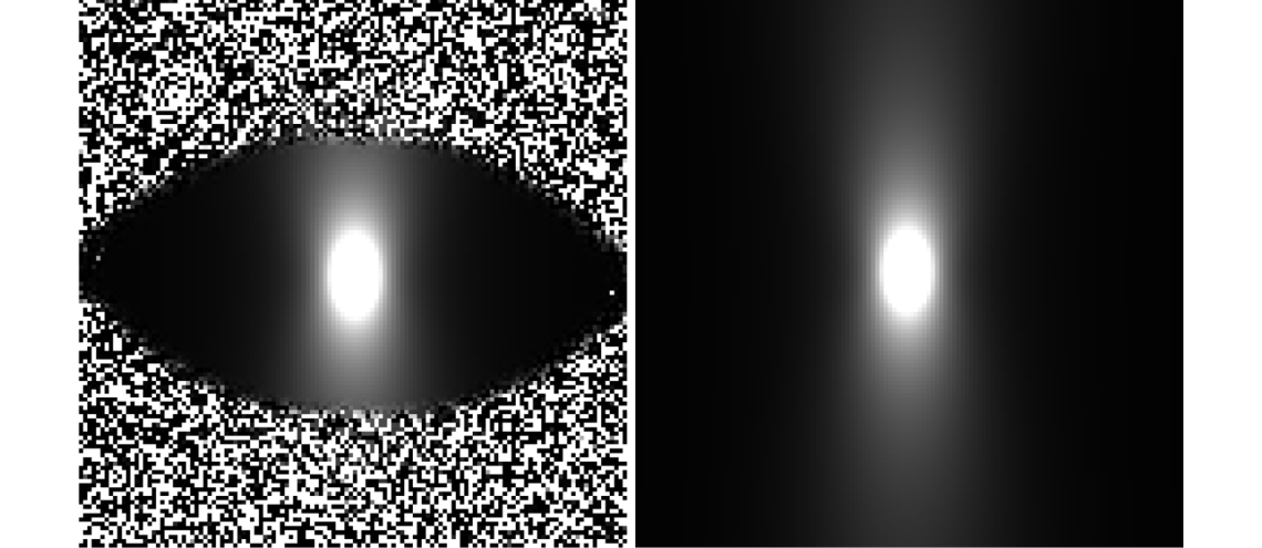
Refer to caption
Figure 4: Left: the x​yxy-marginal of the contour enhancement kernel R�D:=R�D,0R_{\alpha}^{\textbf{D}}:=R_{\alpha}^{\textbf{D},\textbf{0}} with parameters �=1100\alpha=\frac{1}{100}, D={1,0,0.08}\textbf{D}=\{1,0,0.08\}, numbers of orientations No=48N_{o}=48 and spatial dimensions Ns=128N_{s}=128. Right: the x​yxy-marginal of the contour completion kernel R�D,aR_{\alpha}^{\textbf{D},\textbf{a}} with parameters �=1100\alpha=\frac{1}{100}, a=(1,0,0)\textbf{a}=(1,0,0), D={0,0,0.08}\textbf{D}=\{0,0,0.08\}, No=72N_{o}=72 and Ns=192N_{s}=192.

3.3 Improved Kernels via Iteration of Resolvent Operators

The kernels of the resolvent operators suffer from singularities at the origin. Especially for contour completion, this is cumbersome from the application point of view, since here the better one approximates Mumford’s direction process and its inherent singularity in the Green’s function, the less “ink” is spread in the areas with missing and interrupted contours. To overcome this problem we extend the temporal negatively exponential distribution in our line enhancement/completion models by a 1-parameter family of Gamma-distributions.

As a sum T=T1+…+TkT=T_{1}+\ldots+T_{k} of linearly independent negatively exponential time variables is Gamma distributed P⁡(T=t)=�k​tk−1(k−1)!​e−�​tP(T=t)=\frac{\alpha^{k}t^{k-1}}{(k-1)!}e^{-\alpha t}, the time integrated process is now obtained by a kk-fold resolvent operator. While keeping the expectation of the Gamma distribution fixed by E⁡(T)=k/�E(T)=k/\alpha, increasing of kk will induce more mass transport away from t=0t=0 towards the void areas of interrupted contours. For k≥3k\geq 3 the corresponding Green’s function of the kk-step approach even no longer suffers from a singularity at the origin. This procedure is summarized in the following theorem and applied in Figure 5.

Theorem 3.1.

A concatenation of kk subsequent, independent time-integrated memoryless stochastic process for contour enhancement(/completion) with expected traveling time �−1\alpha^{-1}, corresponds to a time-integrated contour enhancement(/completion) process with a Gamma distributed traveling time T=T1+…+TkT=T_{1}+\ldots+T_{k} with

P(Ti=t)=�e−�​t, for i=1,…,k,P⁡(T=t)=�⁡(t,k,�):=�k​tk−1�⁡(k)​e−�​t.\begin{array}[]{l}P(T_{i}=t)=\alpha e^{-\alpha t},\textrm{ for }i=1,\ldots,k,\\ P(T=t)=\Gamma(t;k,\alpha):=\frac{\alpha^{k}t^{k-1}}{\Gamma(k)}e^{-\alpha t}.\end{array} (16)

The probability density kernel of this stochastic process is given by

R�,kD,a=R�D,a∗S​E​(2)(k−1)R�D,a=�k(QD,a(𝒜¯)−�ℐ)−⁣∥�⌉,R_{\alpha,k}^{\textbf{D},\textbf{a}}=R_{\alpha}^{\textbf{D},\textbf{a}}*^{(k-1)}_{SE(2)}R_{\alpha}^{\textbf{D},\textbf{a}}=\alpha^{k}(Q^{\textbf{D},\textbf{a}}(\underline{\mathcall{A}})-\alpha I)^{-k}\delta_{e}, (17)

For the linear, hypo-elliptic, contour enhancement case (i.e. D=diag​{D11,0,D33}\textbf{D}=\textrm{diag}\{D_{11},0,D_{33}\} and a=0\textbf{a}=\textbf{0}) the kernels admit the following asymptotical formula for |g|<<1:|g|<<1:

R�,k​(g)=∫0∞�k​tk−1​e−�​t(k−1)!​e−C2​|g|24​t4​�​D11​D33​t2​𝑑t=�k(k−1)!​4​�​D11​D33​∫0∞tk−3​e−C2​|g|24​t−�​t​𝑑t=21−k�​D11​D33​(k−1)!�k||g|C|k−2𝒦(∈−∥,|}|𝒞�),\begin{array}[]{ll}R_{\alpha,k}(g)&=\int\limits_{0}^{\infty}\frac{\alpha^{k}t^{k-1}e^{-\alpha t}}{(k-1)!}\frac{e^{-C^{2}\frac{|g|^{2}}{4t}}}{4\pi D_{11}D_{33}t^{2}}{\rm d}t=\frac{\alpha^{k}}{(k-1)!4\pi D_{11}D_{33}}\int\limits_{0}^{\infty}t^{k-3}e^{-C^{2}\frac{|g|^{2}}{4t}-\alpha t}\,{\rm d}t\\ &=\frac{2^{1-k}}{\pi D_{11}D_{33}(k-1)!}\alpha^{k}||g|C|^{k-2}\;\mathcall{K}(2-k,|g|C\sqrt{\alpha}),\end{array} (18)

where 𝒦⁡(\,‡)\mathcall{K}(n,z) denotes the modified Bessel function of the 2nd kind, and with C∈[2−1,24]C\in[2^{-1},\sqrt[4]{2}] and with

|g|=|ec1𝒜∞+⌋∈𝒜∈+⌋∋𝒜∋|=(|c1|2D11+|c3|2D33)2+|c2|2D11​D33|g|=\left|e^{c^{1}\mathcall{A}_{1}+c^{2}\mathcall{A}_{2}+c^{3}\mathcall{A}_{3}}\right|=\sqrt{\left(\frac{|c^{1}|^{2}}{D_{11}}+\frac{|c^{3}|^{2}}{D_{33}}\right)^{2}+\frac{|c^{2}|^{2}}{D_{11}D_{33}}} (19)

with c1=�​(y−�)2​(1−cos⁡�)c^{1}=\frac{\theta(y-\eta)}{2(1-\cos\theta)}, c2=�​(�−x)2​(1−cos⁡�)c^{2}=\frac{\theta(\xi-x)}{2(1-\cos\theta)}, c3=�c^{3}=\theta if �≠0\theta\neq 0 and (c1,c2,c3)=(x,y,0)(c^{1},c^{2},c^{3})=(x,y,0) if �=0\theta=0.

Proof We consider a random traveling time T=∑i=1nTiT=\sum_{i=1}^{n}T_{i} in an nn-step approach random process GT=∑i=1NGTiG_{T}=\sum_{i=1}^{N}G_{T_{i}} on S​E​(2)SE(2), with GTiG_{T_{i}} independent random random walks whose Fokker-Planck equations are given by (12), and with independent traveling times Ti∼N​E​(�)T_{i}\sim NE(\alpha) (i.e. P⁡(Ti=t)=f⁡(t):=�​e−�​tP(T_{i}=t)=f(t):=\alpha e^{-\alpha t}). Then for k≥2k\geq 2 we have T∼f∗R+k−1f=�⁡(⋅,k,�)T\sim f*_{\mdmathbb{R}^{+}}^{k-1}f=\Gamma(\cdot;k,\alpha), (with f∗R+g⁡(t)=∫0tf⁡(�)​g​(t−�)​𝑑�f*_{\mdmathbb{R}^{+}}g(t)=\int_{0}^{t}f(\tau)g(t-\tau)\,{\rm d}\tau), which follows by consideration of the characteristic function and application of Laplace transform ℒ\mathcall{L}.

We have �k​(Q−�​I)−k=(�​(Q−�​I)−1)k\alpha^{k}(Q-\alpha I)^{-k}=(\alpha(Q-\alpha I)^{-1})^{k}, and for k=2k=2 we have identity

R�,k=2D,a​(x,�)=∫0∞p⁡(GT=(x,�)|T=t,G0=e)⋅p⁡(T=t)​𝑑t=∫0∞p(GT=(x,�)|T=T1+T2=t,G0=e)⋅p(T1+T2=t)dt=∫0∞∫0tp⁡(GT1+T2=(x,�)|T1=t−s,T2=s,G0=e)⋅p⁡(T1=t−s)​p​(T2=s)​𝑑s​𝑑t=�2ℒ(⊔↦∫′⊔(𝒦⊔−∫D,a∗𝒮ℰ⁡(∈)𝒦∫D,a∗𝒮ℰ⁡(∈)�⌉)(x,�)⌈∫)(�)=�2ℒ(⊔↦∫′⊔(𝒦⊔−∫D,a∗𝒮ℰ⁡(∈)𝒦∫D,a)(x,�)⌈∫)(�)=�2(ℒ(⊔↦𝒦⊔D,a(⋅))(�)∗𝒮ℰ⁡(∈)ℒ(⊔↦𝒦⊔D,a(⋅))(�))(x,�)=(R�,k=1D,a∗S​E​(2)R�,k=1D,a)(x,�).\begin{array}[]{l}R_{\alpha,k=2}^{\textbf{D},\textbf{a}}(\textbf{x},\theta)=\int\limits_{0}^{\infty}p(G_{T}=(\textbf{x},\theta)|T=t,G_{0}=e)\cdot p(T=t)\,{\rm d}t\\ =\int\limits_{0}^{\infty}p(G_{T}=(\textbf{x},\theta)\;|\;T=T_{1}+T_{2}=t,G_{0}=e)\cdot p(T_{1}+T_{2}=t)\,{\rm d}t\\ =\int\limits_{0}^{\infty}\int\limits_{0}^{t}p(G_{T_{1}+T_{2}}=(\textbf{x},\theta)\;|\;T_{1}=t-s,T_{2}=s,G_{0}=e)\cdot p(T_{1}=t-s)\;p(T_{2}=s)\,{\rm d}s{\rm d}t\\ =\alpha^{2}\,\mathcall{L}\left(t\mapsto\int\limits_{0}^{t}(K_{t-s}^{\textbf{D},\textbf{a}}*_{SE(2)}K_{s}^{\textbf{D},\textbf{a}}*_{SE(2)}\delta_{e})(\textbf{x},\theta){\rm d}s\right)(\alpha)\\ =\alpha^{2}\,\mathcall{L}\left(t\mapsto\int\limits_{0}^{t}(K_{t-s}^{\textbf{D},\textbf{a}}*_{SE(2)}K_{s}^{\textbf{D},\textbf{a}})(\textbf{x},\theta){\rm d}s\right)(\alpha)\\ =\alpha^{2}\,\left(\mathcall{L}\left(t\mapsto K_{t}^{\textbf{D},\textbf{a}}(\cdot)\right)(\alpha)*_{SE(2)}\mathcall{L}\left(t\mapsto K_{t}^{\textbf{D},\textbf{a}}(\cdot)\right)(\alpha)\right)(\textbf{x},\theta)=(R_{\alpha,k=1}^{\textbf{D},\textbf{a}}*_{SE(2)}R_{\alpha,k=1}^{\textbf{D},\textbf{a}})(\textbf{x},\theta).\end{array}

Thereby main result Eq. ​(17) follows by induction.

Result (18) follows by direct computation and application of the theory of weighted sub-coercive operators on Lie groups [30] to the S​E​(2)SE(2) case. We have filtration 𝔤0:=span​{𝒜∞,𝒜∋}\gothic{g}_{0}:=\textrm{span}\{\mathcall{A}_{1},\mathcall{A}_{3}\}, and 𝔤1=[𝔤0,𝔤0]=span​{𝒜∞,𝒜∈,𝒜∋}=ℒ⁡(𝒮ℰ⁡(∈))\gothic{g}_{1}=[\gothic{g}_{0},\gothic{g}_{0}]=\textrm{span}\{\mathcall{A}_{1},\mathcall{A}_{2},\mathcall{A}_{3}\}=\mathcall{L}(SE(2)), so w1=1w_{1}=1, w3=1w_{3}=1 and w2=2w_{2}=2 and computation of the logarithmic map on S​E​(2)SE(2), g=e∑i=13ci​Ai⇔∑i=13ci​Ai=log⁡gg=e^{\sum_{i=1}^{3}c^{i}A_{i}}\Leftrightarrow\sum_{i=1}^{3}c^{i}A_{i}=\log g, yields a non-smooth logarithmic squared modulus locally equivalent to smooth |g|2|g|^{2} given by (19), see [25, ch:5.4,eq.5.28]. ƒ\hfill\square

We have the following asymptotical formula for 𝒦⁡(\,‡)\mathcall{K}(n,z):

𝒦(\,‡)≈{−log(‡/∈)−ℰ𝒰ℒif \=′∞∈(|\|−∞)!(‡∈)−|\| for ′<‡<<∞,\mathcall{K}(n,z)\approx\left\{\begin{array}[]{ll}-\log(z/2)-{}_{EUL}&\textrm{if }n=0\\ \frac{1}{2}(|n|-1)!\left(\frac{z}{2}\right)^{-|n|}\end{array}\right.\textrm{ for }0<z<\!<\!1,

with Euler’s constant EUL, and thereby Eq. (18) implies the following result:

Corollary 3.2.

If k=1k=1 then R�,kD​(g)≡O⁡(|g|−2)R_{\alpha,k}^{\textbf{D}}(g)\equiv O(|g|^{-2}). If k=2k=2 then R�,kD​(g)≡O⁡(log⁡|g|−1)R_{\alpha,k}^{\textbf{D}}(g)\equiv O(\log|g|^{-1}). If k≥3k\geq 3 then R�,kD​(g)≡O⁡(1)R_{\alpha,k}^{\textbf{D}}(g)\equiv O(1) and the kernel has no singularity.

Remark 3.3.

As this approach also naturally extends to positive (non-integer) fractional powers k∈Q,k≥0k\in\mdmathbb{Q},k\geq 0 of the resolvent operator we wrote �⁡(k)\Gamma(k) instead of (k−1)!(k-1)! in Eq. ​(16). The recursion depth kk equals (E⁡(T))2/V​a​r​(T)(E(T))^{2}/Var(T), since the variance of TT equals V​a​r​(T)=k/�2Var(T)=k/\alpha^{2}.

In Figure 5, we show that increase of kk (while fixing E⁡(T)=k/�E(T)=k/\alpha) allows for better propagation of ink towards the completion areas. The same concept applies to the contour enhancement process. Here we change time integration (using the stochastic approach outlined in Section 4.4) in Eq. ​(16) rather than iterating the resolvents in Eq. ​(17) for better accuracy.

Refer to caption
Figure 5: Illustration of Theorem 3.1 and Corollary 3.2, via the stochastic implementation for the kk-step contour completion process (T=∑i=1kTiT=\sum_{i=1}^{k}T_{i}) explained in Subsection 4.4. We have depicted the (2D marginals) of 3D completion fields [58] now generalized to 𝒞(§,†,�):=((𝒬−(�∥)ℐ)−⁣∥�}′)(§,†,�)⋅((𝒬∗−(�∥)ℐ)−⁣∥�}∞)(§,†,�)\mathcall{C}(x,y,\theta):=((Q-(\alpha k)I)^{-k}\delta_{g_{0}})(x,y,\theta)\cdot((Q^{*}-(\alpha k)I)^{-k}\delta_{g_{1}})(x,y,\theta), with Q=−𝒜∞+𝒟∋⁣∋​𝒜∋∈Q=-\mathcall{A}_{1}+D_{33}\mathcall{A}_{3}^{2} and with g0=(x0,�6)g_{0}=(\textbf{x}_{0},\frac{\pi}{6}) and g1=(x1,−�6)g_{1}=(\textbf{x}_{1},-\frac{\pi}{6}), �=0.1\alpha=0.1, D33=0.1D_{33}=0.1, via a rough resolution (on a 200×200×32200\times 200\times 32-grid) and a finer resolution (on a 400×400×64400\times 400\times 64-grid). Image intensities have been scaled to full range. The resolvent process k=1k=1 suffers from: "the better the approximation, the less relative infilling in the completion" (cf. left column). The singularities at g0g_{0} and g1g_{1} vanish at k=3k=3. A reasonable compromise is found at k=2k=2 where infilling is stronger, and where the modes (i.e. curves \gamma with 𝒜∈𝒞( )=𝒜∋𝒞( )=′\mathcall{A}_{2}\mathcall{C}(\gamma)=\mathcall{A}_{3}C(\gamma)=0, cf. [10, App. A],[29]) are easy to detect.

3.4 Fundamental Solutions

The fundamental solution SD,a:S​E​(2)→R+S^{\textbf{D},\textbf{a}}:SE(2)\to\mdmathbb{R}^{+} associated to generator QD,a​(𝒜∞,𝒜∈,𝒜∋)Q^{\textbf{D},\textbf{a}}(\mathcall{A}_{1},\mathcall{A}_{2},\mathcall{A}_{3}) solves

QD,a(𝒜∞,𝒜∈,𝒜∋)𝒮D,a=−�⌉,Q^{\textbf{D},\textbf{a}}(\mathcall{A}_{1},\mathcall{A}_{2},\mathcall{A}_{3})\;S^{\textbf{D},\textbf{a}}=-\delta_{e}\ , (20)

and is given by

SD,a​(x,y,�)\displaystyle S^{\textbf{D},\textbf{a}}(x,y,\theta) =∫0∞KtD,a(x,y,�)dt=(−(QD,a(𝒜∞,𝒜∈,𝒜∋))−∞�⌉)(x,y,�)\displaystyle=\int\limits_{0}^{\infty}K_{t}^{\textbf{D},\textbf{a}}(x,y,\theta)\,{\rm d}t=\left(-(Q^{\textbf{D},\textbf{a}}(\mathcall{A}_{1},\mathcall{A}_{2},\mathcall{A}_{3}))^{-1}\delta_{e}\right)(x,y,\theta) (21)
=lim�↓0(−�​(QD,a​(𝒜∞,𝒜∈,𝒜∋)−�​ℐ)−∞�​�e)​(x,y,�)=lim�↓0R�D,a​(x,y,�)�.\displaystyle=\lim_{\alpha\downarrow 0}\left(\frac{-\alpha(Q^{\textbf{D},\textbf{a}}(\mathcall{A}_{1},\mathcall{A}_{2},\mathcall{A}_{3})-\alpha I)^{-1}}{\alpha}\delta_{e}\right)(x,y,\theta)=\lim_{\alpha\downarrow 0}\frac{R_{\alpha}^{\textbf{D},\textbf{a}}(x,y,\theta)}{\alpha}.

There exist many intriguing relations [26, 14] between fundamental solutions of hypo-elliptic diffusions and left-invariant metrics on S​E​(2)SE(2), which make these solutions interesting. Furthermore, fundamental solutions on the nilpotent approximation (S​E​(2))0(SE(2))_{0} take a relatively simple explicit form [35, 25]. However, by Eq. (21) these fundamental solutions suffer from some practical drawbacks: they are not probability kernels, in fact they are not even L1\mdmathbb{L}_{1}-normalizable, and they suffer from poles in both spatial and Fourier domain. Nevertheless, they are interesting to study for the limiting case �↓0\alpha\downarrow 0 and they have been suggested in cortical modeling [9, 8].

3.5 The Underlying Probability Theory

In this section we provide an overview of the underlying probability theory belonging to our PDE’s of interest, given by Eq. (12), (15) and (20).

We obtain the contour enhancement case by setting D=diag​{D11,0,D33}\textbf{D}=\textrm{diag}\{D_{11},0,D_{33}\} and a=0\textbf{a}=\textbf{0}. Then, by application of Eq. (8), Eq. (12) becomes the forward Kolmogorov equation

{∂tW(g,t)=(D11∂�2+D33∂�2)W(g,t),W⁡(g,t=0)=U⁡(g)\left\{\begin{aligned} &\partial_{t}W(g,t)=(D_{11}\partial_{\xi}^{2}+D_{33}\partial_{\theta}^{2})W(g,t),\\ &W(g,t=0)=U(g)\\ \end{aligned}\right. (22)

of the following stochastic process for contour enhancement:

{X​(t)=X​(0)+2​D11​"�​∫0t(cos⁡�​(�)​ex+sin⁡�​(�)​ey)​12​�​d��(t)=�(0)+t2​D33"�,"�,"�𝑠𝒩(′,∞)\left\{\begin{aligned} &\textbf{X}(t)=\textbf{X}(0)+\sqrt{2D_{11}}\varepsilon_{\xi}\int^{t}_{0}(\cos\Theta(\tau)\textbf{e}_{x}+\sin\Theta(\tau)\textbf{e}_{y})\frac{1}{2\sqrt{\tau}}\,{\rm d}\tau\\ &\Theta(t)=\Theta(0)+\sqrt{t}\sqrt{2D_{33}}\varepsilon_{\theta},\qquad\varepsilon_{\xi},\varepsilon_{\theta}\thicksim\mathcall{N}(0,1)\\ \end{aligned}\right. (23)

For contour completion, we must set the diffusion matrix D=diag​{0,0,D33}\textbf{D}=\textrm{diag}\{0,0,D_{33}\} and convection vector a=(1,0,0)\textbf{a}=(1,0,0). In this case Eq. (12) takes the form

{∂tW(g,t)=(∂�+D33∂�2)W(g,t),g∈SE(2),t>0,W⁡(g,t=0)=U⁡(g).\left\{\begin{aligned} &\partial_{t}W(g,t)=(\partial_{\xi}+D_{33}\partial_{\theta}^{2})W(g,t),\qquad g\in SE(2),t>0,\\ &W(g,t=0)=U(g).\\ \end{aligned}\right. (24)

This is the Kolmogorov equation of Mumford’s direction process [46]

{X​(t)=X⁡(t)​ex+Y⁡(t)​ey=X​(0)+∫0tcos⁡�​(�)​ex+sin⁡�⁡(�)​ey​d��(t)=�(0)+t2​D33"�,"�𝑠𝒩(′,∞)\left\{\begin{aligned} &\textbf{X}(t)=X(t)\textbf{e}_{x}+Y(t)\textbf{e}_{y}=\textbf{X}(0)+\int^{t}_{0}\cos\Theta(\tau)\textbf{e}_{x}+\sin\Theta(\tau)\textbf{e}_{y}\,{\rm d}\tau\\ &\Theta(t)=\Theta(0)+\sqrt{t}\sqrt{2D_{33}}\varepsilon_{\theta},\qquad\varepsilon_{\theta}\thicksim\mathcall{N}(0,1)\\ \end{aligned}\right. (25)
Remark 3.4.

As contour completion processes aim to reconstruct the missing parts of interrupted contours based on the contextual information of the data, a positive direction e�=cos⁡(�)​ex+sin⁡(�)​ey\textbf{e}_{\xi}=\cos(\theta)\textbf{e}_{x}+\sin(\theta)\textbf{e}_{y} in the spatial plane is given to a random walker. On the contrary, in contour enhancement processes a bi-directional movement of a random walker along ±e�\pm\textbf{e}_{\xi} is included for noise removal by anisotropic diffusion.

The general stochastic process on S​E​(2)SE(2) underlying Eq. (12) is :

{Gn+1:=(Xn+1,�n+1)=Gn+�​t​∑i∈Iai​ei|Gn+�​t​∑i∈I�i,n+1​∑j∈I�j​i​ej|Gn,G0=(X0,�0),\left\{\begin{array}[]{l}G_{n+1}:=(X_{n+1},\Theta_{n+1})=G_{n}+\Delta t\sum\limits_{i\in I}a_{i}\left.\textbf{e}_{i}\right|_{G_{n}}+\sqrt{\Delta t}\sum\limits_{i\in I}\epsilon_{i,n+1}\,\sum\limits_{j\in I}\sigma_{ji}\,\left.\textbf{e}_{j}\right|_{G_{n}},\\ G_{0}=(X_{0},\Theta_{0}),\end{array}\right. (26)

with I={1,2,3}I=\{1,2,3\} in the elliptic case and I={1,3}I=\{1,3\} in the hypo-elliptic case and where n=1,…,N−1n=1,\ldots,N-1, N∈NN\in\mdmathbb{N} denotes the number of steps with stepsize �​t>0\Delta t>0, �=2​D\sigma=\sqrt{2D} is the unique symmetric positive definite matrix such that �2=2​D\sigma^{2}=2D, {�i,n+1}i∈I,n=1,…,N−1\{\epsilon_{i,n+1}\}_{i\in I,n=1,\ldots,N-1} are independent normally distributed �i,n+1∼𝒩(′,∞)\epsilon_{i,n+1}\sim\mathcall{N}(0,1) and e1|Gn=(cos⁡�n,sin⁡�n,0)\left.\textbf{e}_{1}\right|_{G_{n}}=(\cos\Theta_{n},\sin\Theta_{n},0), e2|Gn=(−sin⁡�n,cos⁡�n,0)\left.\textbf{e}_{2}\right|_{G_{n}}=(-\sin\Theta_{n},\cos\Theta_{n},0), and e3|Gn=(0,0,1)\left.\textbf{e}_{3}\right|_{G_{n}}=(0,0,1). In case I={1,2,3}I=\{1,2,3\}, Eq. (26) boils down to:

(Xn+1Yn+1�n+1)=(XnYn�n)+�​t​R�n​(a1a2a3)+�​t​(R�n)T​�​R�n​(�1,n+1�2,n+1�3,n+1), with ​R�=(cos⁡�−sin⁡�0sin⁡�cos⁡�0001).\begin{array}[]{l}\begin{array}[]{l}\left(\begin{array}[]{c}X_{n+1}\\ Y_{n+1}\\ \Theta_{n+1}\end{array}\right)=\left(\begin{array}[]{c}X_{n}\\ Y_{n}\\ \Theta_{n}\end{array}\right)+\Delta t\,{\rm R}_{\Theta_{n}}\left(\begin{array}[]{c}a_{1}\\ a_{2}\\ a_{3}\end{array}\right)+\sqrt{\Delta t}\,({\rm R}_{\Theta_{n}})^{T}\,\sigma\,\rm{R}_{\Theta_{n}}\left(\begin{array}[]{c}\epsilon_{1,n+1}\\ \epsilon_{2,n+1}\\ \epsilon_{3,n+1}\end{array}\right),\\ \textrm{ with }{\rm R}_{\theta}=\left(\begin{array}[]{ccc}\cos\theta&-\sin\theta&0\\ \sin\theta&\cos\theta&0\\ 0&0&1\end{array}\right).\end{array}\end{array} (27)

See Figure 6 for random walks of the Brownian motion and the direction process in S​E​(2)SE(2).

Refer to caption
Figure 6: From left to right: Up row: 20 random walks of the direction process for contour completion in S​E​(2)=R2𝑜S1SE(2)=\mdmathbb{R}^{2}\rtimes S^{1} by Mumford [46] with a=(1,0,0)\textbf{a}=(1,0,0), D33=0.3D_{33}=0.3, time step △​t\triangle t=0.005 and 1000 steps. Bottom row: 20 random walks of the linear left-invariant stochastic processes for contour enhancement within S​E​(2)SE(2) with parameter settings D11=D33=0.5D_{11}=D_{33}=0.5 and D22=0D_{22}=0, time step △​t\triangle t=0.05 and 1000 steps.

4 Implementation

4.1 Left-invariant Differences

4.1.1 Left-invariant Finite Differences with B-Spline Interpolation

As explained in Section 2.1, our diffusions must be left-invariant. Therefore, a new grid template based on the left-invariant frame {e�,e�,e�}\{\textbf{e}_{\xi},\textbf{e}_{\eta},\textbf{e}_{\theta}\}, instead of the fixed frame {ex,ey,e�}\{\textbf{e}_{x},\textbf{e}_{y},\textbf{e}_{\theta}\}, need to be used in the finite difference methods.

Refer to caption
(a)
Figure 7: Illustration of the spatial part of the stencil of the numerical scheme. The horizontal and vertical dashed lines indicate the sampling grid, which is aligned with {ex,ey}\{\textbf{e}_{x},\textbf{e}_{y}\}. The black dots, which are aligned with the rotated left-invariant coordinate system {e�,e�}\{\textbf{e}_{\xi},\textbf{e}_{\eta}\} with �=m⋅�​�\theta=m\cdot\Delta\theta, where m∈{0,1,…,No−1}m\in\{0,1,...,N_{o}-1\} denotes the sampled orientation equidistantly sampled with distance �​�=2​�No\Delta\theta=\frac{2\pi}{N_{o}}.

To understand how left-invariant finite differences are implemented, see Figure 7, where 2nd order B-spline interpolation [55] is used to approximate off-grid samples. The main advantage of this left-invariant finite difference scheme is the improved rotation invariance compared to finite differences applied after expressing the PDE’s in fixed (x,y,�)(x,y,\theta)-coordinates, such as in [14, 32, 58]. This advantage is clearly demonstrated in [33, Fig. 10]. The drawback, however, is the low computational speed and a small amount of additional blurring caused by the interpolation scheme [32].

4.2 Left-invariant Finite Difference Approaches for Contour Enhancement and Completion

Eq. (22) of the contour enhancement process and Eq. (24) of the contour completion process show us respectively the Brownian motion and direction process of oriented particles moving in S​E​(2)≡R2𝑜S1SE(2)\equiv\mdmathbb{R}^{2}\rtimes S^{1}. Next we will provide and analyze finite difference schemes for both processes.

4.2.1 Explicit Scheme for Linear Contour Enhancement and Completion

We can represent the explicit numerical approximations of the contour enhancement process and contour completion process by using the generator QD,a​(𝒜∞,𝒜∈,𝒜∋)Q^{\textbf{D},\textbf{a}}(\mathcall{A}_{1},\mathcall{A}_{2},\mathcall{A}_{3}) in a general form, i.e. QD,a(𝒜∞,𝒜∈,𝒜∋)=(𝒟∞​∞𝒜∞∈+𝒟∋⁣∋𝒜∋∈)=(𝒟∞​∞∂�∈+𝒟∋⁣∋∂�∈)Q^{\textbf{D},\textbf{a}}(\mathcall{A}_{1},\mathcall{A}_{2},\mathcall{A}_{3})=(D_{11}\mathcall{A}_{1}^{2}+D_{33}\mathcall{A}_{3}^{2})=(D_{11}\partial_{\xi}^{2}+D_{33}\partial_{\theta}^{2}) for the diffusion process and QD,a(𝒜∞,𝒜∈,𝒜∋)=(∂�+𝒟∋⁣∋∂�∈)Q^{\textbf{D},\textbf{a}}(\mathcall{A}_{1},\mathcall{A}_{2},\mathcall{A}_{3})=(\partial_{\xi}+D_{33}\partial_{\theta}^{2}) for the convection-diffusion process, which yield the following forward Euler discretization:

{W(g,t+�t)=W(g,t)+�tQD,a(𝒜∞,𝒜∈,𝒜∋)𝒲(},⊔),W⁡(g,0)=Uf​(g).\displaystyle\left\{\begin{aligned} &W(g,t+\Delta t)=W(g,t)+\Delta t\,Q^{\textbf{D},\textbf{a}}(\mathcall{A}_{1},\mathcall{A}_{2},\mathcall{A}_{3})\,W(g,t),\\ &W(g,0)=U_{f}(g).\\ \end{aligned}\right. (28)

We take the centered 2nd order finite difference scheme with B-spline interpolation as shown in Figure 7 to numerically approximate the diffusion terms (D11∂�2+D33∂�2)(D_{11}\partial_{\xi}^{2}+D_{33}\partial_{\theta}^{2}), and use upwind finite differences for ∂�\partial_{\xi}. In the forward Euler discretization, the time step �​t\Delta t is critical for the stability of the algorithm. Typically, the convection process and the diffusion process have different properties on the step size �​t\Delta t. The convection requires time steps equal to the spatial grid size (�​t=�​x\Delta t=\Delta x) to prevent the additional blurring due to interpolation, while the diffusion process requires sufficiently small �​t\Delta t for stability, as we show next. In this combined case, we simulate the diffusion process and convection process alternately with different step size �​t\Delta t according to the splitting scheme in [20], where half of the diffusion steps are carried out before one step convection, and half after the convection.

The resolvent of the (convection-)diffusion process can be obtained by integrating and weighting each evolution step with the negative exponential distribution in Eq. (14). We set the parameters a=(1,0,0)\textbf{a}=(1,0,0) and D=diag​{1,0,D33}\textbf{D}=\textrm{diag}\{1,0,D_{33}\} with D33=D33D11≈0.01D_{33}=\frac{D_{33}}{D_{11}}\approx 0.01 to avoid too much blurring on S1S^{1}.

Remark 4.1.

Referring to the stability analysis of Franken et al.[33] in the general gauge frame setting, we similarly obtain: �​t≤12​(1+2+1q2)\Delta t\leq\frac{1}{2(1+\sqrt{2}+\frac{1}{q^{2}})} in our case of normal left-invariant derivatives. For a typical value of q=�​��=(�/24)0.1q=\frac{\Delta\theta}{\beta}=\frac{(\pi/24)}{0.1} in our convention with �2:=D33D11=0.01\beta^{2}:=\frac{D_{33}}{D_{11}}=0.01, in which D33=0.01D_{33}=0.01 and D11=1D_{11}=1, cf. [22], we obtain stability bound �​t≤0.16\Delta t\leq 0.16 in the case of contour enhancement Eq. (22).

4.2.2 Implicit Scheme for Linear Contour Enhancement and Completion

The implicit scheme of the contour enhancement and contour completion is given by:

{W(g,t+�t)=W(g,t)+�tQD,a(𝒜∞,𝒜∈,𝒜∋)𝒲(},⊔+�⊔),W⁡(g,0)=Uf​(g).\displaystyle\left\{\begin{aligned} &W(g,t+\Delta t)=W(g,t)+\Delta t\,Q^{\textbf{D},\textbf{a}}(\mathcall{A}_{1},\mathcall{A}_{2},\mathcall{A}_{3})\,W(g,t+\Delta t),\\ &W(g,0)=U_{f}(g).\\ \end{aligned}\right. (29)

Then, the equivalent discretization form of the Euler equation can be written as:

{ws+1=ws+Q^​ws+1,w1=u,\displaystyle\left\{\begin{aligned} &\textbf{w}^{s+1}=\textbf{w}^{s}+\hat{\textbf{Q}}\textbf{w}^{s+1},\\ &\textbf{w}^{1}=\textbf{u},\\ \end{aligned}\right. (30)

in which Q^≡�​t​(QD,a​(𝒜∞,𝒜∈,𝒜∋))\hat{\textbf{Q}}\equiv\Delta t(Q^{\textbf{D},\textbf{a}}(\mathcall{A}_{1},\mathcall{A}_{2},\mathcall{A}_{3})), and ws\textbf{w}^{s} is the solution of the PDE at t=(s−1)​�​t,s∈{1,2,…}t=(s-1)\Delta t,s\in\{1,2,...\}, with the initial state w1=u\textbf{w}^{1}=\textbf{u}. According to the conjugate gradient method as shown in [20], we can approximate the obtained linear system (I−Q^)​ws+1=ws(\textbf{I}-\hat{\textbf{Q}})\textbf{w}^{s+1}=\textbf{w}^{s} iteratively without evaluating matrix Q^\hat{\textbf{Q}} explicitly. The advantage of an implicit method is that it is unconditionally stable, even for large step sizes.

4.3 Numerical Fourier Approaches

The following numerical scheme is a generalization of the numerical scheme proposed by Jonas August for the direction process [6]. An advantage of this scheme over others, such as the algorithm by Zweck et al. [58] or other finite difference schemes [33], is that (as we will show later in Theorem 5.4) it is directly related to the exact analytic solutions (approach 1) presented in Section 5.1.

The goal is to obtain a numerical approximation of the exact solution of

�(�I−QD,a(𝒜¯))−∞𝒰=𝒫,𝒰∈ℒ∈(𝒢),with𝒜¯=(𝒜∞,𝒜∈,𝒜∋),\alpha(\alpha I-Q^{\textbf{D},\textbf{a}}(\underline{\mathcall{A}}))^{-1}U=P,\,U\in\mdmathbb{L}_{2}(G),\quad\textit{with}\quad\underline{\mathcall{A}}=(\mathcall{A}_{1},\mathcall{A}_{2},\mathcall{A}_{3}), (31)

where the generator QD,a​(𝒜¯)Q^{\textbf{D},\textbf{a}}(\underline{\mathcall{A}}) is given in the general form Eq. (11) without further assumptions on the parameters ai>0a_{i}>0, Di​i>0D_{ii}>0. Recall that its solution is given by S​E​(2)SE(2)-convolution with the corresponding kernel. First we write

ℱ[𝒫(⋅,⌉⟩�)](!)=𝒫^(!,⌉⟩�)=∑↕=−∞∞𝒫^↕(!)⌉⟩↕�,ℱ[𝒰(⋅,⌉⟩�)](!)=𝒰^(!,⌉⟩�)=∑↕=−∞∞𝒰^↕(!)⌉⟩↕�.\begin{array}[]{l}\mathcall{F}[P(\cdot,e^{i\theta})](\mbox{\boldmath$\omega$})=\hat{P}(\mbox{\boldmath$\omega$},e^{i\theta})=\sum\limits_{l=-\infty}^{\infty}\hat{P}^{l}(\mbox{\boldmath$\omega$})e^{il\theta},\\ \mathcall{F}[U(\cdot,e^{i\theta})](\mbox{\boldmath$\omega$})=\hat{U}(\mbox{\boldmath$\omega$},e^{i\theta})=\sum\limits_{l=-\infty}^{\infty}\hat{U}^{l}(\mbox{\boldmath$\omega$})e^{il\theta}.\\ \end{array} (32)

Then by substituting (32) into (31) we obtain the following 4-fold recursion

(�+l2​D33+i​a3​l+�22​(D11+D22))​P^l​(!)+a1​(i​!x+!y)+a2​(i​!y−!x)2​P^l−1​(!)+a1​(i​!x−!y)+a2​(i​!y+!x)2​P^l+1​(!)−D11​(i​!x+!y)2+D22​(i​!y−!x)24​P^l−2​(!)−D11​(i​!x−!y)2+D22​(i​!y+!x)24​P^l+2​(!)=�​U^l​(!),\begin{array}[]{l}(\alpha\!+\!l^{2}D_{33}\!+\!i\,a_{3}l+\frac{\rho^{2}}{2}(D_{11}+D_{22}))\hat{P}^{l}(\mbox{\boldmath$\omega$})+\frac{a_{1}(i\,\omega_{x}\!+\!\omega_{y})\!+\!a_{2}(i\,\omega_{y}\!-\!\omega_{x})}{2}\hat{P}^{l-1}(\mbox{\boldmath$\omega$})\\ +\frac{a_{1}(i\,\omega_{x}\!-\!\omega_{y})+a_{2}(i\,\omega_{y}\!+\!\omega_{x})}{2}\hat{P}^{l+1}(\mbox{\boldmath$\omega$})-\frac{D_{11}(i\,\omega_{x}\!+\!\omega_{y})^{2}\!+\!D_{22}(i\,\omega_{y}\!-\!\omega_{x})^{2}}{4}\hat{P}^{l-2}(\mbox{\boldmath$\omega$})\\ -\frac{D_{11}(i\,\omega_{x}\!-\!\omega_{y})^{2}+D_{22}(i\,\omega_{y}\!+\!\omega_{x})^{2}}{4}\hat{P}^{l+2}(\mbox{\boldmath$\omega$})=\alpha\,\hat{U}^{l}(\mbox{\boldmath$\omega$}),\end{array} (33)

which can be rewritten in polar coordinates

(�+i​l​a3+D33​l2+�22​(D11+D22))​P~l​(�)+�2​(i​a1−a2)​P~l−1​(�)+�2​(i​a1+a2)​P~l+1​(�)+�24​(D11−D22)​(P~l+2​(�)+P~l−2​(�))=�​U~l​(�)\begin{array}[]{l}(\alpha+ila_{3}+D_{33}l^{2}+\frac{\rho^{2}}{2}(D_{11}+D_{22}))\,\tilde{P}^{l}(\rho)+\frac{\rho}{2}(ia_{1}-a_{2})\,\tilde{P}^{l-1}(\rho)+\\ \frac{\rho}{2}(ia_{1}+a_{2})\,\tilde{P}^{l+1}(\rho)+\frac{\rho^{2}}{4}(D_{11}-D_{22})\,(\tilde{P}^{l+2}(\rho)+\tilde{P}^{l-2}(\rho))=\alpha\,\tilde{U}^{l}(\rho)\end{array} (34)

for all l=0,1,2,…l=0,1,2,\ldots with P~l​(�)=ei​l​'​P^l​(!)\tilde{P}^{l}(\rho)=e^{il\varphi}\hat{P}^{l}(\mbox{\boldmath$\omega$}) and U~l​(�)=ei​l​'​U^l​(!)\tilde{U}^{l}(\rho)=e^{il\varphi}\hat{U}^{l}(\mbox{\boldmath$\omega$}), with !=(�​cos⁡',�​sin⁡')\mbox{\boldmath$\omega$}=(\rho\cos\varphi,\rho\sin\varphi). Equation (34) can be written in matrix-form, where a 5-band matrix must be inverted. For explicit representation of this 5-band matrix where the spatial Fourier transform in (32) is replaced by the DFT we refer to [21, p.230]. Here we stick to a Fourier series on T\mdmathbb{T}, CFT on R2\mdmathbb{R}^{2} and truncation of the series at N∈NN\in\mdmathbb{N} which yields the (2​N+1)×(2​N+1)(2N+1)\times(2N+1) matrix equation:

(p−Nq+tr0000q−tp−N+1q+tr000r⋱⋱⋱r000⋱q−tp0q+tr000r⋱⋱⋱r000rq−tpN−1q+t0000rq−tpN)​(P~−N​(�)P~−N+1​(�)⋮P~0​(�)⋮P~N−1​(�)P~N​(�))=4​�D11​(U~−N​(�)U~−N+1​(�)⋮U~0​(�)⋮U~N−1​(�)U~N​(�)){\tiny\left(\begin{array}[]{ccccccc}p_{-N}&q+t&r&0&0&0&0\\ q-t&p_{-N+1}&q+t&r&0&0&0\\ r&\ddots&\ddots&\ddots&r&0&0\\ 0&\ddots&q-t&p_{0}&q+t&r&0\\ 0&0&r&\ddots&\ddots&\ddots&r\\ 0&0&0&r&q-t&p_{N-1}&q+t\\ 0&0&0&0&r&q-t&p_{N}\end{array}\right)\left(\begin{array}[]{c}\tilde{P}^{-N}(\rho)\\ \tilde{P}^{-N+1}(\rho)\\ \vdots\\ \tilde{P}^{0}(\rho)\\ \vdots\\ \tilde{P}^{N-1}(\rho)\\ \tilde{P}^{N}(\rho)\end{array}\right)=\frac{4\alpha}{D_{11}}\!\left(\begin{array}[]{c}\tilde{U}^{-N}(\rho)\\ \tilde{U}^{-N+1}(\rho)\\ \vdots\\ \tilde{U}^{0}(\rho)\\ \vdots\\ \tilde{U}^{N-1}(\rho)\\ \tilde{U}^{N}(\rho)\end{array}\right)} (35)

where pl=(2​l)2+4​�+2​�2​(D11+D22)+4​i​a3​lD33p_{l}=(2l)^{2}+\frac{4\alpha+2\rho^{2}(D_{11}+D_{22})+4ia_{3}l}{D_{33}}, r=�2​(D11−D22)D33r=\frac{\rho^{2}(D_{11}-D_{22})}{D_{33}}, q=2​�​a1​iD33q=\frac{2\rho a_{1}i}{D_{33}} and t=2​a2​�D33.t=\frac{2a_{2}\rho}{D_{33}}.

Remark 4.2.

The four-fold recursion Eq. (34) is uniquely determined by P~−N−1=0,P~−N−2=0\tilde{P}_{-N-1}=0,\tilde{P}_{-N-2}=0, P~N+1=0,P~N+2=0\tilde{P}_{N+1}=0,\tilde{P}_{N+2}=0, which is applied in Eq. (35).

Remark 4.3.

When applying the Fourier transform on S​E​(2)SE(2) to the PDE’s of interest, as done in [29, 12, 14], one obtains a fully isomorphic 5-band matrix system as pointed out in [29, App.A, Lemma A.1, Thm A.2], the basic underlying coordinate transition to be applied is given by

(p,�)=(�,'−�)(p,\phi)=(\rho,\varphi-\theta)

where pp indexes the irreducible representations of S​E​(2)SE(2) and �\phi denotes the angular argument of the pp-th irreducible function subspace L2​(S1)\mdmathbb{L}_{2}(S^{1}) on which the pp-th irreducible representation acts. For further details see [29, App.A] and [18].

In [29], we showed the relation between spectral decomposition of this matrix (for N→∞N\to\infty) and the exact solutions of contour completion. In this paper we do the same for the contour enhancement case in Section 5.1.4.

4.4 Stochastic Implementation

In a Monte-Carlo simulation as proposed in [50, 8], we sample the stochastic process (Eq. ​(26)) such that we obtain the kernels for our linear left-invariant diffusions. In particular the kernel of the contour enhancement process, and the kernel for the contour completion process. Figure 8 shows the xy-Marginal of the enhancement and the completion kernel, which were obtained by counting the number of paths crossing each voxel in the orientation score domain. In addition, the length of each path follows a negative exponential distribution. Within Figure 8 we see, for practically reasonable parameter settings, that increasing the number of sample paths to 50000 already provides a reasonable approximation of the exact kernels. In addition, each path was weighted using the negative exponential distribution with respect to time in Eq. ​(14), in order to obtain the resolvent kernels.

Refer to caption
Figure 8: Stochastic random process for the contour enhancement kernel (top) and stochastic random process for the contour completion raw kernel (bottom). Both processes are obtained via Monte Carlo simulation of random process (26). In contour completion, we set step size �​t=0.05,�=10,D11=D33=0.5\Delta t=0.05,\alpha=10,D_{11}=D_{33}=0.5, and D22=0D_{22}=0. In contour completion, we set step size �​t=0.005,�=5,D33=1\Delta t=0.005,\alpha=5,D_{33}=1, and a=(1,0,0)\textbf{a}=(1,0,0).

The implementation of the kk-fold resolvent kernels is obtained by application of Theorem 3.1, i.e. by imposing a Gamma distribution instead of a negatively exponential distribution. Here stochastic implementations become slower as one can no longer rely on the memoryless property of the negatively exponential distribution, which means one should only take the end-condition of each sample path GTG_{T} after a sampling of random traveling time T∼�⁡(t,k,�)T\sim\Gamma(t;k,\alpha). Still such stochastic implementations are favorable (in view of the singularity) over the concatenation of S​E​(2)SE(2)-convolutions of the resolvent kernels with themselves.

5 Implementation of the Exact Solution in the Fourier and the Spatial Domain and their Relation to Numerical Methods

In previous works by Duits and van Almsick [27, 28, 29], three methods were applied producing three different exact representations for the kernels (or "Green’s functions") of the forward Kolmogorov equations of the contour completion process:

  1. 1.

    The first method involves a spectral decomposition of the bi-orthogonal generator in the �\theta-direction for each fixed spatial frequency (!x,!y)=(�​cos⁡',�​sin⁡')∈R2(\omega_{x},\omega_{y})=(\rho\cos\varphi,\rho\sin\varphi)\in\mdmathbb{R}^{2} which is an unbounded Mathieu operator, producing a (for reasonably small times t>0t>0) slowly converging Fourier series representation. Disadvantages include the Gibbs phenomenon. Nevertheless, the Fourier series representation in terms of periodic Mathieu functions directly relates to the numerical algorithm proposed by August in [6], as shown in [29, ch:5]. Indeed the Gibbs phenomenon appears in this algorithm as the method requires some smoothness of data: running the algorithm on a sharp discrete delta-spike provides Gibbs-oscillations. The same holds for Fourier transform on S​E​(2)SE(2) methods [29, 12, 14], recall Remark 4.3.

  2. 2.

    The second method unwraps for each spatial frequency the circle S1S^{1} to the real line R\mdmathbb{R}, to solve the Green’s function with absorbing boundary conditions at infinity which results in a quickly converging series in rapidly decaying terms expressed in non-periodic Mathieu functions. There is a nice probabilistic interpretation: The kk-th number in the series reflects the contribution of sample-paths in a Monte-Carlo simulation, carrying homotopy number k∈Zk\in\mdmathbb{Z}, see Figure 10.

  3. 3.

    The third method applies the Floquet theorem on the resulting series of the second method and application of the geometric series produces a formula involving only 4 Mathieu functions [29, 56].

We briefly summarize these results in the general case and then we provide the end-results of the three approaches for respectively the contour enhancement case and the contour completion case in the theorems below. In Figure 9, we show an illustration of an exact resolvent enhancement kernel and an exact fundamental solution and their marginals.

Refer to caption

Figure 9: Top row, left: The three marginals of the exact Green’s function R�DR_{\alpha}^{\textbf{D}} of the resolvent process where D=diag​{D11,0,D33}\textbf{D}=\textrm{diag}\{D_{11},0,D_{33}\} with parameter settings �=0.025\alpha=0.025 and D={1,0,0.08}\textbf{D}=\{1,0,0.08\}. right: The isotropic case of the exact Green’s function R�DR_{\alpha}^{\textbf{D}} of the resolvent process with �=0.025\alpha=0.025, D={1,0.9,1}\textbf{D}=\{1,0.9,1\}. Bottom row: The fundamental solution SDS^{\textbf{D}} of the resolvent process with D={1,0,0.08}\textbf{D}=\{1,0,0.08\}. The iso-contour values are indicated in the Figure.

Furthermore, we investigate the distribution of the stochastic line propagation process with periodic boundaries at −�−2​k​�-\pi-2k\pi to �+2​k​�\pi+2k\pi of the exact kernel. The probability density distribution of the kernel shows us that most of the random walks only move within k=2k=2 loops, i.e. from −3​�-3\pi to 3​�3\pi. See Figure 10, where it can be seen that the series of rapidly decaying terms of method 2 for reasonable parameter settings already be truncated at N=1N=1 or N=2N=2.

Refer to caption

Figure 10: Top row, left to right: Two random walks in S​E​(2)=R2𝑜S1SE(2)=\mdmathbb{R}^{2}\rtimes S^{1} (and their projection on R2\mdmathbb{R}^{2}) of the direction processes for k=0,1,2k=0,1,2 cases (where kk denotes the amount of loops) of contour enhancement with 𝐃={0.5,0.,0.19}\mathbf{D}=\{0.5,0.,0.19\} (800 steps, step-size �​t=0.005\Delta t=0.005). Bottom row, left to right: the intensity projection of the exact enhancement kernels corresponding to the three cases in the top row, i.e. �\theta range from −�-\pi to �\pi for k=0k=0 case, from −3​�-3\pi to −�-\pi and �\pi to 3​�3\pi for k=1k=1 case, from −5​�-5\pi to −3​�-3\pi and 3​�3\pi to 5​�5\pi for k=2k=2 case, with �=140\alpha=\frac{1}{40}, 𝐃={0.5,0.,0.19}\mathbf{D}=\{0.5,0.,0.19\}.

In Appendix B we analyze the asympotical behavior of the spatial Fourier transform of the kernels at the origin and at infinity. It turns out that the fundamental solutions (the case �↓0\alpha\downarrow 0) are the only kernels with a pole at the origin. This reflects that fundamental solutions are not L1\mdmathbb{L}_{1}-normalizable, in contrast to resolvent kernels and temporal kernels. Furthermore, the Fourier transform of any kernel restricted to a fixed �\theta-layer has a rapidly decaying direction !�\omega_{\eta} and a slowly decaying direction !�\omega_{\xi}. Therefore we analyze the decaying behavior of the spatially Fourier transformed kernels along these axes at infinity and we deduce that all resolvent kernels and fundamental solutions have a singularity at the origin, whereas the time-dependent kernels do not suffer from such a singularity.

5.1 Spectral Decomposition and the 3 General Forms of Exact Solutions

In this section, we will derive 3 general forms of the exact solutions. To this end we note that analysis of strongly continuous semigroups [57] and their resolvents start with analysis of the generator QD,a​(𝒜¯)Q^{\textbf{D},\textbf{a}}(\underline{\mathcall{A}}). Symmetries of the solutions directly follow from the symmetries of the generator. Furthermore, spectral analysis of the generator QD,a​(𝒜¯)Q^{\textbf{D},\textbf{a}}(\underline{\mathcall{A}}) as an unbounded operator on L2​(S​E​(2))\mdmathbb{L}_{2}(SE(2)) provides spectral decomposition and explicit formulas for the time-dependent kernels, their resolvents and fundamental solutions as we will see next.

First of all, the domain of the self-adjoint operator QD,a​(𝒜¯)Q^{\textbf{D},\textbf{a}}(\underline{\mathcall{A}}) equals

𝒟⁡(𝒬D,a​(𝒜¯))=ℋ∈​(ℛ∈)⊗ℋ∈​(𝒮∞), with second order Sobolev spaceH2​(S1)≡{�∈H2​([0,2​�])|�​(0)=�​(2​�)​ and ​d​�​(0)=d​�​(2​�)},\begin{array}[]{l}\mathcall{D}(Q^{\textbf{D},\textbf{a}}(\underline{\mathcall{A}}))=\mdmathbb{H}_{2}(\mdmathbb{R}^{2})\otimes\mdmathbb{H}_{2}(S^{1}),\textrm{ with second order Sobolev space}\\ \mdmathbb{H}_{2}(S^{1})\equiv\{\phi\in\mdmathbb{H}_{2}([0,2\pi])\;|\;\phi(0)=\phi(2\pi)\textrm{ and }{\rm d}\phi(0)={\rm d}\phi(2\pi)\},\end{array}

where d​�∈H1​(S1){\rm d}\phi\in\mdmathbb{H}_{1}(S^{1}) is the weak derivative of �\phi and where both Sobolev spaces H2​(S1)\mdmathbb{H}_{2}(S^{1}) are H2​(R2)\mdmathbb{H}_{2}(\mdmathbb{R}^{2}) are endowed with the L2\mdmathbb{L}_{2}-norm. Operator QD,a​(𝒜¯)Q^{\textbf{D},\textbf{a}}(\underline{\mathcall{A}}) is equivalent to the corresponding operator

ℬD,a:=(ℱℛ∈⊗idℒ∈​(𝒮∞))∘𝒬D,a​(𝒜¯)∘(ℱℛ∈−∞⊗idℋ∈​(𝒮∞)),\mathcall{B}^{\textbf{D},\textbf{a}}:=(\mathcall{F}_{\mdmathbb{R}^{2}}\otimes\textrm{id}_{\mdmathbb{L}_{2}(S^{1})})\circ Q^{\textbf{D},\textbf{a}}(\underline{\mathcall{A}})\circ(\mathcall{F}_{\mdmathbb{R}^{2}}^{-1}\otimes\textrm{id}_{\mdmathbb{H}_{2}(S^{1})}),

where ⊗\otimes denotes the tensor product in distributional sense, ℱℛ∈\mathcall{F}_{\mdmathbb{R}^{2}} denotes the unitary Fourier transform operator on L2​(R2)\mdmathbb{L}_{2}(\mdmathbb{R}^{2}) almost everywhere given by

ℱℛ∈{(!)={^(!):=∞∈�∫ℛ∈{(x)⌉−⟩!⋅x⌈x,\mathcall{F}_{\mdmathbb{R}^{2}}f(\mbox{\boldmath$\omega$})=\hat{f}(\mbox{\boldmath$\omega$}):=\frac{1}{2\pi}\int_{\mdmathbb{R}^{2}}f(\textbf{x})e^{-i\,\mbox{\boldmath$\omega$}\cdot\textbf{x}}\,{\rm d}\textbf{x},

and where idH2​(S1)\textrm{id}_{\mdmathbb{H}_{2}(S^{1})} denotes the identity map on H2​(S1)\mdmathbb{H}_{2}(S^{1}). This operator ℬD,a\mathcall{B}^{\textbf{D},\textbf{a}} is given by

(ℬD,a​𝒰^)​(!,�)=(ℬ!D,a​𝒰^​(!,⋅))​(�),(\mathcall{B}^{\textbf{D},\textbf{a}}\hat{U})(\mbox{\boldmath$\omega$},\theta)=(\mathcall{B}^{\textbf{D},\textbf{a}}_{\mbox{\boldmath$\omega$}}\hat{U}(\mbox{\boldmath$\omega$},\cdot))(\theta),

where for each fixed spatial frequency !=(�​cos⁡',�​sin⁡')∈R2\mbox{\boldmath$\omega$}=(\rho\cos\varphi,\rho\sin\varphi)\in\mdmathbb{R}^{2} operator ℬ!D,a:ℋ∈​(𝒮∞)→ℒ∈​(𝒮∞)\mathcall{B}^{\textbf{D},\textbf{a}}_{\mbox{\boldmath$\omega$}}:\mdmathbb{H}_{2}(S^{1})\to\mdmathbb{L}_{2}(S^{1}) is a mixture of multiplier operators and weak derivative operators d=∂�d=\partial_{\theta}:

ℬ!D,a=−∑|=∞∈⊣|⇕|+∑∥,|=∞∈𝒟∥⁣|⇕∥⇕|+(−⊣∋+∈𝒟|⁣∋⇕|)⌈+𝒟∋⁣∋⌈∈,\mathcall{B}^{\textbf{D},\textbf{a}}_{\mbox{\boldmath$\omega$}}=-\sum\limits_{j=1}^{2}a_{j}m_{j}+\sum\limits_{k,j=1}^{2}D_{kj}m_{k}m_{j}+(-a_{3}+2D_{j3}m_{j})d+D_{33}d^{2}, (36)

with multipliers m1=i​�​cos⁡('−�)m_{1}=i\rho\cos(\varphi-\theta) and m2=−i​�​sin⁡('−�)m_{2}=-i\rho\sin(\varphi-\theta) corresponding to respectively ∂�=cos�∂x+sin�∂y\partial_{\xi}=\cos\theta\partial_{x}+\sin\theta\partial_{y} and ∂�=−sin�∂x+cos�∂y\partial_{\eta}=-\sin\theta\partial_{x}+\cos\theta\partial_{y}. By straightforward goniometric relations it follows that for each !∈R2\mbox{\boldmath$\omega$}\in\mdmathbb{R}^{2} operator ℬ!D,a\mathcall{B}^{\textbf{D},\textbf{a}}_{\mbox{\boldmath$\omega$}} boils down to a 2nd order Mathieu-type operator (i.e. an operator of the type d2d​z2−2​q​cos⁡(2​z)+a\frac{d^{2}}{dz^{2}}-2q\cos(2z)+a). In case of the contour enhancement we have

(a=0 and D=diag{D11,D22,D33} and D11,D22≥0,D33>0)⇒ℬD,a!=−𝒟∞​∞�∈cos∈('−�)−𝒟∈⁣∈�∈sin∈('−�)+𝒟∋⁣∋∂�∈.\begin{array}[]{l}\left(\textbf{a}=\textbf{0}\textrm{ and }\textbf{D}=\textrm{diag}\{D_{11},D_{22},D_{33}\}\textrm{ and }D_{11},D_{22}\geq 0,D_{33}>0\right)\Rightarrow\\ \mathcall{B}^{\textbf{D},\textbf{a}}_{\mbox{\boldmath$\omega$}}=-D_{11}\rho^{2}\cos^{2}(\varphi-\theta)-D_{22}\rho^{2}\sin^{2}(\varphi-\theta)+D_{33}\partial_{\theta}^{2}.\end{array}

In case of the contour completion we have

(a=(1,0,0) and D33>0)⇒ℬ!D,a=−⟩�cos('−�)+𝒟∋⁣∋∂�∈.(\textbf{a}=(1,0,0)\textrm{ and }D_{33}>0)\Rightarrow\mathcall{B}^{\textbf{D},\textbf{a}}_{\mbox{\boldmath$\omega$}}=-i\rho\cos(\varphi-\theta)+D_{33}\partial_{\theta}^{2}.

Operator ℬ!D,a\mathcall{B}^{\textbf{D},\textbf{a}}_{\mbox{\boldmath$\omega$}} satisfies

(ℬ!D,a)∗​�=ℬ!D,a​�¯¯,(\mathcall{B}^{\textbf{D},\textbf{a}}_{\mbox{\boldmath$\omega$}})^{*}\Theta=\overline{\mathcall{B}^{\textbf{D},\textbf{a}}_{\mbox{\boldmath$\omega$}}\overline{\Theta}},

and moreover it admits a right-inverse kernel operator K:L2​(S1)→H2​(S1)K:\mdmathbb{L}_{2}(S^{1})\to\mdmathbb{H}_{2}(S^{1}) given by

K​f​(�)=∫S1k⁡(�,�)​f​(�)​𝑑�,Kf(\theta)=\int\limits_{S^{1}}k(\theta,\nu)f(\nu){\rm d}\nu, (37)

with a kernel satisfying k⁡(�,�)=k⁡(�,�)k(\theta,\nu)=k(\nu,\theta) (without conjugation). This kernel kk relates to the fundamental solution of operator ℬ!D,a\mathcall{B}^{\textbf{D},\textbf{a}}_{\mbox{\boldmath$\omega$}}:

ℬ!D,a​𝒮^D,a​(!,⋅)=�′�, for all !=(�​cos⁡',�​sin⁡')∈ℛ∈,\mathcall{B}^{\textbf{D},\textbf{a}}_{\mbox{\boldmath$\omega$}}\hat{S}^{\textbf{D},\textbf{a}}(\mbox{\boldmath$\omega$},\cdot)=\delta^{\theta}_{0},\textrm{ for all }\mbox{\boldmath$\omega$}=(\rho\cos\varphi,\rho\sin\varphi)\in\mdmathbb{R}^{2},

with S^D,a:S​E​(2)∖{e}→R\hat{S}^{\textbf{D},\textbf{a}}:SE(2)\setminus\{e\}\to\mdmathbb{R}, infinitely differentiable. By left-invariance of our generator QD,a​(𝒜¯)Q^{\textbf{D},\textbf{a}}(\underline{\mathcall{A}}), we have

k⁡(�,�)=S^D,a​(�​cos⁡('−�),�​sin⁡('−�),�−�),k(\theta,\nu)=\hat{S}^{\textbf{D},\textbf{a}}(\rho\cos(\varphi-\theta),\rho\sin(\varphi-\theta),\nu-\theta),

where S^D,a​(!,�)\hat{S}^{\textbf{D},\textbf{a}}(\mbox{\boldmath$\omega$},\theta) denotes the spatial Fourier transform of the fundamental solution SD,a:S​E​(2)∖{e}→R+S^{\textbf{D},\textbf{a}}:SE(2)\setminus\{e\}\to\mdmathbb{R}^{+}. Now that we have analyzed the generator of our PDE evolutions, we summarize 3 exact approaches describing the kernels of the PDE’s of interest.

Exact Approach 1

Kernel operator KK given by Eq. (37) is compact and its kernel satisfies k⁡(�,�)=k⁡(�,�)k(\theta,\nu)=k(\nu,\theta) and thereby it has a complete bi-orthonormal basis of eigenfunctions {�n}n∈Z\{\Theta_{n}\}_{n\in\mdmathbb{Z}}:

ℬD,a!�\!=�\�\! and 𝒦�\!=�\−∞�\!, with ′≥�\→∞,\mathcall{B}^{\textbf{D},\textbf{a}}_{\mbox{\boldmath$\omega$}}\Theta_{n}^{\mbox{\boldmath$\omega$}}=\lambda_{n}\Theta_{n}^{\mbox{\boldmath$\omega$}}\textrm{ and }K\Theta_{n}^{\mbox{\boldmath$\omega$}}=\lambda_{n}^{-1}\Theta_{n}^{\mbox{\boldmath$\omega$}},\textrm{ with }0\geq\lambda_{n}\to\infty,

As operator ℬ!D,a\mathcall{B}^{\textbf{D},\textbf{a}}_{\mbox{\boldmath$\omega$}} is a Mathieu type of operator these eigenfunctions �n\Theta_{n} can be expressed in periodic Mathieu functions, and the corresponding eigenvalues can be expressed in Mathieu characteristics as we will explicitly see in the subsequent subsections for both the contour-enhancement and contour-completion cases. The resulting solutions of our first approach are

W(x,y,�,s)=[ℱ−∞ℛ∈𝒲^(⋅,�,∫)](§,†) with 𝒲^(!,�,∫)=∑\∈𝒵⌉∫�\(𝒰^(!,⋅),�\!¯)�\!(�),P�(x,y,�)=[ℱ−∞ℛ∈𝒫^�(⋅,�)](§,†) with 𝒫^�(!,�)=�∑\∈𝒵∞�−�\(𝒰^(!,⋅),�\!¯)�\!(�),R^�D,a​(!,�)=�2​�​∑n∈Z1�−�n​�n!​(�)¯​�n!​(0),SD,a(x,y,�)=[ℱ−∞ℛ∈𝒮^D,a(⋅,�)](§,†) with 𝒮^D,a(!,�)=−∞∈�∑\∈𝒩∞�\�\!​(�)¯�\!(′).\boxed{\begin{array}[]{l}W(x,y,\theta,s)=[\mathcall{F}^{-1}_{\mdmathbb{R}^{2}}\hat{W}(\cdot,\theta,s)](x,y)\textrm{ with }\hat{W}(\mbox{\boldmath$\omega$},\theta,s)=\sum\limits_{n\in\mdmathbb{Z}}e^{s\lambda_{n}}(\hat{U}(\mbox{\boldmath$\omega$},\cdot),\overline{\Theta_{n}^{\mbox{\boldmath$\omega$}}})\Theta_{n}^{\mbox{\boldmath$\omega$}}(\theta),\\ P_{\alpha}(x,y,\theta)=[\mathcall{F}^{-1}_{\mdmathbb{R}^{2}}\hat{P}_{\alpha}(\cdot,\theta)](x,y)\textrm{ with }\hat{P}_{\alpha}(\mbox{\boldmath$\omega$},\theta)=\alpha\sum\limits_{n\in\mdmathbb{Z}}\frac{1}{\alpha-\lambda_{n}}(\hat{U}(\mbox{\boldmath$\omega$},\cdot),\overline{\Theta_{n}^{\mbox{\boldmath$\omega$}}})\Theta_{n}^{\mbox{\boldmath$\omega$}}(\theta),\\ \hat{R}_{\alpha}^{\textbf{D},\textbf{a}}(\textbf{\mbox{\boldmath$\omega$}},\theta)=\frac{\alpha}{2\pi}\sum\limits_{n\in\mdmathbb{Z}}\frac{1}{\alpha-\lambda_{n}}\overline{\Theta_{n}^{\mbox{\boldmath$\omega$}}(\theta)}\,\Theta_{n}^{\mbox{\boldmath$\omega$}}(0),\\ S^{\textbf{D},\textbf{a}}(x,y,\theta)=[\mathcall{F}^{-1}_{\mdmathbb{R}^{2}}\hat{S}^{\textbf{D},\textbf{a}}(\cdot,\theta)](x,y)\textrm{ with }\hat{S}^{\textbf{D},\textbf{a}}(\mbox{\boldmath$\omega$},\theta)=-\frac{1}{2\pi}\sum\limits_{n\in\mdmathbb{N}}\frac{1}{\lambda_{n}}\overline{\Theta_{n}^{\mbox{\boldmath$\omega$}}(\theta)}\,\Theta_{n}^{\mbox{\boldmath$\omega$}}(0).\end{array}} (38)
Remark 5.1.

If a=0\textbf{a}=\textbf{0} then (ℬ!D,a)∗=(ℬ!D,a)(\mathcall{B}^{\textbf{D},\textbf{a}}_{\mbox{\boldmath$\omega$}})^{*}=(\mathcall{B}^{\textbf{D},\textbf{a}}_{\mbox{\boldmath$\omega$}}) and �n!¯=�n!\overline{\Theta_{n}^{\mbox{\boldmath$\omega$}}}=\Theta_{n}^{\mbox{\boldmath$\omega$}} and the {�n!}\{\Theta_{n}^{\mbox{\boldmath$\omega$}}\} form an orthonormal basis for L2​(S1)\mdmathbb{L}_{2}(S^{1}) for each fixed !∈R2\mbox{\boldmath$\omega$}\in\mdmathbb{R}^{2}.

Exact Approach 2

The problem with the solutions (38) is that the Fourier series representations (38) do not converge quickly for s>0s>0 small. Therefore, in the second approach we unfold the circle and for the moment we replace the 2​�2\pi-periodic boundary condition in �\theta by absorbing boundary conditions at infinity and we consider the auxiliary problem of finding R^�D,a,∞:R2×R∖{e}→R+\hat{R}^{\textbf{D},\textbf{a},\infty}_{\alpha}:\mdmathbb{R}^{2}\times\mdmathbb{R}\setminus\{e\}\to\mdmathbb{R}^{+}, such that

(−QD,a+�​I)​R�D,a,∞=�​�0x⊗�0y⊗�0�,R�D,a,∞​(⋅,�)→0​ as ​|�|→∞.⇔∀!∈R2:{(−ℬ!D,a+�​ℐ)​ℛ^�D,a,∞​(!,⋅)=�​∞∈�​�′�,R^�D,a,∞​(!,�)→0​ as ​|�|→∞.\begin{array}[]{l}(-Q^{\textbf{D},\textbf{a}}+\alpha I)R^{\textbf{D},\textbf{a},\infty}_{\alpha}=\alpha\delta_{0}^{x}\otimes\delta_{0}^{y}\otimes\delta_{0}^{\theta},\\ R^{\textbf{D},\textbf{a},\infty}_{\alpha}(\cdot,\theta)\to 0\textrm{ as }|\theta|\to\infty.\end{array}\Leftrightarrow\forall_{\mbox{\boldmath$\omega$}\in\mdmathbb{R}^{2}}\;:\>\left\{\begin{array}[]{l}(-\mathcall{B}^{\textbf{D},\textbf{a}}_{\mbox{\boldmath$\omega$}}+\alpha I)\hat{R}^{\textbf{D},\textbf{a},\infty}_{\alpha}(\mbox{\boldmath$\omega$},\cdot)=\alpha\,\frac{1}{2\pi}\,\delta_{0}^{\theta},\\ \hat{R}^{\textbf{D},\textbf{a},\infty}_{\alpha}(\mbox{\boldmath$\omega$},\theta)\to 0\textrm{ as }|\theta|\to\infty.\end{array}\right. (39)

The spatial Fourier transform of the corresponding fundamental solution again follows by taking the limit �↓0\alpha\downarrow 0: S^∞:=lim�↓0�−1​R^�D,a,∞\hat{S}^{\infty}:=\lim\limits_{\alpha\downarrow 0}\alpha^{-1}\hat{R}^{\textbf{D},\textbf{a},\infty}_{\alpha}. Now the solution of (39) is given by

R^�D,a,∞​(!,�)=�2​�​D33​W�​{G�​(')​F�​('−�), for ​�≥0,F�​(')​G�​('−�), for ​�≤0,​ for all !=(�​cos⁡',�​sin⁡')\boxed{\hat{R}^{\textbf{D},\textbf{a},\infty}_{\alpha}(\mbox{\boldmath$\omega$},\theta)=\frac{\alpha}{2\pi D_{33}\,W_{\rho}}\left\{\begin{array}[]{l}G_{\rho}(\varphi)F_{\rho}(\varphi-\theta),\textrm{ for }\theta\geq 0,\\ F_{\rho}(\varphi)G_{\rho}(\varphi-\theta),\textrm{ for }\theta\leq 0,\end{array}\right.\textrm{ for all }\mbox{\boldmath$\omega$}=(\rho\cos\varphi,\rho\sin\varphi)} (40)

where �↦F�​('−�)\theta\mapsto F_{\rho}(\varphi-\theta) is the unique solution in the nullspace of operator −ℬ!D,a+�​ℐ-\mathcall{B}^{\textbf{D},\textbf{a}}_{\mbox{\boldmath$\omega$}}+\alpha I satisfying F�​(�)→0F_{\rho}(\theta)\to 0 for �→+∞\theta\to+\infty, and where G�G_{\rho} is the unique solution in the nullspace of operator −ℬ!D,a+�​ℐ-\mathcall{B}^{\textbf{D},\textbf{a}}_{\mbox{\boldmath$\omega$}}+\alpha I satisfying G�​(�)→0G_{\rho}(\theta)\to 0 for �→−∞\theta\to-\infty, and The Wronskian of F�F_{\rho} and G�G_{\rho} is given by

W�=F�​G�′−G�​F�′=F�​(0)​G�′​(0)−G�​(0)​F�′​(0).W_{\rho}=F_{\rho}G_{\rho}^{\prime}-G_{\rho}F_{\rho}^{\prime}=F_{\rho}(0)G_{\rho}^{\prime}(0)-G_{\rho}(0)F_{\rho}^{\prime}(0). (41)

See Figure 11. We conclude with the periodized solutions

R�D,a(x,y,�)=[ℱ−∞ℛ∈ℛ^�D,a(⋅,�)](§,†) with ℛ^�D,a(!,�)=∑\∈𝒵ℛ^�D,a,∞(!,�+∈\�),SD,a(x,y,�)=[ℱ−∞ℛ∈𝒮^D,a(⋅,�)](§,†) with 𝒮^D,a(!,�)=∑\∈𝒵𝒮^D,a,∞(!,�+∈\�).\boxed{\begin{array}[]{l}R_{\alpha}^{\textbf{D},\textbf{a}}(x,y,\theta)=[\mathcall{F}^{-1}_{\mdmathbb{R}^{2}}\hat{R}_{\alpha}^{\textbf{D},\textbf{a}}(\cdot,\theta)](x,y)\textrm{ with }\hat{R}_{\alpha}^{\textbf{D},\textbf{a}}(\mbox{\boldmath$\omega$},\theta)=\sum\limits_{n\in\mdmathbb{Z}}\hat{R}_{\alpha}^{\textbf{D},\textbf{a},\infty}(\mbox{\boldmath$\omega$},\theta+2n\pi),\\ S^{\textbf{D},\textbf{a}}(x,y,\theta)=[\mathcall{F}^{-1}_{\mdmathbb{R}^{2}}\hat{S}^{\textbf{D},\textbf{a}}(\cdot,\theta)](x,y)\textrm{ with }\hat{S}^{\textbf{D},\textbf{a}}(\mbox{\boldmath$\omega$},\theta)=\sum\limits_{n\in\mdmathbb{Z}}\hat{S}^{\textbf{D},\textbf{a},\infty}(\mbox{\boldmath$\omega$},\theta+2n\pi).\end{array}} (42)
Refer to caption
Figure 11: Illustration of the continuous fit of �↦R^�D,0,∞​(!,�)\theta\mapsto\hat{R}_{\alpha}^{\textbf{D},\textbf{0},\infty}(\mbox{\boldmath$\omega$},\theta) in Eq. (40) for contour enhancement with parameter settings D11=1,D22=0,D33=0.05D_{11}=1,D_{22}=0,D_{33}=0.05 and �=120\alpha=\frac{1}{20}, at (!x,!y)=(�20,�20)(\omega_{x},\omega_{y})=(\frac{\pi}{20},\frac{\pi}{20}).

For further details see [29, 27, 28, 25, 56]. Here we omit the details on these explicit solutions for the general case as the proof is fully equivalent to [29, Lemma 4.4&Thm 4.5], and moreover the techniques are directly generalizable from standard Sturm-Liouville theory.

Exact Approach 3

In the third approach, where for simplicity we restrict ourselves to both cases of the contour enhancement and the contour completion, we apply the well-known Floquet theorem to the second order ODE

(−ℬ!D,a+�ℐ)ℱ(�)=′⇔ℱ′′(�)−∈∐�cos(('−�)�)ℱ(�)=−⊣�ℱ(�),(-\mathcall{B}^{\textbf{D},\textbf{a}}_{\mbox{\boldmath$\omega$}}+\alpha I)F(\theta)=0\Leftrightarrow F^{\prime\prime}(\theta)-2q_{\rho}\cos((\varphi-\theta)\mu)F(\theta)=-a_{\rho}\,F(\theta), (43)

with �∈{1,2}\mu\in\{1,2\}. For the precise settings/formulas of a�a_{\rho}, q�q_{\rho} and �\mu, in the case of contour enhancement and contour completion we refer to the next subsections. Note that in both the case of contour enhancement and completion we have the Mathieu functions (following the conventions of [1, 44] ) with

me�​(z,q�)=ce�​(z,q�)+i​se�​(z,q�)me−�​(z,q�)=ce�​(z,q�)−i​se�​(z,q�),\boxed{\begin{array}[]{l}\textrm{me}_{\nu}(z;q_{\rho})=\textrm{ce}_{\nu}(z;q_{\rho})+i\textrm{se}_{\nu}(z;q_{\rho})\\ \textrm{me}_{-\nu}(z;q_{\rho})=\textrm{ce}_{\nu}(z;q_{\rho})-i\textrm{se}_{\nu}(z;q_{\rho})\end{array},} (44)

where z='−�,�=�​(a�,q�)z=\varphi-\theta,\nu=\nu(a_{\rho},q_{\rho}), ce�​(z,q�)\textrm{ce}_{\nu}(z;q_{\rho}) denotes the cosine-elliptic functions and se�​(z,q�)\textrm{se}_{\nu}(z;q_{\rho}) denotes the sine-elliptic functions, given by

ce�​(z,q�)=∑r=−∞∞c2​r�​(q�)​cos⁡(�+2​r)​z​with​ce�​(z,0)=cos⁡�​zse�​(z,q�)=∑r=−∞∞c2​r�​(q�)​sin⁡(�+2​r)​z​with​se�​(z,0)=sin⁡�​z,\begin{array}[]{l}\textrm{ce}_{\nu}(z;q_{\rho})=\sum\limits_{r=-\infty}^{\infty}\textrm{c}_{2r}^{\nu}(q_{\rho})\cos{(\nu+2r)}z\;\textrm{with}\;\textrm{ce}_{\nu}(z;0)=\cos{\nu z}\\ \textrm{se}_{\nu}(z;q_{\rho})=\sum\limits_{r=-\infty}^{\infty}\textrm{c}_{2r}^{\nu}(q_{\rho})\sin{(\nu+2r)}z\;\textrm{with}\;\textrm{se}_{\nu}(z;0)=\sin{\nu z}\end{array},

For details see [44]. Then, we have

F�​(z)=me−�​(z/�,q�),G�​(z)=me�​(z/�,q�),F_{\rho}(z)=\textrm{me}_{-\nu}(z/\mu,q_{\rho}),\;G_{\rho}(z)=\textrm{me}_{\nu}(z/\mu,q_{\rho}),

with �=1\mu=1 in the contour enhancement case and �=2\mu=2 in the contour completion case. Furthermore a�a_{\rho} denotes the Mathieu characteristic and q�q_{\rho} denotes the Mathieu coefficient and �=�​(a�,q�)\nu=\nu(a_{\rho},q_{\rho}) denotes the purely imaginary Floquet exponent (with i​�<0i\nu<0) with respect to the Mathieu ODE-equation (43), whose general form is

y′′​(z)−2​q​cos⁡(2​z)​y​(z)=−a​y​(z).y^{\prime\prime}(z)-2q\cos(2z)y(z)=-ay(z).

Application of this theorem to the solutions F�F_{\rho} and G�G_{\rho} in Eq. (42) yields

F�​(z−2​n​�)=e2​n​�​i​��​F�​(z)​ and ​G�​(z−2​n​�)=e−2​n​�​i​��​F�​(z),z='−�.F_{\rho}\left(z-2n\pi\right)=e^{\frac{2n\pi\,i\,\nu}{\mu}}F_{\rho}\left(z\right)\textrm{ and }G_{\rho}\left(z-2n\pi\right)=e^{-\frac{2n\pi\,i\,\nu}{\mu}}F_{\rho}\left(z\right),\qquad z=\varphi-\theta. (45)

Substitution of (45) into (42) together with the geometric series

∑n=0∞(e2​�​�​i/�)n=11−e2​i​�​�/�​ and ​1+e2​i​�​�/�1−e2​i​�​�/�=−coth​(i​�​�/�)=i​cot⁡(�​�/�),\sum\limits_{n=0}^{\infty}\left(e^{2\nu\pi i/\mu}\right)^{n}=\frac{1}{1-e^{2i\nu\pi/\mu}}\textrm{ and }\frac{1+e^{2i\nu\pi/\mu}}{1-e^{2i\nu\pi/\mu}}=-\textrm{coth}\,(i\nu\pi/\mu)=i\cot(\nu\pi/\mu),

with Floquet exponent �=�​(a�,q�),Im​(�)>0\nu=\nu(a_{\rho},q_{\rho}),\ \textrm{Im}(\nu)>0, yields the following closed form solution expressed in 4 Mathieu functions:

[R^�D,a(⋅,�)](!)=�D33​i​W�{(−cot⁡(�​��)​(ce�​('�,q�)​ce�​('−��,q�)+se�​('�,q�)​se�​('−��,q�))+CLOSEOPENce�​('�,q�)​se�​('−��,q�)−se�​('�,q�)​ce�​('−��,q�))​u​(�)+(−cot⁡(�​��)​(ce�​('�,q�)​ce�​('−��,q�)−se�​('�,q�)​se�​('−��,q�)+CLOSECLOSEce�​('�,q�)​se�​('−��,q�)+se�​('�,q�)​ce�​('−��,q�)​u​(−�)\boxed{\begin{array}[]{l}[\hat{R}_{\alpha}^{\textbf{D},\textbf{a}}(\cdot,\theta)](\mbox{\boldmath$\omega$})=\frac{\alpha}{D_{33}\,i\,W_{\rho}}\left\{\right.\\ \left.\left(-\cot(\frac{\nu\pi}{\mu})\left(\textrm{ce}_{\nu}(\frac{\varphi}{\mu},q_{\rho})\,\textrm{ce}_{\nu}(\frac{\varphi-\theta}{\mu},q_{\rho})+\textrm{se}_{\nu}(\frac{\varphi}{\mu},q_{\rho})\,\textrm{se}_{\nu}(\frac{\varphi-\theta}{\mu},q_{\rho})\right)+\right.\right.\\ \left.\left.\hskip 18.49988pt\textrm{ce}_{\nu}(\frac{\varphi}{\mu},q_{\rho})\,\textrm{se}_{\nu}(\frac{\varphi-\theta}{\mu},q_{\rho})-\textrm{se}_{\nu}(\frac{\varphi}{\mu},q_{\rho})\,\textrm{ce}_{\nu}(\frac{\varphi-\theta}{\mu},q_{\rho})\right){\rm u}(\theta)\;+\hskip 18.49988pt\right.\\ \left.\left(-\cot(\frac{\nu\pi}{\mu})\left(\textrm{ce}_{\nu}(\frac{\varphi}{\mu},q_{\rho})\,\textrm{ce}_{\nu}(\frac{\varphi-\theta}{\mu},q_{\rho})-\textrm{se}_{\nu}(\frac{\varphi}{\mu},q_{\rho})\,\textrm{se}_{\nu}(\frac{\varphi-\theta}{\mu},q_{\rho}\right)+\right.\right.\\ \left.\hskip 18.49988pt\textrm{ce}_{\nu}(\frac{\varphi}{\mu},q_{\rho})\,\textrm{se}_{\nu}(\frac{\varphi-\theta}{\mu},q_{\rho})+\textrm{se}_{\nu}(\frac{\varphi}{\mu},q_{\rho})\,\textrm{ce}_{\nu}(\frac{\varphi-\theta}{\mu},q_{\rho}\right){\rm u}(-\theta)\end{array}} (46)

with Floquet exponent �=�​(a�,q�)\nu=\nu(a_{\rho},q_{\rho}) and where �↦u⁡(�)\theta\mapsto{\rm u}(\theta) denotes the unit step function.

Next we will summarize the main results, before we consider the special cases of the contour enhancement and the contour completion.

Theorem 5.2.

The exact solutions of all linear left-invariant (convection)-diffusions on S​E​(2)SE(2), their resolvents, and their fundamental solutions given by

W(g,t)=(KtD,a∗S​E​(2)U)(g),P�(g)=(R�D,a∗S​E​(2)U)(g),SD,a=(QD,a(𝒜¯))−∞�⌉,W(g,t)=(K_{t}^{\textbf{D},\textbf{a}}*_{SE(2)}U)(g),\ \ P_{\alpha}(g)=(R_{\alpha}^{\textbf{D},\textbf{a}}*_{SE(2)}U)(g),\ \ S^{\textbf{D},\textbf{a}}=(Q^{\textbf{D},\textbf{a}}(\underline{\mathcall{A}}))^{-1}\delta_{e},

admit three types of exact representations for the solutions. The first type is a series expressed involving periodic Mathieu functions given by Eq. (38). The second type is a rapidly decaying series involving non-periodic Mathieu functions given by Eq. (40) together with Eq. (42), and the third one involves only four non-periodic Mathieu functions and is given by Eq. (46).

5.1.1 The Contour Enhancement Case

In case D=diag​{D11,D22,D33}\textbf{D}=\textrm{diag}\{D_{11},D_{22},D_{33}\} with D11,D33>0D_{11},D_{33}>0 and D22≥0D_{22}\geq 0 and a=0\textbf{a}=\textbf{0}, the settings in the solution formula of the first approach Eq.​ (38) are

�n(�)=men​('−�,q�)2​�,q�=�2​(D11−D22)4​D33,�n=−an(q�)D33−�2​(D11+D22)2,\begin{array}[]{l}\Theta_{n}(\theta)=\frac{\textrm{me}_{n}(\varphi-\theta,q_{\rho})}{\sqrt{2\pi}},\;q_{\rho}=\frac{\rho^{2}(D_{11}-D_{22})}{4D_{33}},\;\lambda_{n}=-a_{n}(q_{\rho})D_{33}-\frac{\rho^{2}(D_{11}+D_{22})}{2},\end{array} (47)

where men​(z,q)\textrm{me}_{n}(z,q) denotes the periodic Mathieu function with parameter qq and an​(q)a_{n}(q) the corresponding Mathieu characteristic, and with Floquet exponent �=n∈Z\nu=n\in\mdmathbb{Z}.

The settings of the solution formula of the second approach Eq.​ (43) together with Eq.​ (42) are

a�=−�−�22​(D11+D22)D33,q�=�2​(D11−D22)4​D33,�=1,W�=−2ise�′(0,q�)ce�(0,q�),\begin{array}[]{l}a_{\rho}=\frac{-\alpha-\frac{\rho^{2}}{2}(D_{11}+D_{22})}{D_{33}},\ q_{\rho}=\frac{\rho^{2}(D_{11}-D_{22})}{4D_{33}},\ \mu=1,\ W_{\rho}=-2i\,\textrm{se}_{\nu}^{\prime}(0,q_{\rho})\textrm{ce}_{\nu}(0,q_{\rho}),\end{array} (48)

where se�′​(0,q�)=dd​z​se�​(z,q)|z=0\textrm{se}_{\nu}^{\prime}{(0,q_{\rho})}=\frac{d}{dz}\textrm{se}_{\nu}(z,q)|_{z=0}. The third approach Eq.​ (46) yields for D11>D22D_{11}>D_{22} the result in [25, Thm 5.3].

Remark 5.3.

As the generator QD,0​(𝒜¯)=𝒟∞​∞​𝒜∞∈+𝒟∋⁣∋​𝒜∋∈Q^{\textbf{D},\textbf{0}}(\underline{\mathcall{A}})=D_{11}\mathcall{A}_{1}^{2}+D_{33}\mathcall{A}_{3}^{2} is invariant under the reflection 𝒜∋↦−𝒜∋\mathcall{A}_{3}\mapsto-\mathcall{A}_{3} we have that our real-valued kernels satisfy K⁡(x,y,�)=K⁡(−x,−y,�)K(x,y,\theta)=K(-x,-y,\theta). As a result the spatially Fourier transformed enhancement kernels given by K^tD​(!,�)\hat{K}_{t}^{\textbf{D}}(\mbox{\boldmath$\omega$},\theta), R^�D​(!,�)\hat{R}_{\alpha}^{\textbf{D}}(\mbox{\boldmath$\omega$},\theta), S^D​(!,�)\hat{S}^{\textbf{D}}(\mbox{\boldmath$\omega$},\theta) are real-valued. This is indeed the case in e.g. Eq.​ (40), Eq.​ (46), as for q,z∈Rq,z\in\mdmathbb{R} and �¯=−�\overline{\nu}=-\nu, we have me�​(z,q)¯=me�¯​(−z¯,q¯)=me�​(z,q)\overline{\textrm{me}_{\nu}(z,q)}=\textrm{me}_{\overline{\nu}}(-\overline{z},\overline{q})=\textrm{me}_{\nu}(z,q), so that se�​(z,q)¯∈i​R\overline{\textrm{se}_{\nu}(z,q)}\in i\mdmathbb{R} and ce�​(z,q)¯∈R\overline{\textrm{ce}_{\nu}(z,q)}\in\mdmathbb{R}.

5.1.2 The Contour Completion Case

In case D=diag​{0,0,D33}\textbf{D}=\textrm{diag}\{0,0,D_{33}\} with D33>0D_{33}>0 and a=(1,0,0)\textbf{a}=(1,0,0), the settings in the solution formula of the first approach Eq.​ (38) are

�n(�)=cen​('−�2,q�)�,n∈N∪{0},�n=−an​(q�)​D114,q�=2​�​iD33,\begin{array}[]{l}\Theta_{n}(\theta)=\frac{\textrm{ce}_{n}\left(\frac{\varphi-\theta}{2},q_{\rho}\right)}{\sqrt{\pi}},n\in\mdmathbb{N}\cup\{0\},\qquad\lambda_{n}=-\frac{a_{n}(q_{\rho})D_{11}}{4},\ \ q_{\rho}=\frac{2\rho i}{D_{33}},\end{array} (49)

where cen\textrm{ce}_{n} denotes the even periodic Mathieu-function with Floquet exponent nn.

The settings of the solution formula of the second approach Eq.​ (43) together with Eq.​ (42) are

a�=−4​�D33,q�=2​�​iD33,�=2,W�=−ise�′(0,q�)ce�(0,q�).\begin{array}[]{l}a_{\rho}=-\frac{4\alpha}{D_{33}},\ q_{\rho}=\frac{2\rho i}{D_{33}},\ \mu=2,\ W_{\rho}=-i\,\textrm{se}_{\nu}^{\prime}(0,q_{\rho})\textrm{ce}_{\nu}(0,q_{\rho}).\end{array} (50)

See Figure 12 for plots of completion kernels.

Refer to caption

Figure 12: The marginals of the exact Green’s functions for contour completion. All the figures have the same settings: �=0.4\sigma=0.4, D={0,0,0.08}\textbf{D}=\{0,0,0.08\} and a=(1,0,0)\textbf{a}=(1,0,0). Top row, left: The resolvent process with �=0.1\alpha=0.1, right: The resolvent process with �=0.01\alpha=0.01. Bottom row: The fundamental solution of the resolvent process with �=0.\alpha=0. The iso-contour values are indicated in the Figure.

5.1.3 Overview of the Relation of Exact Solutions to Numerical Implementation Schemes

Theorem 5.2 provides three type of exact solutions for our PDE’s of interest, and the question rises how these exact solutions relate to the common numerical approaches to these PDE’s.

The solutions of the first type relate to S​E​(2)SE(2)-Fourier and finite element type (but then using a in Fourier basis) of techniques, as we will show for the general case in Section 4.3. The general idea is that if the dimension of the square band matrices (where the bandsize is atmost 55) tends to infinity, the exact solutions arise in the spectral decomposition of the numerical matrices.

To compare the solutions of the second/third type of exact solutions to the numerics we must sample the solutions involving non-periodic Mathieu functions in the Fourier domain. Unfortunately, as also reported by Boscain et al. [14], well-tested and complete publically available packages for Mathieu-function evaluations are not easy to find. The routines for Mathieu function evaluation in Mathematica 7,8,9, at least show proper results for specific parameter settings. However, in case of contour enhancement their evaluations numerically break down for the interesting cases D11=1D_{11}=1 and D33<0.2D_{33}<0.2, see Figure 17 in Appendix C. Therefore, in Appendix C, we provide our own algorithm for Mathieu-function evaluation relying on standard theory of continued fractions [40]. This allows us to sample the exact solutions in the Fourier domain for comparisons. Still there are two issues left that we address in the next section: 1. One needs to analyze errors that arise by replacing CFT−1\textbf{CFT}^{-1} (Inverse of the Continuous Fourier Transform) by the DFT−1\textbf{DFT}^{-1} (Inverse of the Discrete Fourier Transform), 2. One needs to deal with singularities at the origin.

5.1.4 The Direct Relation of Fourier Based Techniques to the Exact Solutions

In [29] we have related matrix-inversion in Eq. (35) to the exact solutions for the contour completion case. Next we follow a similar approach for the contour enhancement case with (D22=0D_{22}=0, i.e. hypo-elliptic diffusion), where again we relate diagonalization of the five-band matrix to the exact solutions.

Theorem 5.4.

Let !=(�​cos⁡',�​sin⁡')∈R2\boldsymbol{\omega}=(\rho\cos\varphi,\rho\sin\varphi)\in\mdmathbb{R}^{2} be fixed. In case of contour enhancement with D=diag​{D11,0,D33}\textbf{D}=\textrm{diag}\{D_{11},0,D_{33}\} and a=𝟎\textbf{a}=\mathbf{0}, the solution of the matrix system (33), for N→∞N\rightarrow\infty, can be written as

P^=S​�−1​ST​𝐮^\boxed{\hat{P}=S\Lambda^{-1}S^{T}\hat{\mathbf{u}}} (51)

with

P^={P~ℓ(�)}ℓ∈Z,𝐮^={u~ℓ(�)}ℓ∈Z,S=[Snℓ]=[cℓn(q�)],�=diag{�−�n(�)},�n(�)=−a2​n(q�)D33−�2​D112,q�=�2​D114​D33,\begin{array}[]{l}\hat{P}=\{\tilde{P}^{\ell}(\rho)\}_{\ell\in\mdmathbb{Z}},\quad\hat{\mathbf{u}}=\{\tilde{u}^{\ell}(\rho)\}_{\ell\in\mdmathbb{Z}},\quad S=[S_{n}^{\ell}]=[c_{\ell}^{n}(q_{\rho})],\\ \Lambda=\textrm{diag}\{\alpha-\lambda_{n}({\rho})\},\quad\lambda_{n}(\rho)=-a_{2n}(q_{\rho})D_{33}-\frac{\rho^{2}D_{11}}{2},\quad q_{\rho}=\frac{\rho^{2}D_{11}}{4D_{33}},\\ \end{array} (52)

and where

cℓn={Mathieu Coefficient ​cℓn,i​f​ℓ​i​s​e​v​e​n0,i​f​ℓ​i​s​o​d​d.\displaystyle c_{\ell}^{n}=\left\{\begin{array}[]{l}\textit{Mathieu Coefficient }\;c_{\ell}^{n},\quad if\;\ell\;is\;even\\ 0,\quad if\;\ell\;is\;odd.\end{array}\right.

In fact Eq. (33), for N→∞,N\rightarrow\infty, boils down to a steerable S​E​(2)SE(2) convolution[32] with the corresponding exact kernel R�D,a:S​E​(2)→R+R_{\alpha}^{\textbf{D},\textbf{a}}:SE(2)\rightarrow\mdmathbb{R}^{+}

Proof 5.5.

Both {12​�​ei​ℓ​('−�)|ℓ∈Z}\{\frac{1}{\sqrt{2\pi}}e^{i\ell(\varphi-\theta)}|\ell\in\mdmathbb{Z}\} and {12​�​�n!​(�):=m​en​('−�,q�)2​�|n∈Z}\{\frac{1}{\sqrt{2\pi}}\Theta_{n}^{\boldsymbol{\omega}}(\theta):=\frac{me_{n}(\varphi-\theta,q_{\rho})}{\sqrt{2\pi}}|n\in\mdmathbb{Z}\} form an orthonormal basis of L2​(S1)\mdmathbb{L}_{2}({S^{1}}). The corresponding basis transformation is given by SS. As this basis transformation is unitary, we have S−1=S†=S¯TS^{-1}=S^{\dagger}=\bar{S}^{T}. As a result we have

P~ℓ​(�)=∑m,n,p∈ZSmℓ​�nm​1�−�n​(�)​(S†)pn​u~p​(�)=∑n∈Z∑p∈Zcℓn​(q�)​cpn​(q�)​u~p​(�)�−�n​(�).\displaystyle\tilde{P}^{\ell}(\rho)=\sum_{m,n,p\in\mdmathbb{Z}}S_{m}^{\ell}\delta_{n}^{m}\frac{1}{\alpha-\lambda_{n}(\rho)}(S^{\dagger})_{p}^{n}\tilde{u}^{p}(\rho)=\sum_{n\in\mdmathbb{Z}}\sum_{p\in\mdmathbb{Z}}\frac{c_{\ell}^{n}(q_{\rho})c_{p}^{n}(q_{\rho})\tilde{u}^{p}(\rho)}{\alpha-\lambda_{n}(\rho)}. (53)

Thereby, as m​en​(z)=∑ℓ∈Zcℓn​(q�)​ei​ℓ​zme_{n}(z)=\sum_{\ell\in\mdmathbb{Z}}c_{\ell}^{n}(q_{\rho})e^{i\ell z}, we have:

P^�​(!,�)=�​∑ℓ∈ZP~ℓ​(�)​ei​ℓ​('−�)=�​∑n∈Z∑p∈Zm​en​('−�,q�)​cpn​(q�)​ei​p​'​u^p​(�)�−�n​(�),\displaystyle\hat{P}_{\alpha}(\boldsymbol{\omega},\theta)=\alpha\sum_{\ell\in\mdmathbb{Z}}\tilde{P}^{\ell}(\rho)e^{i\ell(\varphi-\theta)}=\alpha\sum_{n\in\mdmathbb{Z}}\sum_{p\in\mdmathbb{Z}}\frac{me_{n}(\varphi-\theta,q_{\rho})c_{p}^{n}(q_{\rho})e^{ip\varphi}\hat{u}^{p}(\rho)}{\alpha-\lambda_{n}(\rho)}, (54)

where we recall u~p=ei​p​'​u^p\tilde{u}^{p}=e^{ip\varphi}\hat{u}^{p}. Now by setting u=�e⇔u^(!,�)=12​��0�⇔∀p∈Z,u^p=12​�u=\delta_{e}\Leftrightarrow\hat{u}(\boldsymbol{\omega},\theta)=\frac{1}{2\pi}\delta_{0}^{\theta}\Leftrightarrow\forall_{p\in\mdmathbb{Z}},\;\hat{u}^{p}=\frac{1}{2\pi}.
We obtain the exact kernel

R�D,a​(!,�)=�2​�​∑n∈Z�n!​(�)​�n!​(0)�−�n​(�).R_{\alpha}^{\textbf{D},\textbf{a}}(\boldsymbol{\omega},\theta)=\frac{\alpha}{2\pi}\sum_{n\in\mdmathbb{Z}}\frac{\Theta_{n}^{\boldsymbol{\omega}}(\theta)\Theta_{n}^{\boldsymbol{\omega}}(0)}{\alpha-\lambda_{n}(\rho)}. (55)

From which the result follows. ƒ\hfill\square

Conclusion: This theorem supports our numerical findings that will follow in Section 6. The small relative error are due to rapid convergence 1(�−�n​(�))→0(n→∞)\frac{1}{(\alpha-\lambda_{n}(\rho))}\rightarrow 0\quad(n\rightarrow\infty), so that truncation of the 5-band matrix produces very small uniform errors compared to the exact solutions. It is therefore not surprising that the Fourier based techniques outperform the finite difference solutions in terms of numerical approximation (see experiments Section 6).

5.2 Comparison to The Exact Solutions in the Fourier Domain

In the previous section we have derived the Green’s function of the exact solutions of the system

{(�​I−QD,a)​R�D,a=�​�eR�𝐃,𝐚​(x,y,−�)=R�𝐃,𝐚​(x,y,�)\displaystyle\left\{\begin{aligned} &(\alpha I-Q^{\textbf{D},\textbf{a}})R_{\alpha}^{\textbf{D},\textbf{a}}=\alpha\delta_{e}\\ &R_{\alpha}^{\mathbf{D},\mathbf{a}}(x,y,-\pi)=R_{\alpha}^{\mathbf{D},\mathbf{a}}(x,y,\pi)\end{aligned}\right. (56)

in the continuous Fourier domain. However, we still need to produce nearly exact solutions R�D,a​(x,y,�r)R_{\alpha}^{\textbf{D},\textbf{a}}(x,y,\theta_{r}) in the spatial domain, given by

R�D,a​(x,y,�r)\displaystyle R_{\alpha}^{\textbf{D},\textbf{a}}(x,y,\theta_{r}) =(12​�)2​∫−∞∞∫−∞∞R^�D,a​(!,�r)​ei​!​𝒙​𝒅!\displaystyle=\left(\frac{1}{2\pi}\right)^{2}\int_{-\infty}^{\infty}\int_{-\infty}^{\infty}\hat{R}_{\alpha}^{\textbf{D},\textbf{a}}(\boldsymbol{\omega},\theta_{r})e^{i\boldsymbol{\omega}\boldsymbol{x}}d\boldsymbol{\omega} (57)
=(12​�)2​∫−&​�&​�∫−&​�&​�R^�D,a​(!,�r)​ei​!​𝒙​d!+I&​(x,r),\displaystyle=\left(\frac{1}{2\pi}\right)^{2}\int_{-\varsigma\pi}^{\varsigma\pi}\int_{-\varsigma\pi}^{\varsigma\pi}\hat{R}_{\alpha}^{\textbf{D},\textbf{a}}(\boldsymbol{\omega},\theta_{r})e^{i\boldsymbol{\omega}\boldsymbol{x}}d\boldsymbol{\omega}+I_{\varsigma}(\textbf{x},r),

where 𝒙=(x,y)∈R2\boldsymbol{x}=(x,y)\in\mdmathbb{R}^{2}, !=(!x,!y)∈R2\boldsymbol{\omega}=(\omega_{x},\omega_{y})\in\mdmathbb{R}^{2}, �r=(2​�2​R+1⋅r)∈[−�,�]\theta_{r}=(\frac{2\pi}{2R+1}\cdot r)\in[-\pi,\pi] are the discrete angles and r∈{−R,−(R−1),…,0,…,R−1,R}r\in\{-R,-(R-1),...,0,...,R-1,R\}, &\varsigma is an oversampling factor and I&​(x,r)I_{\varsigma}(\textbf{x},r) represent the tails of the exact solutions due to their support outside the range [−&​�,&​�][-\varsigma\pi,\varsigma\pi] in the Fourier domain, given by

I�​(x,r)=(12​�)2​∫R2∖[−&​�,&​�]2e−s​|!|2​R^�D​(!,�r)​ei​!​x​𝑑!.I_{\zeta}(\textbf{x},r)=\left(\frac{1}{2\pi}\right)^{2}\int_{\mdmathbb{R}^{2}\setminus[-\varsigma\pi,\varsigma\pi]^{2}}e^{-s|\boldsymbol{\omega}|^{2}}\hat{R}_{\alpha}^{\textbf{D}}(\boldsymbol{\omega},\theta_{r})e^{i\boldsymbol{\omega}\textbf{x}}d\boldsymbol{\omega}. (58)

However in practice we sample the exact solutions in the Fourier domain and then obtain the spatial kernel by directly applying the DFT−1\textbf{DFT}^{-1}. Here errors will emerge by using the DFT−1\textbf{DFT}^{-1} instead of the CFT−1\textbf{CFT}^{-1}. More precisely, we shall rely on the CDFT−1\textbf{CDFT}^{-1} (Inverse of the Centered Discrete Fourier Transform). Next we analyze and estimate the errors via Riemann sum approximations [54]. The nearly exact solutions of the spatial kernel in Eq. (57) can be written as

R�D,a​(x,y,�r)=(12​�)2​∑p′=−&​P&​P∑q′=−&​Q&​QR^�D,a​(!p′1,!q′2,�r)​ei⁡(!p′1​x+!q′2​y)​�​!1​�​!2+I&​(x,r)+O⁡(12​P+1)+O⁡(12​Q+1)=12​P+1​12​Q+1​∑p′=−&​P&​P∑q′=−&​Q&​QR^�D,a​(!p′1,!q′2,�r)​ei⁡(!p′1​x+!q′2​y)+I&​(x,r)+O⁡(12​P+1)+O⁡(12​Q+1)\begin{array}[]{l}R^{\textbf{D},\textbf{a}}_{\alpha}(x,y,\theta_{r})=\left(\frac{1}{2\pi}\right)^{2}\sum\limits_{p^{\prime}=-\varsigma P}^{\varsigma P}\sum\limits_{q^{\prime}=-\varsigma Q}^{\varsigma Q}\hat{R}^{\textbf{D},\textbf{a}}_{\alpha}(\omega_{p^{\prime}}^{1},\omega_{q^{\prime}}^{2},\theta_{r})e^{i(\omega_{p^{\prime}}^{1}x+\omega_{q^{\prime}}^{2}y)}\Delta\omega^{1}\Delta\omega^{2}+\\ \qquad\qquad\qquad\left.I_{\varsigma}(\textbf{x},r)+O\left(\frac{1}{2P+1}\right)+O\left(\frac{1}{2Q+1}\right)\right.\\ \qquad\qquad\left.=\frac{1}{2P+1}\frac{1}{2Q+1}\sum\limits_{p^{\prime}=-\varsigma P}^{\varsigma P}\sum\limits_{q^{\prime}=-\varsigma Q}^{\varsigma Q}\hat{R}^{\textbf{D},\textbf{a}}_{\alpha}(\omega_{p^{\prime}}^{1},\omega_{q^{\prime}}^{2},\theta_{r})e^{i(\omega_{p^{\prime}}^{1}x+\omega_{q^{\prime}}^{2}y)}+\right.\\ \qquad\qquad\qquad\left.I_{\varsigma}(\textbf{x},r)+O\left(\frac{1}{2P+1}\right)+O\left(\frac{1}{2Q+1}\right)\right.\end{array} (59)

where �​!1=2​�2​P+1=2​�xd​i​m,�​!2=2​�2​Q+1=2​�yd​i​m\Delta\omega^{1}=\frac{2\pi}{2P+1}=\frac{2\pi}{x_{dim}},\Delta\omega^{2}=\frac{2\pi}{2Q+1}=\frac{2\pi}{y_{dim}} and P,Q∈NP,\,Q\in\mdmathbb{N} determine the number of samples in the spatial domain, with discrete frequencies and angles given by

!p′1=2​�2​P+1⋅p′∈[−&​�,&​�],!q′2=2​�2​Q+1⋅q′∈[−&​�,&​�],�r=2​�2​R+1⋅r∈[−�,�]\omega_{p^{\prime}}^{1}=\frac{2\pi}{2P+1}\cdot p^{\prime}\in[-\varsigma\pi,\varsigma\pi],\;\omega_{q^{\prime}}^{2}=\frac{2\pi}{2Q+1}\cdot q^{\prime}\in[-\varsigma\pi,\varsigma\pi],\;\theta_{r}=\frac{2\pi}{2R+1}\cdot r\in[-\pi,\pi] (60)

There are three approximation terms in Eq. (59), and two of them, i.e. O⁡(12​P+1)O\left(\frac{1}{2P+1}\right) and O⁡(12​Q+1)O\left(\frac{1}{2Q+1}\right) are standard due to Riemann sum approximation. However, I&​(x,r)I_{\varsigma}(\textbf{x},r) is harder to control and estimate. This is one of the reasons why we include a spatial Gaussian blurring with small scale 0<s≪10<s\ll 1. This means that instead of solving R�D,a=�(�I−QD,a(𝒜∞,𝒜∈,𝒜∋))−∞�⌉R_{\alpha}^{\textbf{D},\textbf{a}}=\alpha(\alpha I-Q^{\textbf{D},\textbf{a}}(\mathcall{A}_{1},\mathcall{A}_{2},\mathcall{A}_{3}))^{-1}\delta_{e}, we compute

R�D,a,s=es​��(�I−QD,a(𝒜∞,𝒜∈,𝒜∋))−∞�⌉=�(�ℐ−𝒬D,a(𝒜∞,𝒜∈,𝒜∋))−∞⌉∫��⌉.R_{\alpha}^{\textbf{D},\textbf{a},s}=e^{s\Delta}\alpha(\alpha I-Q^{\textbf{D},\textbf{a}}(\mathcall{A}_{1},\mathcall{A}_{2},\mathcall{A}_{3}))^{-1}\delta_{e}=\alpha(\alpha I-Q^{\textbf{D},\textbf{a}}(\mathcall{A}_{1},\mathcall{A}_{2},\mathcall{A}_{3}))^{-1}e^{s\Delta}\delta_{e}. (61)

So instead of computing the impulse response of a resolvent diffusion we compute the response of a spatially blurred spike Gs⊗�0�G_{s}\otimes\delta_{0}^{\theta} with Gaussian kernel Gs​(x)=e−‖x‖24​s4​�​sG_{s}(x)=\frac{e^{-\frac{||x||^{2}}{4s}}}{4\pi s}. Another reason for including a linear isotropic diffusion is that the kernels R�D,a,sR_{\alpha}^{\textbf{D},\textbf{a},s} are not singular at the origin. The singularity at the origin (0,0,0)(0,0,0) of R�D,aR_{\alpha}^{\textbf{D},\textbf{a}} reproduces the original data, whereas the tails of R�D,aR_{\alpha}^{\textbf{D},\textbf{a}} take care of the external actual visual enhancement. Therefore, reducing the singularity at the origin by slight increase of s>0s>0, amplifies the enhancement properties of the kernel in practice. However, s>0s>0 should not be too large as we do not want the isotropic diffusion to dominate the anisotropic diffusion.

Theorem 5.6.

The exact solutions of R�D,a,s:S​E​(2)→R+R_{\alpha}^{\textbf{D},\textbf{a},s}:SE(2)\rightarrow\mdmathbb{R}^{+} are given by

(ℱℛ∈​ℛ�D,a,∫​(⋅,�))​(!)=(ℱℛ∈​ℛ�D,a​(⋅,�))​(!)​e−s​|!|2,\displaystyle\left(\mathcall{F}_{\mdmathbb{R}^{2}}R_{\alpha}^{\textbf{D},\textbf{a},s}(\cdot,\theta)\right)(\boldsymbol{\omega})=\left(\mathcall{F}_{\mdmathbb{R}^{2}}R_{\alpha}^{\textbf{D},\textbf{a}}(\cdot,\theta)\right)(\boldsymbol{\omega})e^{-s|\boldsymbol{\omega}|^{2}}, (62)

where analytic expressions for R^�D,a​(!,�)=[ℱℛ∈​(ℛ�D,a​(⋅,�))]​(!)\hat{R}_{\alpha}^{\textbf{D},\textbf{a}}(\boldsymbol{\omega,\theta})=\left[\mathcall{F}_{\mdmathbb{R}^{2}}(R_{\alpha}^{\textbf{D},\textbf{a}}(\cdot,\theta))\right](\boldsymbol{\omega}) in terms of Mathieu functions are provided in Theorem 5.2. For the spatial distribution, we have the following error estimation:

R�D,a,s​(x,�r)=([𝐂𝐃𝐅𝐓]−1​(R^�𝐃,𝐚,s​(!⋅1,!⋅2,�r)))​(x)+I&s​(x,r)+O⁡(12​P+1)+O⁡(12​Q+1),R_{\alpha}^{\textbf{D},\textbf{a},s}(\textbf{x},\theta_{r})=\left(\left[\mathbf{CDFT}\right]^{-1}(\hat{R}_{\alpha}^{\mathbf{D},\mathbf{a},s}(\boldsymbol{\omega}_{\cdot}^{1},\boldsymbol{\omega}_{\cdot}^{2},\theta_{r}))\right)(\textbf{x})+I_{\varsigma}^{s}(\textbf{x},r)+O\left(\frac{1}{2P+1}\right)+O\left(\frac{1}{2Q+1}\right), (63)

for all x=(x,y)∈ZP×ZQ\textbf{x}=(x,y)\in\mdmathbb{Z}_{P}\times\mdmathbb{Z}_{Q}, with discretization in Eq. (60), &∈N\varsigma\in\mdmathbb{N} denotes the oversampling factor in the Fourier domain and s=12​�2s=\frac{1}{2}\sigma^{2} is the spatial Gaussian blurring scale with �≈1,2\sigma\approx 1,2 pixel length, and

I&s​(x,r)=∫R2∖[−&​�,&​�]2e−s​|!|2​R^�D,a​(!,�r)​ei​!⋅x​𝑑!.I_{\varsigma}^{s}(\textbf{x},r)=\int_{\mdmathbb{R}^{2}\setminus[-\varsigma\pi,\varsigma\pi]^{2}}e^{-s|\boldsymbol{\omega}|^{2}}\hat{R}_{\alpha}^{\textbf{D},\textbf{a}}(\boldsymbol{\omega},\theta_{r})e^{i\boldsymbol{\omega}\cdot\textbf{x}}d\boldsymbol{\omega}. (64)

First of all we recall Eq. (61), from which Eq. (62) follows. Eq. (63) follows by standard Riemann-sum approximation akin to Eq. (59). Finally, we note that due to Hörmander theory [37] the kernel R�D,aR_{\alpha}^{\textbf{D},\textbf{a}} is smooth on S​E​(2)∖{e}=(0,0,0)SE(2)\setminus\{e\}=(0,0,0). Now, thanks to the isotropic diffusion, R�D,a,sR_{\alpha}^{\textbf{D},\textbf{a},s} is well-defined and smooth on the whole group S​E​(2)SE(2).

Remark 5.7.

In the isotropic case D11=D22D_{11}=D_{22} we have the asympotic formula (for �≫0\rho\gg 0 fixed):

(D11​�2+D33​��2+�​I)​R^�D,a​(!,�)=1⟹R^�D,a​(!,��)=1D11​�2+D33​��2+�≈O⁡(1�2)\begin{array}[]{l}\cr(D_{11}\rho^{2}+D_{33}\rho_{\theta}^{2}+\alpha I)\hat{R}_{\alpha}^{\textbf{D},\textbf{a}}(\boldsymbol{\omega},\theta)=1\Longrightarrow\hat{R}_{\alpha}^{\textbf{D},\textbf{a}}(\boldsymbol{\omega},\rho_{\theta})=\frac{1}{D_{11}\rho^{2}+D_{33}\rho_{\theta}^{2}+\alpha}\approx O(\frac{1}{\rho^{2}})\end{array} (65)

Now for

|I&s​(x,r)|=|∫R2∖[−&​�,&​�]2e−s​|!|2​R^�D,a​(!,�r)​ei​!​x​d!|≤2​�​∫&​�∞e−s​�2​C�​d�=�​C​�​(0,�2​s​&2),\begin{array}[]{l}|I_{\varsigma}^{s}(\textbf{x},r)|=|\int_{\mdmathbb{R}^{2}\setminus[-\varsigma\pi,\varsigma\pi]^{2}}e^{-s|\boldsymbol{\omega}|^{2}}\hat{R}_{\alpha}^{\textbf{D},\textbf{a}}(\boldsymbol{\omega},\theta_{r})e^{i\boldsymbol{\omega}\textbf{x}}d\boldsymbol{\omega}|\leq 2\pi\int_{\varsigma\pi}^{\infty}e^{-s\rho^{2}}\frac{C}{\rho}d\rho=\pi C\;\Gamma(0,\pi^{2}s\varsigma^{2}),\end{array} (66)

for fixed a, C≈1D11C\approx\frac{1}{D_{11}} (for D33D_{33} small), and where �⁡(a,z)\Gamma(a,z) denotes the incomplete Gamma distribution. We have s=12​�2s=\frac{1}{2}\sigma^{2}. For typical parameter settings in the contour enhancement case, �=1\sigma=1 pixel length, D11=1,D33=0.05D_{11}=1,D_{33}=0.05, we have

|I&s(x,r)|≤{(0.00124)​�​C,&=1(10−10)​�​C,&=2\displaystyle|I_{\varsigma}^{s}(\textbf{x},r)|\leq\left\{\begin{aligned} &(0.00124)\pi C,&\varsigma=1\\ &(10^{-10})\pi C,&\varsigma=2\end{aligned}\right. (67)

which is sufficiently small for &≥2\varsigma\geq 2.

5.2.1 Scale Selection of the Gaussian Mask and Inner-scale

In the previous section, we proposed to use a narrow spatial isotropic Gaussian window to control errors caused by using the DFT−1\textbf{DFT}^{-1}. In R\mdmathbb{R}, we have 4​�​s​ℱ𝒢∫=𝒢∞△⁣∫\sqrt{4\pi s}\mathcall{F}G_{s}=G_{\frac{1}{4s}}, i.e.

(ℱ𝒢∫)​(!)\displaystyle(\mathcall{F}G_{s})(\omega) =e−s​‖!‖2,Gs(x)=14​�​se−‖x‖24​s,�s⋅�f=1.\displaystyle=e^{-s||\omega||^{2}},\qquad G_{s}(x)=\frac{1}{\sqrt{4\pi s}}e^{\frac{-||x||^{2}}{4s}},\qquad\sigma_{s}\cdot\sigma_{f}=1. (68)

where �f\sigma_{f} denotes the standard deviation of the Fourier window, and �s\sigma_{s} denotes the standard deviation of the spatial window. In our convention, we always take �​x=lNs\Delta x=\frac{l}{N_{s}} as the spatial pixel unit length, where ll gives the spatial physical length and NsN_{s} denotes the number of samples.

The size of the fourier Gaussian window can be represented as: 2​�f=�⋅&​�2\sigma_{f}=\nu\cdot\varsigma\pi, where �∈[12,1]\nu\in[\frac{1}{2},1] is the factor that specifies the percentage of the maximum frequency we are going to sample in the fourier domain and &\varsigma is the oversampling factor. Then, we can represent the size of the continuous and discrete spatial Gaussian window �s\sigma_{s} and �sD​i​s​c​r​e​t​e\sigma_{s}^{Discrete} as:

�s=2�​&​�,�sD​i​s​c​r​e​t​e=�s⋅lNs=2�​&​�​(lNs).\sigma_{s}=\frac{2}{\nu\varsigma\pi},\qquad\sigma_{s}^{Discrete}=\sigma_{s}\cdot\frac{l}{N_{s}}=\frac{2}{\nu\varsigma\pi}\left(\frac{l}{N_{s}}\right). (69)

From Figure 13, we can see that a Fourier Gaussian window with �<1\nu<1 corresponds to a spatial Gaussian blurring of slightly more than 1 pixel unit.

Refer to caption
(a)
Figure 13: Illustration of the scales between a Fourier Gaussian window and the corresponding spatial Gaussian window. Here we define the number of samples Ns=65N_{s}=65.

If we set the oversampling factor &=1\varsigma=1, one has 2​�sD​i​s​c​r​e​t​e∈[�​x,2​�​x]2\sigma_{s}^{Discrete}\in\left[\Delta x,2\Delta x\right]. Then, the scale of the spatial Gaussian window ss=12​(�sD​i​s​c​r​e​t​e)2≤12​(�​x)2s_{s}=\frac{1}{2}(\sigma_{s}^{Discrete})^{2}\leq\frac{1}{2}(\Delta x)^{2}, in which 12​(�​x)2\frac{1}{2}(\Delta x)^{2} is called inner-scale [31], which is by definition the minimum reasonable Gaussian scale due to the sampling distance.

5.2.2 Comparison by Relative ℓK−\ell_{K}-errors in the Spatial and Fourier Domain

Firstly, we explain how to make comparisons in the Fourier domain. Before the comparison, we apply a normalization such that all the DC components in the discrete Fourier domain add up to 1, i.e.

∑r=−RR∑x=−PP∑y=−QQR�D,a​(x,y,�r)​�​x​�​y​�​�=∑r=−RR([𝐂𝐃𝐅𝐓]​R�D,a​(⋅,⋅,�r))​(0,0)⋅�​�=1,\displaystyle\sum_{r=-R}^{R}\sum_{x=-P}^{P}\sum_{y=-Q}^{Q}R_{\alpha}^{\textbf{D},\textbf{a}}(x,y,\theta_{r})\Delta x\Delta y\Delta\theta=\sum_{r=-R}^{R}\left(\left[\mathbf{CDFT}\right]R_{\alpha}^{\textbf{D},\textbf{a}}(\cdot,\cdot,\theta_{r})\right)(0,0)\cdot\Delta\theta=1,

where the CDFT and its inverse are given by

[𝐂𝐃𝐅𝐓⁡(R�D,a​(⋅,⋅,�r))]​[p′,q′]:=∑p=−PP∑q=−QQR�D,a​(p,q,�r)​e−2​�​i​p​p′2​P+1​e−2​�​i​q​q′2​Q+1,[𝐂𝐃𝐅𝐓−𝟏​([p′,q′]→R^�D,a​(!p′1,!q′2,�r))]​[p,q]:=(12​P+1​12​Q+1)​∑p′=−PP∑q′=−QQR�D,a​(!p′1,!q′2,�r)​e2​�​i​p​p′2​P+1​e2​�​i​q​q′2​Q+1,\begin{array}[]{l}\cr\left[\mathbf{CDFT}\left(R_{\alpha}^{\textbf{D},\textbf{a}}(\cdot,\cdot,\theta_{r})\right)\right][p^{\prime},q^{\prime}]:=\sum\limits_{p=-P}^{P}\sum\limits_{q=-Q}^{Q}R_{\alpha}^{\textbf{D},\textbf{a}}(p,q,\theta_{r})e^{\frac{-2\pi ipp^{\prime}}{2P+1}}e^{\frac{-2\pi iqq^{\prime}}{2Q+1}},\\ \cr\left[\mathbf{CDFT^{-1}}\left([p^{\prime},q^{\prime}]\rightarrow\hat{R}_{\alpha}^{\textbf{D},\textbf{a}}(\omega_{p^{\prime}}^{1},\omega_{q^{\prime}}^{2},\theta_{r})\right)\right][p,q]\cr\qquad\qquad\qquad:=\left(\frac{1}{2P+1}\frac{1}{2Q+1}\right)\sum\limits_{p^{\prime}=-P}^{P}\sum\limits_{q^{\prime}=-Q}^{Q}R_{\alpha}^{\textbf{D},\textbf{a}}(\omega_{p^{\prime}}^{1},\omega_{q^{\prime}}^{2},\theta_{r})e^{\frac{2\pi ipp^{\prime}}{2P+1}}e^{\frac{2\pi iqq^{\prime}}{2Q+1}},\end{array} (70)

in order to be consistent with the normalization in the continuous domain:

∫−��R^�D,a​(0,0,�)​𝑑�=∫−��∫R​∫R​R�D,a​(x,y,�)​𝑑x​𝑑y​𝑑�=1.\displaystyle\int_{-\pi}^{\pi}\hat{R}_{\alpha}^{\textbf{D},\textbf{a}}(0,0,\theta){\rm d}\theta=\int_{-\pi}^{\pi}\int{R}\int{R}R_{\alpha}^{\textbf{D},\textbf{a}}(x,y,\theta){\rm d}x{\rm d}y{\rm d}\theta=1.

The procedures of calculating the relative errors �Rf\epsilon_{R}^{f} in the Fourier domain are given as follows:

�Rf=|​R^�D,a,e​x​a​c​t​(!⋅1,!⋅2,�⋅)−R^�D,a,a​p​p​r​o​x​(!⋅1,!⋅2,�⋅)​|ℓK​(ZP×ZQ×ZR)|​R^�D,a,e​x​a​c​t​(!⋅1,!⋅2,�⋅)​|ℓK​(ZP×ZQ×ZR),\epsilon_{R}^{f}=\frac{\textbf{|}\hat{R}_{\alpha}^{\textbf{D},\textbf{a},exact}(\omega_{\cdot}^{1},\omega_{\cdot}^{2},\theta_{\cdot})-\hat{R}_{\alpha}^{\textbf{D},\textbf{a},approx}(\omega_{\cdot}^{1},\omega_{\cdot}^{2},\theta_{\cdot})\textbf{|}_{\ell_{K}(\mdmathbb{Z}_{P}\times\mdmathbb{Z}_{Q}\times\mdmathbb{Z}_{R})}}{{\textbf{|}\hat{R}_{\alpha}^{\textbf{D},\textbf{a},exact}(\omega_{\cdot}^{1},\omega_{\cdot}^{2},\theta_{\cdot})\textbf{|}_{\ell_{K}(\mdmathbb{Z}_{P}\times\mdmathbb{Z}_{Q}\times\mdmathbb{Z}_{R})}}}, (71)

where K∈NK\in\mdmathbb{N} indexes the ℓK\ell_{K} norm on the discrete domain ZP×ZQ×ZR\mdmathbb{Z}_{P}\times\mdmathbb{Z}_{Q}\times\mdmathbb{Z}_{R}. Akin to comparisons in the Fourier domain, we compute relative errors �Rs\epsilon_{R}^{s} in the spatial domain as follows:

�Rs=|​R�D,a,e​x​a​c​t​(x⋅,y⋅,�⋅)−R�D,a,a​p​p​r​o​x​(x⋅,y⋅,�⋅)​|ℓK​(ZP×ZQ×ZR)|​R�D,a,e​x​a​c​t​(x⋅,y⋅,�⋅)​|ℓK​(ZP×ZQ×ZR),\epsilon_{R}^{s}=\frac{\textbf{|}R_{\alpha}^{\textbf{D},\textbf{a},exact}(x_{\cdot},y_{\cdot},\theta_{\cdot})-R_{\alpha}^{\textbf{D},\textbf{a},approx}(x_{\cdot},y_{\cdot},\theta_{\cdot})\textbf{|}_{\ell_{K}(\mdmathbb{Z}_{P}\times\mdmathbb{Z}_{Q}\times\mdmathbb{Z}_{R})}}{{\textbf{|}R_{\alpha}^{\textbf{D},\textbf{a},exact}(x_{\cdot},y_{\cdot},\theta_{\cdot})\textbf{|}_{\ell_{K}(\mdmathbb{Z}_{P}\times\mdmathbb{Z}_{Q}\times\mdmathbb{Z}_{R})}}}, (72)

where we firstly normalize the approximation kernel with respect to the ℓ1​(ZP×ZQ×ZR)\ell_{1}(\mdmathbb{Z}_{P}\times\mdmathbb{Z}_{Q}\times\mdmathbb{Z}_{R}) norm.

6 Experimental Results

To compare the performance of different numerical approaches with the exact solution, Fourier and spatial kernels with special parameter settings are produced from different approaches in both enhancement and completion cases. The evolution of all our numerical schemes starts with a spatially blurred orientation score spike, i.e. (G�s∗�0R2)⊗�0S1(G_{\sigma_{s}}*\delta_{0}^{\mdmathbb{R}^{2}})\otimes\delta_{0}^{S^{1}}, which corresponds to the Fourier Gaussian window mentioned in Section 5.2 for the error control of the exact kernel in Theorem 64. We vary �s>0\sigma_{s}>0 in our comparisons. We analyze the relative errors of both spatial and Fourier kernels with changing standard deviation �s\sigma_{s} of Gaussian blurring in the finite difference and the Fourier based approaches for contour enhancement, see Figure 14.

All the kernels in our experiments are ℓ1−\ell_{1}- normalized before comparisons are done. In the contour completion experiments, we construct all the kernels with the number of orientations No=72N_{o}=72 and spatial dimensions Ns=192N_{s}=192, while in the contour enhancement experiments we set No=48N_{o}=48 and Ns=128N_{s}=128. Our experiments are not aiming for speed of convergence in terms of NoN_{o} and NsN_{s}, as this can be derived theoretically from Theorem 5.4, we rather stick to reasonable sampling settings to compare our methods, and to analyze a reasonable choice of �s>0\sigma_{s}>0.

Refer to caption
(a)
Figure 14: The relative errors, Eq. (72), of the finite difference (FD), and Fourier based techniques (FBT) with respect to the exact methods (Exact) for contour enhancement. Both ℓ1\ell_{1} and ℓ2\ell_{2} normalized spatial and Fourier kernels are calculated based on different standard deviation �s\sigma_{s} ranging from 0.5 to 1.7 pixels, with parameter settings D={1.,0.,0.03},�=0.05\textbf{D}=\{1.,0.,0.03\},\alpha=0.05 and time step size �​t=0.005\Delta t=0.005 in the FD explicit approach.

From Figure 14 we deduce that the relative errors of the ℓ1\ell_{1} and ℓ2\ell_{2} normalized finite difference (FD) spatial kernels converge to an offset of approximately 5%5\%, which is understood by additional numerical blurring due to B-spline approximation in Section 4.1.1, which is needed for rotation covariance in discrete implementations [33, Figure ​10], but which does affect the actual diffusion parameters. The relative errors of the Fourier based techniques (FBT) are very slowly decaying from 0.61%0.61\% along the axis �s\sigma_{s}. We conclude that an appropriate stable choice of �s\sigma_{s} for fair comparison of our methods is �s=1\sigma_{s}=1, recall also Section  5.2.1.

Table 1: Enhancement kernel comparison of the exact analytic solution with the numerical Fourier based techniques, the stochastic methods and the finite difference schemes.
Relative Error D={1.,0.,0.05}\textbf{D}=\{1.,0.,0.05\} D={1.,0.,0.05}\textbf{D}=\{1.,0.,0.05\} D={1.,0.9,1.}\textbf{D}=\{1.,0.9,1.\}
(%) �=0.01\alpha=0.01 �=0.05\alpha=0.05 �=0.05\alpha=0.05
ℓ1\ell_{1}-norm Spatial  Fourier Spatial  Fourier Spatial  Fourier
Exact-FBT 0.12   1.30 0.35   1.92 2.27   0.60
Exact-Stochastic 2.18   3.94 1.74   3.82 2.66   2.54
Exact-FDExplicit 5.07   1.82 5.70   2.34 2.99   3.56
Exact-FDImplicit 5.08   2.29 5.70   3.03 3.00   5.59
ℓ2\ell_{2}-norm Spatial  Fourier Spatial  Fourier Spatial  Fourier
Exact-FBT 1.40   1.37 2.39   2.30 2.24   1.23
Exact-Stochastic 2.26   2.32 3.50   3.16 2.93   2.65
Exact-FDExplicit 4.80   1.72 4.97   1.60 2.90   3.15
Exact-FDImplicit 5.17   2.11 5.80   2.29 5.42   5.56
Table 2: *

Measurement method abbreviations: (Exact) - Ground truth measurements based on the analytic solution by using Mathieu functions in Section 5.1, (FBT) - Fourier based techniques in Section 4.3 and Section 5.1.4, (Stochastic) - Stochastic method in Section 4.4 (with �​t=0.02\Delta t=0.02 and 10810^{8} samples), (FDExplicit) and (FDImplicit) - Explicit and implicit left-invariant finite difference approaches with B-Spline interpolation in Section 4.2, respectively. The settings of time step size are �​t=0.005\Delta t=0.005 in the FDExplicit scheme, and �​t=0.05\Delta t=0.05 in the FDImplicit scheme.

Table 2 shows the validation results of our numerical enhancement kernels, in comparison with the exact solution using the same parameter settings. The first 5 rows and the last 5 rows of the table show the relative errors of the ℓ1\ell_{1} and ℓ2\ell_{2} normalized kernels separately. In all the three parameter settings, the kernels obtained by using the FBT method provides the best approximation to the exact solutions due to the smallest relative errors in both the spatial and the Fourier domain. Overall, the stochastic approach (a Monte Carlo simulation with �​t=0.02\Delta t=0.02 and 10810^{8} samples) performs second best.

Although the finite difference scheme performs less, compared to the more computationally demanding FBT and the stochastic approach, the relative errors of the FD explicit approach are still acceptable, less than 5.7%5.7\%. The 5%5\% offset is understood by the B-spline interpolation to compute on a left-invariant grid. Here we note that finite differences do have the advantage of straightforward extensions to the non-linear diffusion processes [19, 20, 32, 33], which will also be employed in the subsequent application section. For the FD implicit approach, larger step size can be used than the FD explicit approach in order to achieve a much faster implementation, but still with negligible influence on the relative errors.

Table 4 shows the validation results of the numerical completion kernels with three sets of parameters. Again, all the ℓ1\ell_{1} and ℓ2\ell_{2} normalized FBT kernels show us the best performance (less than 1.2%1.2\% relative error) in the comparison.

Table 3: Completion kernel comparison of the exact analytic solution with the numerical Fourier based techniques, the stochastic methods and the finite difference schemes.
Relative Error D={0.,0.,0.08}\textbf{D}=\{0.,0.,0.08\} D={0.,0.,0.08}\textbf{D}=\{0.,0.,0.08\} D={0.,0.,0.18}\textbf{D}=\{0.,0.,0.18\}
a=(1.,0.,0.)\textbf{a}=(1.,0.,0.) a=(1.,0.,0.)\textbf{a}=(1.,0.,0.) a=(1.,0.,0.)\textbf{a}=(1.,0.,0.)
(%) �=0.01\alpha=0.01 �=0.05\alpha=0.05 �=0.05\alpha=0.05
ℓ1\ell_{1}-norm Spatial  Fourier Spatial  Fourier Spatial  Fourier
Exact-FBT 0.02   1.06 0.11   1.17 0.05   0.52
Exact-Stochastic 2.49   3.31 2.37   5.40 1.95   4.26
Exact-FDExplicit 1.91   8.36 4.29   8.68 4.57   9.03
ℓ2\ell_{2}-norm Spatial  Fourier Spatial  Fourier Spatial  Fourier
Exact-FBT 0.94   1.21 1.20   1.50 0.65   0.79
Exact-Stochastic 4.96   3.40 4.84   3.25 4.39   2.45
Exact-FDExplicit 6.60   5.50 7.92   6.56 8.46   6.48
Table 4: *

Measurement method abbreviations: (Exact) - Ground truth measurements based on the analytic solution by using Mathieu functions in Section 5.1, (FBT) - Fourier based techniques in Section 4.3 and Section 5.1.4, (Stochastic) - Stochastic method in Section 4.4 (with �​t=0.02\Delta t=0.02 and 10810^{8} samples), (FDExplicit) - Explicit left-invariant finite difference approaches with B-Spline interpolation in Section 4.2. The settings of time step size are �​t=0.005\Delta t=0.005 in the FDExplicit scheme.

7 Application of Contour Enhancement to Improve Vascular Tree Detection in Retinal Imaging

In this section, we will show the potential of achieving better vessel tracking results by applying the S​E​(2)SE(2) contour enhancement approach on challenging retinal images where the vascular tree (starting from the optic disk) must be detected. The retinal vasculature provides a convenient mean for non-invasive observation of the human circulatory system. A variety of eye-related and systematic diseases such as glaucoma[16], age-related macular degeneration, diabetes, hypertension, arteriosclerosis or Alzheimer’s disease affect the vasculature and may cause functional or geometric changes[39]. Automated quantification of these defects enables massive screening for systematic and eye-related vascular diseases on the basis of fast and inexpensive imaging modalities, i.e. retinal photography. To automatically extract and assess the state of the retinal vascular tree, vessels have to be segmented, modeled and analyzed. Bekkers et al.[10] proposed a fully automatic multi-orientation vessel tracking method (ETOS) that performs excellently in comparison with other state-of-the-art algorithms. However, the ETOS algorithm often suffers from low signal to noise ratios, crossings and bifurcations, or some problematic regions caused by leakages/blobs due to some diseases. See Figure 15.
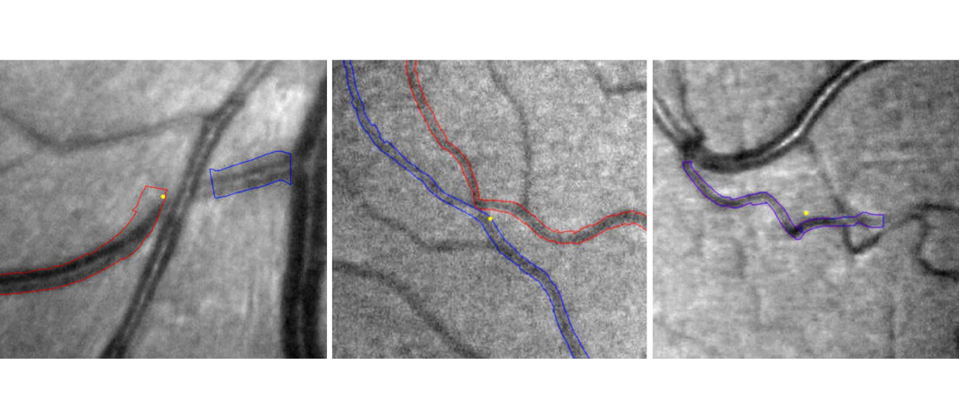
Refer to caption
(a)
Figure 15: Three problematical cases in the ETOS tracking algorithm[10]. From left to right: blurry crossing parts, small vessels with noise and small vessels with high curvature.

We aim to solve these problems via left-invariant contour enhancement processes on invertible orientation scores as pre-processing for subsequent tracking[10], recall Figure 2. In our enhancements, we rely on non-linear extension [33] of finite difference implementations of the contour enhancement process to improve adaptation of our model to the data in the orientation score. Finally, the ETOS tracking algorithm [10] is performed on the enhanced retinal images with respect to various problematic tracking cases, in order to show the benefit of the left-invariant diffusion on S​E​(2)SE(2).

As a proof of concept, we show examples of tracking on left-invariantly diffused invertible orientation scores on cases where standard ETOS-tracking without left-invariant diffusion fails, see Figure 16.

Refer to caption
Figure 16: Vessel tracking on retinal images. From up to down: the original retinal images with erroneous ETOS tracking, the enhanced retinal images with accurate tracking after enhancement.

All the experiments in this section use the same parameters. All the retinal images are selected with the size 400×400400\times 400. Parameters used for tracking are the same as the parameters of the ETOS algorithm in [10]: Number of orientations NoN_{o} = 36, wavelets-periodicity = 2​�2\pi. The following parameters are used for the non-linear coherence-enhancing diffusion (CED-OS): spatial scale of the Gaussian kernel for isotropic diffusion is ts=12​�s2=12t_{s}=\frac{1}{2}\sigma_{s}^{2}=12, the scale for computing Gaussian derivatives is ts′=0.15t_{s}^{\prime}=0.15, the metric �=0.058\beta=0.058, the end time t=20t=20, and c=1.2c=1.2 for controlling the balance between isotropic diffusion and anisotropic diffusion, for details see [33].

8 Conclusion

We analyzed linear left-invariant diffusion, convection-diffusion and their resolvents on invertible orientation scores, following both 3 numerical and 3 exact approaches. In particular, we considered the Fokker-Planck equations of Brownian motion for contour enhancement, and the direction process for contour completion. We have provided 3 exact solution formulas for the generic left-invariant PDE’s on S​E​(2)SE(2) to place previous exact formulas into context. These formulas involve either infinitely many periodic or non-periodic Mathieu functions, or only 4 non-periodic Mathieu functions.

Furthermore, as resolvent kernels suffer from severe singularities that we analyzed in this article, we propose a new time integration via Gamma distributions, corresponding to iterations of resolvent kernels. We derived new asymptotic formulas for the resulting kernels and show benefits towards applications, illustrated via stochastic completion fields in Figure 5.

Numerical techniques can be categorized into 3 approaches: finite difference, Fourier based and stochastic approaches. Regarding the finite difference schemes, rotation and translation covariance on reasonably sized grids requires B-spline interpolation [33] (towards a left-invariant grid), including additional numerical blurring. We applied this both to implicit schemes and explicit schemes with explicit stability bound. Regarding Fourier based techniques (which are equivalent to S​E​(2)SE(2) Fourier methods, recall Remark 4.3), we have set an explicit connection in Theorem 5.4 to the exact representations in periodic Mathieu functions from which convergence rates are directly deduced. This is confirmed in the experiments, as they perform best in the numerical comparisons.

We compared the exact analytic solution kernels to the numerically computed kernels for all schemes. We computed the relative ℓ1\ell_{1} and ℓ2\ell_{2} errors in both spatial and Fourier domain. We also analyzed errors due to Riemann sum approximations that arise by using the DFT−1\textbf{DFT}^{-1} instead of using the CFT−1\textbf{CFT}^{-1}. Here, we needed to introduce a spatial Gaussian blurring with small “inner-scale” due to finite sampling. This small Gaussian blurring allows us, to control truncation errors, to maintain exact solutions, and to reduce the singularities. We implemented all the numerical schemes in Mathematica, and constructed the exact kernels based on our own implementation of Mathieu functions to avoid the numerical errors and slow speed caused by Mathematica’s Mathieu functions.

We showed that FBT, stochastic and FD provide reliable numerical schemes. Based on the error analysis we demonstrated that best numerical results were obtained using the FBT with negligible differences. The stochastic approach (via a Monte Carlo simulation) performs second best. The errors from the FD method are larger, but still located in an admissible scope, and they do allow non-linear adaptation. Preliminary results in a retinal vessel tracking application show that the PDE’s in the orientation score domain preserve the crossing parts and help the ETOS algorithm[10] to achieve more robust tracking.

Acknowledgements

The research leading to the results of this article has received funding from the European Research Council under the European Community’s 7th Framework Programme (FP7/2007-2014)/ERC grant agreement No. 335555. The China Scholarship Council (CSC) is gratefully acknowledged for the financial support No. 201206300010.

[Uncaptioned image]

Appendix A Invertible Orientation Scores of 2D-images and Continuous Wavelet Theory

The continuous wavelet transform constructed by unitary irreducible representations of locally compact groups was first formulated by Grossman et al. [36]. Given a Hilbert space HH and a unitary irreducible representation g↦𝒰}g\mapsto\mathcall{U}_{g} of any locally compact group GG in HH, a vector 0≠ ∈H0\neq\psi\in H is called admissible if

C:=∫G|(𝒰} , )|∈( , )H​d​�G​(g)<∞,\displaystyle C:=\int_{G}\frac{|(\mathcall{U}_{g}\psi,\psi)|^{2}}{(\psi,\psi)_{H}}d\mu_{G}(g)<\infty, (73)

where �G\mu_{G} denotes the left-invariant Haar measure. Given an admissible vector \psi and a unitary representation of a locally compact group GG in HH, the CS transform 𝒲~:H→L2​(G)\widetilde{\mathcall{W}}:H\rightarrow\mdmathbb{L}_{2}(G) is given by (𝒲~[f])(g)=(𝒰} ,{)ℋ(\widetilde{\mathcall{W}}[f])(g)=(\mathcall{U}_{g}\psi,f)_{H}. It is well known in mathematical physics [3], that 𝒲~\widetilde{\mathcall{W}} is an isometric transform onto a closed reproducing kernel space CKG\mdmathbb{C}_{K}^{G} with K(g,g′)=1C(𝒰} ,𝒰}′ )ℋK(g,g^{\prime})=\frac{1}{C}(\mathcall{U}_{g}\psi,\mathcall{U}_{g^{\prime}}\psi)_{H} as an L2\mdmathbb{L}_{2}-subspace.

Now in our orientation score transform f↦𝒲{f\mapsto\mathcall{W}f, Eq. (1), we restrict to disk-limited images** * Such a restriction is convenient and reasonable for applications in view of the Nyquist frequency. Nevertheless, it is not strictly necessary for an L2\mdmathbb{L}_{2}-isometry, when one extends continuous wavelets to distributional wavelet transforms [10, Thm 1,App. B].:

f∈L2%(R2)={g∈L2(R2)|suppℱℛ∈}⊂ℬ0,%},f\in\mdmathbb{L}_{2}^{\varrho}(\mdmathbb{R}^{2})=\{g\in\mdmathbb{L}_{2}(\mdmathbb{R}^{2})\;|\;\textrm{supp}\mathcall{F}_{\mdmathbb{R}^{2}}g\subset B_{\textbf{0},\varrho}\},

With B0,%={!∈R2|‖!‖≤%}B_{\textbf{0},\varrho}=\{\mbox{\boldmath$\omega$}\in\mdmathbb{R}^{2}\;|\;\|\mbox{\boldmath$\omega$}\|\leq\varrho\}, with %>0\varrho>0 close to the Nyquist-frequency. We set the left-regular representation g↦𝒰}g\mapsto\mathcall{U}_{g} given by (𝒰}=(x,�){)(y)={(ℛ�−∞(y−x))(\mathcall{U}_{g=(\textbf{x},\theta)}f)(\textbf{y})=f(R_{\theta}^{-1}(\textbf{y}-\textbf{x})) as the unitary representation.

We distinguish between the isometric wavelet transform 𝒲~:L2%​(R2)→L2​(G)\widetilde{\mathcall{W}}:\mdmathbb{L}_{2}^{\varrho}(\mdmathbb{R}^{2})\rightarrow\mdmathbb{L}_{2}(G) and the unitary wavelet transform 𝒲%:ℒ∈​(ℛ∈)→𝒞𝒦𝒢\mathcall{W}^{\varrho}:\mdmathbb{L}_{2}(\mdmathbb{R}^{2})\rightarrow\mdmathbb{C}_{K}^{G}, as they have different adjoint transforms. We drop the formal requirement of 𝒰\mathcall{U} being square-integrable and \psi being admissible in the sense of (73), as it is not strictly needed/applicable for lots of cases. This includes our case of interest G=S​E​(2)G=SE(2) and its left-regular action on L2​(R2)\mdmathbb{L}_{2}(\mdmathbb{R}^{2}) where 𝒲{(})=(𝒰} ,{)ℒ∈​(ℛ∈)\mathcall{W}f(g)=(\mathcall{U}_{g}\psi,f)_{\mdmathbb{L}_{2}(\mdmathbb{R}^{2})} gives rise to an orientation score. We call ∈L2​(R2)∩L1​(R2)\psi\in\mdmathbb{L}_{2}(\mdmathbb{R}^{2})\cap\mdmathbb{L}_{1}(\mdmathbb{R}^{2}) an admissible vector if

0<M⁡(!):=(2​�)​∫−��|ℱℛ∈​ ​(ℛ�−∞​!)|2​𝑑�<∞​ for all ​!∈B0,%.\displaystyle 0<M(\omega):=(2\pi)\int\limits_{-\pi}^{\pi}\left|\mathcall{F}_{\mdmathbb{R}^{2}}\psi(R^{-1}_{\theta}\omega)\right|^{2}\,{\rm d}\theta<\infty\text{ for all }\omega\in B_{\textbf{0},\varrho}. (74)

Note that L1​(R2)\mdmathbb{L}_{1}(\mdmathbb{R}^{2}) implies that ℱℛ∈​ \mathcall{F}_{\mdmathbb{R}^{2}}\psi and MM are continuous functions vanishing at infinity.

From the general theory of reproducing kernels spaces, see e.g. [3], [21, Thm.18,Cor.4], it follows that 𝒲:ℒ∈%​(ℛ∈)↦𝒞𝒦𝒮ℰ⁡(∈)\mathcall{W}:\mdmathbb{L}_{2}^{\varrho}(\mdmathbb{R}^{2})\mapsto\mdmathbb{C}_{K}^{SE(2)} is unitary, where CKS​E​(2)\mdmathbb{C}_{K}^{SE(2)} denotes the unique [4] reproducing kernel space consisting of complex-valued functions on S​E​(2)SE(2) with reproducing kernel

K(x,�)​(x′,�′)=(𝒰(x,�)​ ,𝒰(x′,�′)​ )ℒ∈​(ℛ∈).K_{(\textbf{x},\theta)}(\textbf{x}^{\prime},\theta^{\prime})=(\mathcall{U}_{(\textbf{x},\theta)}\psi,\mathcall{U}_{(\textbf{x}^{\prime},\theta^{\prime})}\psi)_{\mdmathbb{L}_{2}(\mdmathbb{R}^{2})}.

Unfortunately, the characterization of the inner-product and norm on the space of orientation scores CKS​E​(2)\mdmathbb{C}_{K}^{SE(2)} via its reproducing kernel is relatively complicated [42]. Therefore, we provide a basic characterization of this inner-product next. For an admissible vector ∈L2​(R2)\psi\in\mdmathbb{L}_{2}(\mdmathbb{R}^{2}), the span of {𝒰} |}∈𝒢}\{\mathcall{U}_{g}\psi\,|\,g\in G\}, is dense in L2​(R2)\mdmathbb{L}_{2}(\mdmathbb{R}^{2}). The next construction is in line with general admissibility conditions in [34, Ch.5].

Theorem A.1.

Let \psi be an admissible vector in the sense that (74) is satisfied. Then 𝒲:ℒ∈�​(ℛ∈)→𝒞𝒦𝒮ℰ⁡(∈)\mathcall{W}:\mdmathbb{L}_{2}^{\rho}(\mdmathbb{R}^{2})\to\mdmathbb{C}_{K}^{SE(2)} is unitary, and we have

(f,g)L2​(R2)=(𝒲{,𝒲})ℳ,(f,g)_{\mdmathbb{L}_{2}(\mdmathbb{R}^{2})}=(\mathcall{W}f,\mathcall{W}g)_{M},

where (U,V)M=(𝒯ℳ​𝒰,𝒯ℳ​𝒱)ℒ∈​(𝒮ℰ​(∈))(U,V)_{M}=(\mathcall{T}_{M}U,\mathcall{T}_{M}V)_{\mdmathbb{L}_{2}(SE(2))} with operator 𝒯ℳ:𝒞𝒦𝒮ℰ⁡(∈)→ℒ∈​(𝒮ℰ⁡(∈))\mathcall{T}_{M}:\mdmathbb{C}_{K}^{SE(2)}\to\mdmathbb{L}_{2}(SE(2)) given by

[𝒯ℳ𝒰](x,�)=ℱℛ∈−∞[!↦(∈�)−∞∈ℳ−∞∈(!)ℱℛ∈𝒰(!,�)](x).[\mathcall{T}_{M}U](\textbf{x},\theta)=\mathcall{F}_{\mdmathbb{R}^{2}}^{-1}\left[\omega\mapsto(2\pi)^{-\frac{1}{2}}M^{-\frac{1}{2}}(\omega)\mathcall{F}_{\mdmathbb{R}^{2}}U(\omega,\theta)\right](\textbf{x}).
Corollary A.2.

Let M⁡(!)>0M(\mbox{\boldmath$\omega$})>0 for all !∈R2\mbox{\boldmath$\omega$}\in\mdmathbb{R}^{2}. The space of orientation scores CKS​E​(2)\mdmathbb{C}_{K}^{SE(2)} is a closed subspace of H⊗L2​(S1)\mdmathbb{H}\otimes\mdmathbb{L}_{2}(S^{1}), where H:={f∈L2(R2)|M−12ℱℛ∈{∈ℒ∈(ℬ0,%)}\mdmathbb{H}:=\{f\in\mdmathbb{L}_{2}(\mdmathbb{R}^{2})\;|\;M^{-\frac{1}{2}}\mathcall{F}_{\mdmathbb{R}^{2}}f\in\mdmathbb{L}_{2}(B_{\textbf{0},\varrho})\}. The orthogonal projection P\mdmathbb{P} of H⊗L2​(S1)\mdmathbb{H}\otimes\mdmathbb{L}_{2}(S^{1}) onto CKS​E​(2)\mdmathbb{C}_{K}^{SE(2)} is given by

(PU)(x,�)=(K(x,�),U)M=(𝒲𝒲∗,⌉§⊔𝒰)(x,�),(\mdmathbb{P}U)(\textbf{x},\theta)=(K_{(\textbf{x},\theta)},U)_{M}=(\mathcall{W}\mathcall{W}^{*,ext}U)(\textbf{x},\theta),

where 𝒲∗,⌉§⊔:ℋ%⊗ℒ∈(𝒮∞)→ℒ∈(ℛ∈)\mathcall{W}^{*,ext}:\mdmathbb{H}^{\varrho}\otimes\mdmathbb{L}_{2}(S^{1})\to\mdmathbb{L}_{2}(\mdmathbb{R}^{2}) is the natural extension of the adjoint given by

𝒲∗,⌉§⊔𝒰=ℱℛ∈−∞[ℳ−∞ℱℛ∈[x↦∫−��(∗�+�𝒰(⋅,�))(x)⌈�]].\mathcall{W}^{*,ext}U=\mathcall{F}_{\mdmathbb{R}^{2}}^{-1}\left[M^{-1}\mathcall{F}_{\mdmathbb{R}^{2}}\left[\textbf{x}\mapsto\int\limits_{-\pi}^{\pi}({}_{\theta+\pi}*U(\cdot,\theta))(\textbf{x}){\rm d}\theta\right]\right]. (75)
Remark A.3.

In Theorem A.1 we have restricted ourselves to disk-limited images. In Corollary A.2 we did not apply such a restriction, as it is not needed. Indeed, if U∈HU\in\mdmathbb{H} is such that ℱ𝒰⁡(⋅,�)\mathcall{F}U(\cdot,\theta) has support outside the disk with radius %\varrho for all �∈(−�,�]\theta\in(-\pi,\pi], then it is mapped to zero in (75), i.e. then 𝒲∗,⌉§⊔𝒰=′\mathcall{W}^{*,ext}U=0.
However, in order to ensure that the Sobolev type of space H\mdmathbb{H} is a true L2\mdmathbb{L}_{2}-space endowed with L2\mdmathbb{L}_{2}-norm a restriction to disk limited images f∈L2%​(R2)f\in\mdmathbb{L}_{2}^{\varrho}(\mdmathbb{R}^{2}) is necessary, as MM is a continuous function vanishing at infinity. In that case (using L2%​(R2)\mdmathbb{L}_{2}^{\varrho}(\mdmathbb{R}^{2}), 0<%<∞0<\varrho<\infty, as input space) we need to replace H\mdmathbb{H} by the space H%:={f∈L2%(R2)|M−1ℱ{∈ℒ∈(ℛ∈)}\mdmathbb{H}^{\varrho}:=\{f\in\mdmathbb{L}_{2}^{\varrho}(\mdmathbb{R}^{2})\;|\;M^{-1}\mathcall{F}f\in\mdmathbb{L}_{2}(\mdmathbb{R}^{2})\}. In case MM is uniformly bounded from below on B0%B_{\textbf{0}}^{\varrho}, the set H%\mdmathbb{H}^{\varrho} coincides with the set L2%​(R2)\mdmathbb{L}_{2}^{\varrho}(\mdmathbb{R}^{2}), although it is equipped with a different equivalent norm. In case M=1B0,%M=1_{B_{\textbf{0},\varrho}}, the norms coincide and then H%⊗L2​(S1)=L2​(S​E​(2))\mdmathbb{H}^{\varrho}\otimes\mdmathbb{L}_{2}(S^{1})=\mdmathbb{L}_{2}(SE(2)), and (75) reduces to

(𝒲∗,⌉§⊔𝒰)(x)=∫−��(∗�+�𝒰(⋅,�))(x)⌈�=∫𝒮ℰ⁡(∈)𝒰(})(𝒰} )(x)⌈�𝒢(}).(\mathcall{W}^{*,ext}U)(\textbf{x})=\int\limits_{-\pi}^{\pi}({}_{\theta+\pi}*U(\cdot,\theta))(\textbf{x}){\rm d}\theta=\int\limits_{SE(2)}U(g)\;(\mathcall{U}_{g}\psi)(\textbf{x})\,{\rm d}\mu_{G}(g).

Appendix B Asymptotical Behavior of the Kernels around the Origin in the Fourier Domain

Asymptotical analysis is done for the contour enhancement case in B.1, while asymptotical analysis is done for the contour completion case in B.2.

B.1 Contour Enhancement Asymptotic Formulas along !�\omega_{\xi} and !�\omega_{\eta}-axis

By freezing cos2⁡('−�)=1\cos^{2}(\varphi-\theta)=1 and dividing by D33D_{33} within the generator in the Fourier domain Eq. (5.1). The formula are given as follows:

((D11D33�2+�D33)−∂�2)R^�D11,D33(!,⋅)=�2​�​D33�0�,\left((\frac{D_{11}}{D_{33}}\rho^{2}+\frac{\alpha}{D_{33}})-\partial_{\theta}^{2}\right)\hat{R}_{\alpha}^{D_{11},D_{33}}(\mbox{\boldmath$\omega$},\cdot)=\frac{\alpha}{2\pi D_{33}}\delta_{0}^{\theta}, (76)

in which �=!�=cos⁡�​!x+sin⁡�​!y\rho=\omega_{\xi}=\cos\theta\omega_{x}+\sin\theta\omega_{y}, and !=(�​cos⁡',�​sin⁡')∈R2\mbox{\boldmath$\omega$}=(\rho\cos\varphi,\rho\sin\varphi)\in\mdmathbb{R}^{2}. This is solved by making continuous fit of solutions in null-space akin to Figure 11. Then we find

R^�D11,D33​(!,⋅)=�2​�​D33​W�​{e�​�, for ​�≤0,e−�​�, for ​�≥0,\hat{R}_{\alpha}^{D_{11},D_{33}}(\mbox{\boldmath$\omega$},\cdot)=\frac{\alpha}{2\pi D_{33}W_{\rho}}\left\{\begin{array}[]{l}e^{\sqrt{\lambda}\theta},\textrm{ for }\theta\leq 0,\\ e^{-\sqrt{\lambda}\theta},\textrm{ for }\theta\geq 0,\end{array}\right. (77)

where �=D11D33​�2+�D33\lambda=\frac{D_{11}}{D_{33}}\rho^{2}+\frac{\alpha}{D_{33}}, and W�=2​�W_{\rho}=2\sqrt{\lambda} denotes the Wronskian according to Eq. (41). Then, the approximation of the exact solution for contour enhancement is written as:

R^�D11,D33​(�​cos⁡�,�​sin⁡�,�)≈�4​�​D33​e−�2​D11D33+�D33​|�|�2​D11D33+�D33,\hat{R}_{\alpha}^{D_{11},D_{33}}(\rho\cos\theta,\rho\sin\theta,\theta)\approx\frac{\alpha}{4\pi D_{33}}\frac{e^{-\sqrt{\rho^{2}\frac{D_{11}}{D_{33}}+\frac{\alpha}{D_{33}}}|\theta|}}{\sqrt{\rho^{2}\frac{D_{11}}{D_{33}}+\frac{\alpha}{D_{33}}}}, (78)

in which D33D11\frac{D_{33}}{D_{11}} should be small. Then, we can find the fundamental solution by taking lim�↓0R^�D11,D33​(!,�)�\lim_{\alpha\downarrow 0}\frac{\hat{R}_{\alpha}^{D_{11},D_{33}}(\boldsymbol{\omega},\theta)}{\alpha}, which can be represented as:

S^D11,D33​(�​cos⁡�,�​sin⁡�,�)≈14​�​1�​D11​D33−|�|4​�​D33+O⁡(�2)\hat{S}^{D_{11},D_{33}}(\rho\cos\theta,\rho\sin\theta,\theta)\approx\frac{1}{4\pi}\frac{1}{\rho\sqrt{D_{11}D_{33}}}-\frac{|\theta|}{4\pi D_{33}}+O(\theta^{2}) (79)

Similarly, we can also get the resolvent equation along !�−\omega_{\eta}- axis for small �\rho. Here we cannot freeze cos⁡('−�)=0\cos(\varphi-\theta)=0 because the �\rho dependence will be lost, and we must rely on higher order expansion producing the following asymptotic formula:

R^�D11,D33​(�​cos⁡�,�​sin⁡�,�)≈�4​�​1�2​D11​D33+�​D33−14​�​(1−e−�D33​|�|�​D33),\hat{R}_{\alpha}^{D_{11},D_{33}}(\rho\cos\theta,\rho\sin\theta,\theta)\approx\frac{\alpha}{4\pi}\frac{1}{\sqrt{\rho^{2}D_{11}D_{33}+\alpha D_{33}}}-\frac{1}{4\pi}\left(\frac{1-e^{-\sqrt{\frac{\alpha}{D_{33}}}|\theta|}}{\sqrt{\alpha}\sqrt{D_{33}}}\right), (80)

and again for 0<�≪10<\rho\ll 1

S^D11,D33​(�​cos⁡�,�​sin⁡�,�)≈14​�​1�​D11​D33−|�|4​�​D33.\hat{S}^{D_{11},D_{33}}(\rho\cos\theta,\rho\sin\theta,\theta)\approx\frac{1}{4\pi}\frac{1}{\rho\sqrt{D_{11}D_{33}}}-\frac{|\theta|}{4\pi D_{33}}. (81)

Conclusion: From Eq. (78) and (81), we deduce that R^�D11,D33​(!,�)\hat{R}_{\alpha}^{D_{11},D_{33}}(\boldsymbol{\omega},\theta) does not have a pole at !=0\boldsymbol{\omega}=0 for �>0\alpha>0. S^D11,D33​(!,�)\hat{S}^{D_{11},D_{33}}(\boldsymbol{\omega},\theta) has a pole of order 1 at !=0\boldsymbol{\omega}=0.

B.2 Contour Completion Asymptotic Formulas along !�\omega_{\xi} and !�\omega_{\eta}-axis

We again freeze cos⁡('−�)=1\cos(\varphi-\theta)=1 for '=�\varphi=\theta, i.e. along the !�\omega_{\xi}-axis, where �=!�=cos⁡�​!x+sin⁡�​!y\rho=\omega_{\xi}=\cos\theta\omega_{x}+\sin\theta\omega_{y} in the generator in the Fourier domain Eq. (5.1) and apply Taylor approximation. Then we have the approximation of the resolvent equation in the Fourier domain, which is given by

R^�D33​(�​cos⁡�,�​sin⁡�,�)≈�4​�​e−|�|​D33�+i​��​D33+i​�​D33\hat{R}_{\alpha}^{D_{33}}(\rho\cos\theta,\rho\sin\theta,\theta)\approx\frac{\alpha}{4\pi}\frac{e^{-\frac{|\theta|\sqrt{D_{33}}}{\sqrt{\alpha+i\rho}}}}{\sqrt{\alpha D_{33}+i\rho D_{33}}}\\ (82)

Note that the fundamental solution

S^D33​(�​cos⁡�,�​sin⁡�,�)\displaystyle\hat{S}^{D_{33}}(\rho\cos\theta,\rho\sin\theta,\theta) ≈lim�↓01�​R^�D33​(�​cos⁡�,�​sin⁡�,�)\displaystyle\approx\lim_{\alpha\downarrow 0}\frac{1}{\alpha}\hat{R}_{\alpha}^{D_{33}}(\rho\cos\theta,\rho\sin\theta,\theta) (83)
=14​�​�​e−|�|​D332​�​(cos⁡(|�|​D332​�−�4)−i​sin⁡(|�|​D332​�−�4)).\displaystyle=\frac{1}{4\pi\sqrt{\rho}}e^{-\frac{|\theta|\sqrt{D_{33}}}{\sqrt{2}\rho}}\left(\cos\left(\frac{|\theta|\sqrt{D_{33}}}{\sqrt{2}\rho}-\frac{\pi}{4}\right)-i\sin\left(\frac{|\theta|\sqrt{D_{33}}}{\sqrt{2}\rho}-\frac{\pi}{4}\right)\right).

Therefore, we do not have a pole in the resolvent kernel, but in the fundamental solution we have a pole of order 12\frac{1}{2} in the Fourier domain. The behavior at ∞\infty is given by

S^D33​(�​cos⁡�,�​sin⁡�,�)≈e−|�|​D332​�4​�​�.\hat{S}^{D_{33}}(\rho\cos\theta,\rho\sin\theta,\theta)\approx\frac{e^{-\frac{|\theta|\sqrt{D_{33}}}{\sqrt{2}\rho}}}{4\pi\sqrt{\rho}}. (84)

Unlike the enhancement case, we cannot expect local isotropy at the origin.

Appendix C Algorithm for Evaluation of Non-periodic Mathieu functions

Consider the Mathieu equation

y′′​(z)+(a−2​q​cos⁡(2​z))​y​(z)=0y^{\prime\prime}(z)+(a-2q\cos(2z))y(z)=0 (85)

for a≤0a\leq 0 and q≠0q\neq 0. The Floquet theorem [44] yields the existence of solutions

y⁡(z)=ei​�​(a,q)​z​∑�−∞∞e2​i​�​z​c2​�​(a,q)y(z)=e^{i\nu(a,q)z}\sum\limits_{\rho-\infty}^{\infty}e^{2i\rho z}c_{2\rho}(a,q) (86)

with �​(a,q)∈C\nu(a,q)\in\mdmathbb{C} the Floquet exponent (which is correctly implemented in Mathematica) and with (c2​�​(a,q))�∈Z∈ℓ2​(Z)(c_{2\rho}(a,q))_{\rho\in\mdmathbb{Z}}\in\ell_{2}(\mdmathbb{Z}). Now the ODE has real-valued coefficients and for our second type of exact formulas in Theorem 5.2 we are aiming for the two real-valued solutions

me�(z)→0 if z→∞,me−�(z)→0 if z→−∞,\begin{array}[]{l}\textrm{me}_{\nu}(z)\rightarrow 0\textrm{ if }z\rightarrow\infty,\ \ \textrm{me}_{-\nu}(z)\rightarrow 0\textrm{ if }z\rightarrow-\infty,\end{array}

with �¯=−�\overline{\nu}=-\nu and where we take the convention Im​(�)≥0\textrm{Im}(\nu)\geq 0. Substitution of (86) into the Mathieu ODE directly provides the two-fold recursion c2​�+2+−a+(2​�+�)2q​c2​�+c2​�−2=0, for all ​�∈Z,c_{2\rho+2}+\frac{-a+(2\rho+\nu)^{2}}{q}c_{2\rho}+c_{2\rho-2}=0,\textrm{ for all }\rho\in\mdmathbb{Z}, with c0c_{0} and c2c_{2} such that

lim�±∞|c2​�|1|�|=0,\lim\limits_{\rho\pm\infty}|c_{2\rho}|^{\frac{1}{|\rho|}}=0, (87)

cf. ​[44], from which it follows that (c2​�)�∈Z∈ℓ1​(Z)(c_{2\rho})_{\rho\in\mdmathbb{Z}}\in\ell_{1}(\mdmathbb{Z}) we deduce that the series representations are uniformly converging (Weierstrass criterium) and furthermore their limits are continuously differentiable. Now we have me−�​(z)=me�​(−z)\textrm{me}_{-\nu}(z)=\textrm{me}_{\nu}(-z) and the solutions are real-valued if c−2​�=c2​�¯c_{-2\rho}=\overline{c_{2\rho}}. The two-fold recursion is of the type

c2​�+2−D2​�​c2​�+c2​�−2=0,c_{2\rho+2}-D_{2\rho}c_{2\rho}+c_{2\rho-2}=0,

with D2​�=a−(2​�+�​(a,q))qD_{2\rho}=\frac{a-(2\rho+\nu(a,q))}{q} and we enter the theory of continued fractions via division by c2​�c_{2\rho}

f�=D2​�−1f�−1, with ​f�:=c2​�+2c2​�,f_{\rho}=D_{2\rho}-\frac{1}{f_{\rho-1}},\textrm{ with }f_{\rho}:=\frac{c_{2\rho+2}}{c_{2\rho}},

and indeed under condition (87)[44, Eq.(3), p.106] we obtain converging solutions of type II. For definitions see [44, Section 2.22, p.107].

Algorithm
input: a≤0a\leq 0, R∋q≠0\mdmathbb{R}\ni q\neq 0, L∈NL\in\mdmathbb{N} recursion-depth at last coefficient, 2​N+1∈N2N+1\in\mdmathbb{N} number of coefficients.
initialization: c0=1c_{0}=1, f0=1f_{0}=1, fN+L=1D2​(N+L)f_{N+L}=\frac{1}{D_{2(N+L)}}.
For k=1,…,N+L−2k=1,\ldots,N+L-2 do fN+L−k:=1D2​(N+L−k+1)−fN+L−k+1.f_{N+L-k}:=\frac{1}{D_{2(N+L-k+1)}-f_{N+L-k+1}}.
Then build (c2,…,c2​N)(c_{2},\ldots,c_{2N}) by c2​l=fl−1​c2​l−2c_{2l}=f_{l-1}c_{2l-2}, for l=1,…,Nl=1,\ldots,N.
Then build (c¯2​N,…,c¯2,1,c2,…,c2​N)(\overline{c}_{2N},\ldots,\overline{c}_{2},1,c_{2},\ldots,c_{2N}).
Then compute by means of DFT, me�​(z)\textrm{me}_{\nu}(z) and me−�​(z)\textrm{me}_{-\nu}(z) from their coefficients via Eq. ​(86).

Refer to caption
Figure 17: From left to right: the final contour enhancement kernel based on the Mathematica Mathieu functions, the final contour enhancement kernel based on our own implementation of Mathieu functions. Both kernels use the same plot range and parameter settings: D={1,0,0.03}\textbf{D}=\{1,0,0.03\}, �=0.025\alpha=0.025, with sampling size No=48N_{o}=48 and Ns=128N_{s}=128.

Compared to the implementation of the contour enhancement kernel based on the Mathematica Mathieu functions, our own implementation of Mathieu functions is more robust and does not suffer from the numerical problems. They are much faster, see Table 6. Figure 17 shows us the final kernels obtained by using the Mathieu functions of Mathematica (left) and our own implementation (right). The Mathematica Mathieu functions are shown to break down when the sampling enters into certain regions, especially with small angular diffusion. Another big advantage of our implementation is that the speed of sampling a kernel is almost 30 times faster than the Mathematica implementation. Table 6 shows us the time requirements of the two routines for different parameter settings. We can see that our own Mathieu based implementation (OMI) is even 30 times faster than the Mathematica Mathieu based implementation (MMI).

Table 5: Speed of two implementations (kernel size: 48×128×128)(\text{kernel size:}\,48\times 128\times 128)
Parameters MMI time (s) OMI time (s)
D={1,0,0.03},�=0.025\textbf{D}=\{1,0,0.03\},\;\alpha=0.025 4037 139
D={1,0,0.12},�=0.025\textbf{D}=\{1,0,0.12\},\;\alpha=0.025 3272 137
D={1,0,0.03},�=0.05\textbf{D}=\{1,0,0.03\},\;\alpha=0.05 3220 137
Table 6: *

Measurement method abbreviations: (OMI) - Own Mathieu based implementation, (MMI) - Mathematica Mathieu based implementation.

References

  • [1] M. Abramowitz and I. A. Stegun. Handbook of Mathematical Functions with Formulas, Graphs, and Mathematical Tables. Dover Publications, 1965.
  • [2] A. Agrachev, U. Boscain, J. P. Gauthier, and F. Rossi. The intrinsic hypoelliptic Laplacian and its heat kernel on unimodular Lie groups. Journal of Functional Analysis, 256:2621–2655, 2009.
  • [3] S.T. Ali, J.P. Antoine, and J.P. Gazeau. Coherent states, wavelets and their generalizations. Springer Verlag, New York, Berlin, Heidelberg, 1999.
  • [4] N. Aronszajn. Theory of reproducing kernels. Trans. Amer. Math. Soc, 68:337–404, 1950.
  • [5] T. Aubin. A course in differential geometry. Graduate studies in mathematics. American Mathematical Society, 2001.
  • [6] J. August. The curve indicator random field. PhD thesis, Yale University, 2001.
  • [7] J. August and S.W. Zucker. The curve indicator random field and Markov processes. IEEE-PAMI, Pattern Recognition and Machine Intelligence, 25(4), 2003.
  • [8] D. Barbieri, G. Citti, G. Cocci, and A. Sarti. A cortical-inspired geometry for contour perception and motion integration. Journal of Mathematical Imaging and Vision, 2014. Accepted and published digitally online.
  • [9] D. Barbieri, G. Citti, G. Sanguinetti, and A. Sarti. An uncertainty principle underlying the functional archtecture of V1. Journal Physiology Paris, 106:183–193, 2012.
  • [10] E.J. Bekkers, R. Duits, T. Berendschot, and B. ter Haar Romeny. A multi-orientation analysis approach to retinal vessel tracking. Journal of Mathematical Imaging and Vision, pages 1–28, 2014.
  • [11] G. Ben-Yosef and O. Ben-Shahar. A tangent bundle theory for visual curve completion. IEEE-PAMI, Pattern Recognition and Machine Intelligence, 34(7):1263–1280, 2012.
  • [12] U. Boscain, R. Chertovskih, J.P. Gauthier, and A. Remizov. Hypoelliptic diffusion and human vision: A semi-discrete new twist on the Petitot theory. SIAM Journal of Imaging, 2014.
  • [13] U. Boscain, R. Duits, F. Rossi, and Y. Sachkov. Curve cuspless reconstruction via sub-Riemannian geometry. SIAM Journal of Imaging. Accepted on ESAIM: Control, Optimization and Calculus of Variations (COCV), 2013.
  • [14] U. Boscain, J. Duplaix, J.P. Gautier, and F. Rossi. Anthropomorphic image reconstruction via hypoelliptic diffusion. SIAM J. Control Optim, 50:1309–1336, 2012.
  • [15] W. H. Bosking, Y. Zhang, B. Schofield, and D. Fitzpatrick. Orientation selectivity and the arrangement of horizontal connections in tree shrew striate cortex. The Journal of Neuroscience, 17(6):2112–2127, March 1997.
  • [16] R.J. Casson, G. Chidlow, Wood J.P., J.G. Crowston, and Goldberg I. Definition of glaucoma: clinical and experimental concepts. Clinical and Experimental Ophthalmology, 40(4):341–349, 2012.
  • [17] G. S. Chirikjian. Stochastic models, information theory, and Lie groups, volume 1 of Applied and Nuemrical Harmonic Analysis, 2013.
  • [18] G.S. Chirikjian and A.B. Kyatkin. Engineering applications of noncommutative harmonic analysis: with emphasis on rotation and motion groups. Boca Raton CRC Press, 2001.
  • [19] G. Citti and A. Sarti. A cortical based model of perceptional completion in the roto-translation space. Journal of Mathematical Imaging and Vision, 24(3):307–326, 2006.
  • [20] E.J. Creusen, R. Duits, A. Vilanova, and M.J. Florack. Numerical schemes for linear and nonlinear enhancement of DW-MRI. Numer. Math. Theor. Meth. Appl, 6(1):138–168, 2013.
  • [21] R. Duits. Perceptual organization in image analysis. PhD thesis, Eindhoven University of Technology, The Netherlands, Eindhoven. http://www.bmi2.bmt.tue.nl/Image-Analysis/People/RDuits/THESISRDUITS.pdf, September 2005.
  • [22] R. Duits, U. Boscain, F. Rossi, and Y. Sachkov. Association fields via cuspless sub-Riemannian geodesics in SE(2). Journal of Mathematical Imaging and Vision, 2013. In Press.
  • [23] R. Duits and B. Burgeth. Scale spaces on Lie groups. In Murli Sgallari and Paragios, editors, 1st International Conference on Scale Space and Variational Methods in Computer Vision, Lecture Notes on Computer Science., pages 300 –312. Springer-Verlag, Jun. 2007.
  • [24] R. Duits, M. Felsberg, G. Granlund, and B. M. ter Haar Romeny. Image analysis and reconstruction using a wavelet transform constructed from a reducible representation of the Euclidean motion group. International Journal of Computer Vision, 79(1):79–102, 2007.
  • [25] R. Duits and E.M. Franken. Left-invariant parabolic evolutions on SE​(2)\mbox{SE}(2) and contour enhancement via invertible orientation scores, part I: Linear left-invariant diffusion equations on SE​(2)\mbox{SE}(2). Quarterly of Appl. Math., A.M.S., 68:255–292, 2010.
  • [26] R. Duits and E.M. Franken. Left-invariant parabolic evolutions on SE​(2)\mbox{SE}(2) and contour enhancement via invertible orientation scores, part II: Nonlinear left-invariant diffusion equations on invertible orientation scores. Quarterly of Appl. Mathematics, A.M.S., 68:292–331, 2010.
  • [27] R. Duits and M. van Almsick. The explicit solutions of linear left-invariant second order stochastic evolution equations on the 2D-Euclidean motion group. Technical Report CASA-report, nr.43., Eindhoven University of Technology Dep. of mathematics and computer science. http://www.win.tue.nl/analysis/reports/rana05-43.pdf, 2005.
  • [28] R. Duits and E.M. Franken. Left-invariant stochastic evolution equations on SE(2) and its applications to contour enhancement and contour completion via invertible orientation scores. Eindhoven University of Technology, CASA report, see http://arxiv.org/abs/0711.0951 and http://www.win.tue.nl/casa/research/casareports/2007.html, 35:1–79,2007.
  • [29] R. Duits and M. van Almsick. The explicit solutions of linear left-invariant second order stochastic evolution equations on the 2D Euclidean motion group. Quart. Appl. Math., 66:27–67, 2008.
  • [30] N. Dungey, A.F.M. ter Elst, and D.W. Robinson. Analysis on Lie groups with polynomial growth. Birkhauser-Progress in Mathematics, 214, 2003.
  • [31] L.M.J. Florack, B.M. ter Haar Romeny, J.J. Koenderink, and A. Viergever. Scale and the differential structure of images. Image and Vision Computing, 10:376–388, 1992.
  • [32] E.M. Franken. Enhancement of crossing elongated structures in images. PhD thesis, Department of Biomedical Engineering, Eindhoven University of Technology, The Netherlands, Eindhoven. http://www.bmia.bmt.tue.nl/people/EFranken/PhDThesisErikFranken.pdf, October 2008.
  • [33] E.M. Franken and R. Duits. Crossing preserving coherence-enhancing diffusion on invertible orientation scores. International Journal of Computer Vision (IJCV), 85(3):253–278, 2009.
  • [34] H. Führ. Abstract Harmonic Analysis of Continuous Wavelet Transforms Springer Heidelberg-New York, 2005.
  • [35] B. Gaveau. Principe de moindre action, propagation de la chaleur et estimees sous elliptiques sur certains groupes nilpotents. Acta Mathematica, 139:96–153, 1977.
  • [36] A. Grossmann, J. Morlet, and T. Paul. Integral transforms associated to square integrable representations. J.Math.Phys., 26:2473–2479, 1985.
  • [37] L. Hörmander. Hypoellptic second order differential equations. Acta Mathematica, 119:147–171, 1968.
  • [38] D.H. Hubel and T.N. Wiesel. Receptive fields of single neurons in the cat’s striate cortex. The Journal of Physiology, 148:574–591, 1959.
  • [39] M.K. Ikram, Y.T. Ong, C.Y. Cheung, and T.Y. Wong. Retinal vascular caliber measurements: clinical significance, current knowledge and future perspectives. Ophthalmologica, 229(3):125–136, 2013.
  • [40] W.B. Jones and W.J. Thron. The method of fractional steps: the solution of problems of mathematical physics in several variables. Encyclopedia of Mathematics and its Applications (Book 11). Massachusetts: Addison-Wesley Publishing Company. ISBN 0-201-13510-8. 1980.
  • [41] S.N. Kalitzin, B.M. ter Haar Romeny, and M.A. Viergever. Invertible orientation bundles on 2D scalar images. In Scale-Space Theories in Computer Vision, pages 77–88. Springer, 1997.
  • [42] F.J.L. Martens. Spaces of analytic functions on inductive/projective limits of Hilbert Spaces PhD thesis, University of Technology Eindhoven, Department of Mathematics and Computing Science, Eindhoven, The Netherlands, 1988. http://alexandria.tue.nl/extra3/proefschrift/PRF6A/8810117.pdf
  • [43] A.P. Mashtakov, A.A. Ardentov, and Y.L. Sachkov. Parallel algorithm and software for image inpainting via sub-Riemannian minimizers on the group of rototranslations. Numerical Methods: Theory and Applications, 6(1):95–115, 2013.
  • [44] J. Meixner and F.W. Schaefke. Mathieusche funktionen und sphaeroidfunktionen. Springer, 1954.
  • [45] P. MomayyezSiakhal and K. Siddiqi. 3D stochastic completion fields for mapping connectivity in diffusion MRI. IEEE-PAMI, Pattern Recognition and Machine Intelligence, 35(4), 2013.
  • [46] D. Mumford. Elastica and computer vision. Algebraic Geometry and Its Applications. Springer-Verlag, pages 491–506, 1994.
  • [47] J. Petitot. Neurogéometrie de la vision–Modeles mathématiques et physiques des architectures fonctionelles. Les Éditions de l’École Polytechnique. 2008.
  • [48] H. Skibbe and M. Reisert. Left-invariant diffusion on the motion group in terms of the irreducible representations of SO(3). Preprint on arXiv:1202.5414v1, see http://arxiv.org/pdf/1202.5414v1.pdf. 2012.
  • [49] Y. Sachkov. Conjugate and cut time in the sub-Riemannian problem on the group of motions of a plane. ESAIM: COCV, 16(4):1018–1039, 2010.
  • [50] G.Sanguinetti. Invariant models of vision between phenomenology, image statistics and neurosciences. PhD thesis, Universidad de la Republica, Montevideo, Uruguay, 2011. https://www.colibri.udelar.edu.uy/bitstream/123456789/2902/1/San11.pdf
  • [51] A. Sarti and G. Citti. Neuromathematics of vision, volume 1 of Springer: Lecture Notes in Morphogenesis.
  • [52] U. Sharma and R. Duits. Left-invariant evolutions of wavelet transforms on the similitude group. Applied Computational Harmonic Analysis, 2014. Under Review.
  • [53] A.F.M. ter Elst and D.W. Robinson. Weighted subcoercive operators on Lie groups. Journal of Functional Analysis, 157:88–163, 1998.
  • [54] G.B. Thomas and R.L. Finney. Calculus and analytic geometry (9th ed.). Addison Wesley, 1996.
  • [55] M. Unser, A. Aldroubi, and M. Eden. B-spline signal processing: Part 1-theory. IEEE Transcations on Signal Processing, 41(2):821–832, 1993.
  • [56] M. van Almsick. Context models of lines and contours. PhD thesis, Eindhoven University of Technology, 2007.
  • [57] K. Yosida. Functional analysis. Springer, 1995.
  • [58] J. Zweck and L.R. Williams. Euclidean group invariant computation of stochastic completion fields using shiftable-twistable functions. Journal of Mathematical Imaging and Vision, 21(2):135–154, 2004.