Failure of topological rigidity results for the measure contraction property

Let us start with the easier example of Theorem 1.3 of a space $(X,{\sf d},\mathfrak{m})$ satisfying ${\sf MCP}(0,3)$ containing an isometric embedding of the euclidean real-line. As a subset of $\mathbb{R}^{2}$ the space $X$ is defined as

see Figure 1 for an illustration.

The distance ${\sf d}$ on the space is the $l^{\infty}$-distance (3.1). The measure $\mathfrak{m}$ restricted to the half-infinite line segment $L=(\mathbb{R}_{+}\times\{0\})$ is $\mathcal{H}^{1}\lower 3.0pt\hbox{$|_{L}$}$, where $\mathcal{H}^{1}$ is the one-dimensional Hausdorff measure. On the cone $C=\{(x,y)\in\mathbb{R}^{2}\,:\,x\leq-3|y|\leq 0\}$ we define $\mathfrak{m}$ as a weighted Lebesgue measure via

In other words, the projection of $\mathfrak{m}$ to the first coordinate is the Lebesgue measure $\mathcal{L}_{1}$ and the measure $\mathfrak{m}$ is equally distributed in $X\cap(\{x\}\times\mathbb{R})$ for all $x\in\mathbb{R}$.

Let us then check that the space $(X,{\sf d},\mathfrak{m})$ satisfies ${\sf MCP}(0,3)$. We will always transport measure linearly in the horizontal direction. Hence it is sufficient to check ${\sf MCP}(0,3)$ separately for sets $A_{\mathbf{x}}=\{(\mathbf{x},y)\in A\,:\,y\in\mathbb{R}\}$ with $\mathbf{x}\in\mathbb{R}$. There are several cases to check depending on the position of the measure $\mu_{0}=\delta_{(\tilde{x},\tilde{y})}$ and the coordinate $\mathbf{x}\in\mathbb{R}$.

If $\mathbf{x},\tilde{x}>0$, we are on the one-dimensional part and we have a unique geodesics from $(\tilde{x},\tilde{y})$ to $(\mathbf{x},y)$ and along such geodesics we have

If $\mathbf{x}<0<\tilde{x}$, we can transport using a set of geodesics such that each image of a geodesic is a subset of a set of the form

in other words, we first transport along a euclidean geodesic to the origin and then continue along $L$. See the first case in Figure 2. Then the induced optimal transport satisfies

Compared to the previous case the first equality has now change to an inequality due to the fact that the density might drop when we pass through the origin.

Next we have to check the different cases when $\tilde{x}<0$. Let us first look at the easier case where $\mathbf{x}<\tilde{x}$. In this case we can again use euclidean geodesics. Since the density of the reference measure $\mathfrak{m}$ with respect to $\mathcal{L}_{2}$ is increasing in $C$ as $x$ increases, we have the estimate

The final case is when $\tilde{x}<\mathbf{x}$. In this case we still have three subcases to select the geodesic(s) from $(\tilde{x},\tilde{y})$ to a point $(\mathbf{x},y)$. The division to subcases at $\frac{\tilde{x}}{2}$ is due to the fact that all geodesics from $(\tilde{x},\tilde{y})$ to $(\{\frac{\tilde{x}}{2}\}\times\mathbb{R})\cap C$ have the same length.

In the subcase $\tilde{x}<\mathbf{x}\leq\tilde{x}/2$ we simply take the euclidean geodesic. In the subcase $\tilde{x}/2<\mathbf{x}<0$ we take a geodesic that first goes along the euclidean geodesic from $(\tilde{x},\tilde{y})$ to $(\frac{\tilde{x}}{2},\frac{\tilde{x}y}{2\mathbf{x}})$ and then along the euclidean geodesic from $(\frac{\tilde{x}}{2},\frac{\tilde{x}y}{2\mathbf{x}})$ to $(\mathbf{x},y)$. See the second case in Figure 2. The third subcase is when $\mathbf{x}>0$. In this subcase we first spread the measure uniformly from $(\tilde{x},\tilde{y})$ to $\{\tilde{x}/2\}\times[-\tilde{x}/6,-\tilde{x}/6]$, then contract along the euclidean geodesics to the origin and then move to $(\mathbf{x},y)$ along the euclidean geodesic. See the third case in Figure 2. Now in the case $\tilde{x}<\mathbf{x}\leq\tilde{x}/2$ we have

In the case $\tilde{x}/2<\mathbf{x}$ we have

and

All cases now being checked we have shown that $(X,{\sf d},\mathfrak{m})$ satisfies ${\sf MCP}(0,3)$.

The space $(Y,{\sf d},\mathfrak{n})$ we describe here with the maximal diameter $\pi$ is similar to our previous example. As a subset of $\mathbb{R}^{2}$ the space $Y$ is defined as

where

See Figure 3 for an illustration. Again the distance ${\sf d}$ is the $l^{\infty}$-distance (3.1). The measure is similar to the measure $\mathfrak{m}$, but this time the projection of the measure to the interval $[-\pi/2,\pi/2]$ is of the form ${\mathrm{d}}\mathfrak{n}=\cos^{2}(x){\mathrm{d}}\mathcal{L}_{1}$. Again we define the measure in such a way that the density is constant on $(\{x\}\times\mathbb{R})\cap Y$ for all $x\in[-\pi/2,\pi/2]$. The projected space $({\mathtt{p}}_{1}Y,{\sf d}_{e},({\mathtt{p}}_{1})_{\sharp}\mathfrak{n})$ clearly satisfies ${\sf CD}(2,3)$. It is not that surprising that $(Y,{\sf d},\mathfrak{n})$ satisfies ${\sf MCP}(2,3)$: the projection deals with the long distances and on the other hand it is already known that sufficiently small balls in $\mathbb{R}^{n}$ with the $l^{\infty}$ norm satisfy ${\sf MCP}(n,n+1)$, see [29]. The transition from the one-dimensional part to the two-dimensional part can then be carried out similarly as in the previous example.

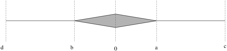
Nevertheless, let us check that the space $(Y,{\sf d},\mathfrak{n})$ really satisfies ${\sf MCP}(2,3)$. Let $A\subset Y$ with $\mathfrak{n}(A)>0$ and $(\tilde{x},\tilde{y})\in Y$. We again transport linearly in the horizontal direction and so it suffices to check that for all $\mathbf{x}\in[-\pi/2,\pi/2]$ we can select geodesics $\gamma$ from $(\tilde{x},\tilde{y})$ to $(\{\mathbf{x}\}\times\mathbb{R})\cap A$ such that

We again consider different cases separately depending on the position of $(\tilde{x},\tilde{y})$ and $\mathbf{x}$. First of all, if $1/4\leq|\mathbf{x}|,|\tilde{x}|\leq\pi/2$ we can take the measures $\mu_{t}$ to be uniformly distributed on the slices $(\{x\}\times\mathbb{R})\cap Y$. Since the space $({\mathtt{p}}_{1}Y,{\sf d}_{e},({\mathtt{p}}_{1})_{\sharp}\mathfrak{n})$ satisfies ${\sf CD}(2,3)$, we have the desired inequality (3.2) in this case.

The second case is when $|\mathbf{x}|\leq 1/4$ and $1/4\leq|\tilde{x}|\leq\pi/2$. In this case we take the geodesics along which we transport to be such that their images are subsets of sets of the type

Because inside $D$ we are changing the density as if we were transporting in $({\mathtt{p}}_{1}Y,{\sf d}_{e},({\mathtt{p}}_{1})_{\sharp}\mathfrak{n})$ and the density relative to this transport only drops when we leave $D$, again the fact that we have the inequality (3.2) follows from the observation that the space $({\mathtt{p}}_{1}Y,{\sf d}_{e},({\mathtt{p}}_{1})_{\sharp}\mathfrak{n})$ satisfies ${\sf CD}(2,3)$.

The final case to check is when $|\tilde{x}|\leq 1/4$. By symmetry we may assume that $\tilde{x}\leq\mathbf{x}$. As in the previous example we define the chosen geodesics from $(\tilde{x},\tilde{y})$ to a point $(\mathbf{x},y)\in A$ in three subcases. This time the division to subcases is driven by the fact that the distances from $(\tilde{x},\tilde{y})$ to all the points in $(\{(1/4+4\tilde{x})/5\}\times\mathbb{R})\cap D$ are equal, meaning that beyond that distance we can transport along vertically uniformly distributed measures.

Let us list the subcases. First, if $\tilde{x}<\mathbf{x}\leq(1/4+4\tilde{x})/5$, we take the euclidean geodesics. In the subcase $(1/4+4\tilde{x})/5<\mathbf{x}<1/4$ we take a geodesic that first goes along the euclidean geodesic that goes via the point $(1/4,0)$ from $(\mathbf{x},y)$ to $(\max\{0,(1/4+4\tilde{x})/5\},y^{\prime})$ and then along the euclidean geodesic from $(\max\{0,(1/4+4\tilde{x})/5\},y^{\prime})$ to $(\tilde{x},\tilde{y})$. The third subcase is when $\mathbf{x}>1/4$. In this subcase we first transport the mass along the euclidean geodesic to the point $(1/4,0)$, then spread the measure uniformly to $(\{\max\{0,(1/4+4\tilde{x})/5\}\}\times\mathbb{R})\cap D$ along euclidean geodesics and finally contract it to $(\tilde{x},\tilde{y})$ along euclidean geodesics.

Let us check the density in the different subcases. To deal with the first subcase $\tilde{x}<\mathbf{x}\leq(1/4+4\tilde{x})/5$ we observe that $h_{t}\leq(5/4-t/4)h_{1}$ for the vertical height $h_{t}$ of $D$ at $\gamma_{t}$, where $\gamma$ is a geodesic from $(\tilde{x},\tilde{y})$ to $(\mathbf{x},y)$. From this (and the estimates below) we have that

for all $t\in(0,1]$ and $l\in(0,1/2]$ and so (3.2) follows. (To see the third inequality in (3.3) define $f_{l}(t):=\left(\frac{5}{4}-\frac{t}{4}\right)\sin^{2}(tl)-t\sin^{2}(l)$ and notice that $f_{l}(t)\leq 0$ for all $t\in[0,1]$ and $l\in(0,1/2]$ since $f_{l}(0)=f_{l}(1)=0$ and $f_{l}^{\prime\prime}(t)=-\frac{l}{2}\sin(2tl)+(5-t)\frac{l^{2}}{2}\cos(2tl)\geq 0$ for all $t\in[0,1]$ and $l\in(0,1/2]$.)

In the second and third subcases $(1/4+4\tilde{x})/5<\mathbf{x}$, until we hit $(\max\{0,(1/4+4\tilde{x})/5\},y^{\prime})$ we have (3.2) by the projection as before. After $(\max\{0,(1/4+4\tilde{x})/5\},y^{\prime})$ we have (3.2) by the estimate (3.3) for $l\in(0,\frac{1}{2}]$. When $l>\frac{1}{2}$ we can estimate the time $t_{0}$ when we hit $(\max\{0,(1/4+4\tilde{x})/5\},y^{\prime})$ by

In this case obtaining (3.2) is easy, since verifying (3.3) for $t\in[0,\frac{1}{5}]$ and $l\in(\frac{1}{2},\frac{\pi}{2}+\frac{1}{4})$ reduces to verifying that $f_{l}(t)\leq 0$ for such $t$ and $l$. This follows for example by estimating

for $t\in[0,\frac{1}{5}]$ and $l\in(\frac{1}{2},\frac{\pi}{2}+\frac{1}{4})$. This completes the proof of the ${\sf MCP}(2,3)$ condition for our space $(Y,{\sf d},\mathfrak{n})$.

Both of our examples above had boundary points in the sense that there are geodesics that cannot be infinitely extended as local geodesics. It is natural to ask if one can modify the examples to have no boundary. By identifying the top and bottom boundaries in the two-dimensional parts of the spaces we should be able to get rid of most of the boundary points. However, even after the identification the point where the space changes from one-dimensional to two-dimensional will be a boundary point in the above sense. The nonextendable geodesics are the nonvertical geodesics in the two-dimensional side that are travelling more in the vertical direction than in the horizontal direction. When they reach the point where the dimension changes they cannot be extended to the one-dimensional part so that they are geodesic in a neighbourhood of the point where the dimension changes.

It is also interesting to consider the tangent spaces of the spaces $(X,{\sf d},\mathfrak{m})$ and $(Y,{\sf d},\mathfrak{n})$ in the sense of measured Gromov-Hausdorff limits of blow-ups. First observation is that the space $(X,{\sf d},\mathfrak{m})$ is the mGH-tangent of $(Y,{\sf d},\mathfrak{n})$ at the points $(a,0)$ and $(-a,0)$. This way we could prove the fact that $(X,{\sf d},\mathfrak{m})$ satisfies ${\sf MCP}(0,3)$ by proving that any tangent of a ${\sf MCP}(K,3)$ space does.

Notice that the tangents of $(X,{\sf d},\mathfrak{m})$ at points $X\setminus\{(0,0)\}$ and $(Y,{\sf d},\mathfrak{n})$ at points $Y\setminus\{(1/4,0),(-1/4,0)\}$ are all convex subsets of normed spaces. On the other hand we know from [14] that some subRiemannian spaces like the Heisenberg group satisfy ${\sf MCP}(K,N)$. With only such nice examples at hand it is natural to ask what are the tangent spaces of ${\sf MCP}(K,N)$ spaces (almost everywhere) in general? This is also related to the uniqueness of the tangents, compare to the following result by Le Donne [17].

References

- [1] L. Ambrosio, N. Gigli, A. Mondino and T. Rajala, Riemannian Ricci curvature lower bounds in metric measure spaces with -finite measure, arxiv:1207.4924, (2012), to appear on Trans. Amer. Math. Soc.
- [2] L. Ambrosio, N. Gigli and G. Savaré, Metric measure spaces with Riemannian Ricci curvature bounded from below, Preprint, arXiv:1109.0222, (2011), to appear on Duke Math. J.
- [3] L. Ambrosio, A. Mondino, and G. Savaré, Nonlinear diffusion equations and curvature conditions in metric measure spaces, In progress, (2013).
- [4] L. Ambrosio, A. Mondino, and G. Savaré, On the Bakry-Émery condition, the gradient estimates and the Local-to-Global property of metric measure spaces Preprint, arXiv:1309.4664, (2013).
- [5] K. Bacher and K.-T. Sturm, Localization and tensorization properties of the curvature-dimension condition for metric measure spaces, J. Funct. Anal., 259 (2010), 28–56.
- [6] F. Cavalletti, Decomposition of geodesics in the Wasserstein space and the globalization property, arXiv:1209.5909, (2012), to appear on Geom. Funct. Anal.
- [7] F. Cavalletti and K.-T. Sturm, Local curvature-dimension condition implies measure-contraction property, J. Funct. Anal., 262 (2012), 5110–5127.
- [8] J. Cheeger and D. Gromoll, The splitting theorem for manifolds of nonnegative Ricci curvature, J. Differential Geometry, 6 (1971/72), 119–128.
- [9] Y. Cheng, Eigenvalue comparison theorems and its geometric applications, Math. Z. 143 (1975), 289–297.
- [10] M. Erbar, K. Kuwada and K.-T. Sturm, On the equivalence of the entropic curvature-dimension condition and Bochner’s inequality on metric measure spaces, Preprint, arXiv:1303.4382, (2013).
- [11] N. Gigli, The splitting theorem in non-smooth context, Preprint, arXiv:1302.5555, (2013).
- [12] N. Gigli, A. Mondino and T. Rajala, Euclidean spaces as weak tangents of infinitesimally Hilbertian metric spaces with Ricci curvature bounded below, arXiv:1304.5359, (2013), to appear in J. Reine Angew. Math.
- [13] N. Gigli, T. Rajala and K.-T. Sturm, Optimal maps and exponentiation on finite dimensional spaces with Ricci curvature bounded from below, Preprint, arXiv:1305.4849, (2013).
- [14] N. Juillet, Geometric inequalities and generalized Ricci bounds in the Heisenberg group, Int. Math. Res. Notices 2009 (2009), 2347–2373.
- [15] C. Ketterer, Cones over metric measure spaces and the maximal diameter theorem, Preprint, arXiv:1311.1307, (2013).
- [16] Y. Kitabeppu, Lower bound of coarse Ricci curvature on metric measure spaces and eigenvalues of Laplacian, to appear on Geom. Dedicata, doi:10.1007/s10711-013-9844-3
- [17] E. Le Donne, Metric spaces with unique tangents, Ann. Acad. Sci. Fenn. Math. 36 (2011), no. 2, 683–694.
- [18] J. Lott and C. Villani, Ricci curvature for metric-measure spaces via optimal transport, Ann. of Math. 169 (2009), no. 3, 903–991.
- [19] S.-i. Ohta, Examples of spaces with branching geodesics satisfying the curvature-dimension condition, to appear on Bull. Lond. Math. Soc.
- [20] S.-i. Ohta, On the measure contraction property of metric measure spaces, Comment. Math. Helv. 82 (2007), 805–828.
- [21] S.-i. Ohta, Products, cones, and suspensions of spaces with the measure contraction property, J. Lond. Math. Soc. (2) 76 (2007), 225–236.
- [22] S.-i. Ohta, Splitting theorems for Finsler manifolds of nonnegative Ricci curvature, to appear in J. Reine Angew. Math.
- [23] Y. Ollivier, Ricci curvature of Markov chains on metric spaces, J. Funct. Anal. 256 (2009), 810–864.
- [24] T. Rajala, Failure of the local-to-global property for spaces, arXiv:1305.6436, (2013), to appear in Ann. Sc. Norm. Super. Pisa Cl. Sci.
- [25] T. Rajala, Interpolated measures with bounded density in metric spaces satisfying the curvature-dimension conditions of Sturm, J. Funct. Anal., 263 (2012), no. 4, 896–924.
- [26] T. Rajala, Local Poincaré inequalities from stable curvature conditions on metric spaces, Calc. Var. Partial Differential Equations, 44 (2012), no. 3–4, 477–494.
- [27] T. Rajala and K.-T. Sturm, Non-branching geodesics and optimal maps in strong -spaces, arXiv:1207.6754, (2012), to appear in Calc. Var. Partial Differential Equations.
- [28] K.-T. Sturm, On the geometry of metric measure spaces. I, Acta Math. 196 (2006), no. 1, 65–131.
- [29] K.-T. Sturm, On the geometry of metric measure spaces. II, Acta Math. 196 (2006), no. 1, 133–177.