Field emission from metal surfaces in the Thomas-Fermi-von-Weizsäcker model
Abstract
We evaluate the electron emission current density from jellium metallic surfaces in the Thomas-Fermi-von-Weizsäcker approximation. We implement the weighted density approximation (WDA) for description of the exchange and correlation energy of interacting electrons. We find electron-emission exhibits crossover from quantum to classical over-barrier escape of electrons from the surface barrier. Well below a surface-specific threshold field strength , electron tunneling is mainly affected by the change of the metal workfunction, and is less sensitive to the detailed shape of the surface barrier. In particular, since the position of the image charge plane for electrons leaving the surface does not precisely coincide with the centroid of the induced screening charge at the surface in response to the applied electrostatic field, we find an effective increase in the metal workfunction by eV, which decreases the dark current.
I Introduction
Metallic surfaces subject to strong electric field emit electrons into vacuum due tunneling transitions [1]. Employing the ballistic motion of emitted electrons in vacuum, field emission has found important practical applications in development of vacuum microelectronic devices [2], at the same time electron emission is an unwanted phenomenon in high-voltage vacuum insulation where it is considered as precursor to breakdown [3, 4]. Besides its technological importance and experimental interest, there remain relatively few calculations of the electron emission current using first-principles methods for description of the field-dsitroted surface electronic structure [5, 6, 7]. For the field emission from high work function surfaces Ref.[6, 7], the calculated electron current density complies qualitatively the Fowler-Nordheim (FN) model [1], which obeys a simple dependence upon the applied electric field , i.e.
| (1) |
where is the substrate workfunction, designates the position of the Fermi level relative to the lower edge of the valence band, is the Planck constant and and are the charge and mass of an electron, respectively.
Common to such model calculations is the use of an effective one-electron potential energy appropriate for vacuum tunneling, which is obtained in the framework of density functional theory (DFT) using the local density approximation (LDA) for the exchange and correlation energy. A well known drawback of LDA is that it fails to describe classical long-range image charge interaction between electron outside the surface and the polarization charge density that builds up at the surface in response to the Coulomb field of the escaping electron. Image charge interactions are also known to affect measured conductance of tunneling barriers arising in gallium-arsenide structures [12] and play an important role in the correct interpretation of STM measurements [13].
Nordheim [8] extended the FN model by including the Coulomb interaction energy of an electron at a distance from the surface with its induced self-image charge, where is the vacuum permittivity constant. This was discussed further in [9] and elaborated by Murphy and Good [10], the result for the current density including the image potential is
| (2) |
where at are slowly varying functions of the Nordheim parameter , and are related to certain linear combination of elliptic functions. Thus classical image charge effects take the form of multiplicative correction to the Fowler-Nordheim exponent. Normally it is assumed that Eq.2 remains valid for more realistic electron-surface potentials, because the main effect of reduction of the surface barrier occurs at distances where the classical image potential provides reasonable approximation. Thus Eq.(2) is used in the interpretation and analysis of experimental electron-emission data in terms of Fowler-Nordheim plot of as a function of the inverse field strength . Field enhancement factor is extracted from the slope and an effective emitting area from the intercept of the FN plot. These parameters depend on the surface roughness, morphology and other specific geometrical features of the emitting surface. To investigate influence of the surface barrier shape, more refined analysis of the FN plot has been developed [11], where slope and intercept correction factors are introduced in order to obtain more reliable values of the emission area and the field enhancement factor.
However Eq.(2) does not describe correctly the electron-surface interaction at small distances , where the classical image potential energy diverges. Within DFT [14] for a semi-infinite jellium model describing metal surface, the one-electron potential energy saturates to the local density exchange and correlation potential energy [15] close to the surface. Since electron tunneling is sensitive to the change of this potential energy, the motivation for the present work is development of more elaborate model for the surface barrier for electrons, which allows to quantify exchange and correlation effects in field emission from simple metal surfaces. The problem is simplified when the time spent by electrons under the barrier is long compared to the time required for the surface screening charges to build up [16, 17], such that dynamical screening effects may be neglected and the use quasistatic approximation for image charge interactions can be justified.
This paper is organized as follows. In Sec. II we give details on our theoretical model for field emission from arbitrarily structured metallic surfaces in the framework of density functional theory (DFT) in the Thomas-Fermi-von-Weizsäcker (TFvW) approximation [18, 19]. We treat image-charge interactions within the weighted density approximation (WDA) [20, 21] for the exchange and correlation energy of interacting electrons. In this way we obtain improved description of the electronic potential energy, which is regular close to the surface and exhibits correct image-charge behavior inside vacuum. In Sec. III we apply our method to field emission from jellium metallic surfaces and discuss numerical results. Sec. IV contains our main conclusions. Unless otherwise stated, we use atomic units () further throughout this work.
II Theoretical model
In hydrodynamical approximation, the electron gas is treated as a classical fluid which is characterized at each point in space by number density and velocity distributions. Neglecting dissipative effects, the electron dynamics is governed by the Euler’s equation
| (3) |
supplemented by the continuity equation for the density
| (4) |
Here is the internal energy of a static charged fluid, which we approximate within DFT
| (5) |
The first term gives the potential energy of the valence electrons in the electric field of the substrate ionic cores superimposed on an external uniform electric field applied to the surface. The second and third term represent the quantum-mechanical kinetic energy of non-interacting electrons in the TFvW approximation with phenomenological density gradient parameter . The value is used throughout this work as it gives good quantitative results for the ground-state workfunction and surface energy [22]. The last two terms are the repulsive Coulombic interaction energy and the exchange-correlation energy of the electrons, respectively. The exchange-correlation energy
| (6) |
is the Coulomb interaction energy between an electron at the point with its surrounding charge deficiency hole near
| (7) |
The exchange-correlation hole is given in terms of coupling-constant averaged electron-pair distribution function
| (8) |
here is the distribution function for electrons interacting via modified pairwise Coulomb potential of strength , but with one-particle density held fixed at the physical density () due to interaction of electrons with compensating -dependent external one-body potential [23]. By definition satisfies the sum rule
| (9) |
In the weighted-density-approximation [20, 24], we keep the one-particle density pre-factor in Eq.(7) and replace the exact pair-correlation function with that of a homogeneous electron gas of an auxiliary density , i.e.
| (10) |
where is the relative distance between pair of electrons. The effective density is a weighted average of the true electron density over the local Fermi wavelength . For regions of slowly varying density, the pre-factor in Eq.(7) can be treated as constant and brought in front of the integral in Eq.(6), resulting in LDA. The weighted-density parameter is chosen such that to satisfy the sum rule in Eq.(9). A model for the pair correlation function of the homogeneous electron gas is given by the ansatz [21]
| (11) |
in terms of two density parameters and . The long-range tail of the correlation factor ensures image-like behavior of the potential energy of an electron at large distances from the surface. The density functional in Eq.(7) with the approximation of Eq.(10) is also exact in several limiting cases: i) for the homogeneous electron gas, ii) for one-electron systems, such as hydrogen, where it gives exact cancellation of the electrostatic Coulomb self-interaction energy and iii) for an atom, where it reproduces the correct asymptotic form of the exchange-correlation energy density far from the nucleus.
At each point , the parameters and are functions of the weighted density , their density dependence is fixed by the satisfaction of the particle conservation sum rule
| (12) |
and by the requirement that the exchange and correlation energy per electron in an uniform system of number density is
| (13) |
We approximate with the sum of the Dirac exchange and the Wigner-corrected correlation energy, where is the Wigner-Seitz radius. The pair-correlation function is shown in Fig. 1 for bulk Wigner-Seitz radii and . It represents the tendency of electrons to avoid one another at small distances as a consequence of the short-range part of the repulsive Coulomb interaction and due to the Pauli repulsion between electrons in parallel spin component. Because tends to unity in a power-law way, electrons become weakly correlated at distances . A known drawback of this approximation is that the correlation factor becomes negative for low density substrates with , however it remains positive in the region of metallic densities .
II.1 Field emission from jellium metallic surfaces
As an application, we investigate the steady-state solutions of the hydrodynamical equations corresponding to field emission from simple jellium metallic surfaces. Here we assume the velocity distribution is described by an irrotational fluid flow (). The potential energy term represents the interaction of electrons with externally applied electric field superimposed on the electric field of a neutralizing charge distribution of the substrate ionic cores
| (14) |
where is the number density of the ionic charge distribution, is a pseudopotential correction to the ionic background potential, which takes in an average way the difference between the total pseudopotential of a discrete ion-lattice and the potential due to the uniform positive background. The pseudopotential parameter is choosen to make the jellium mechanically stable [25, 26] and does not cleave spontaneously. Due to the translation invariance of the jellium electronic structure in the surface plane, the number density and velocity distributions are functions of the coordinate normal to the surface, and . In this case, Eq. (3)-(4) expresses the conservation of the current density and the total energy per electron
| (15) |
here are the first and second derivatives of the electron density, is the chemical potential and
| (16) |
is a one-electron potential energy which is a superposition of the electrostatic Hartree and effective exchange and correlation energies, respectively. The Hartree potential satisfies the Poisson’s equation
| (17) |
subject to the boundary condition at . In WDA, the effective exchange-correlation potential is given approximately by
| (18) |
here
| (19) |
is the exchange and correlation energy per electron, and the functions and are given in terms of the incomplete gamma function . Inside vacuum, reproduces the correct classical image potential. Introducing the density variable , the Bernoulli equation Eq.(15) can be recast into a self-consistent Milne equation [27]
| (20) |
in terms of an effective one-electron potential energy
| (21) |
including the Thomas-Fermi kinetic pressure term and the Coulomb-derived Hartree and exchange-correlation potential energies. For convenience we set the zero of energy to . The boundary condition for the charge density inside vacuum can be written as for some constant , which we further associate with the centroid of the induced charge at surface in response to the external electric field and is the workfunction. In the metal interior , the electric field is fully screened by the conduction electrons and the density approaches the bulk density , such that we impose two additional boundary conditions for . The last two conditions constitute a system of algebraic equations for the integration constants and , which were solved by the Newton-Raphson method. Eq.(20) was solved self-consistently using the Bulirsch-Stoer method [28]. We use and .
III Numerical result and discussion
III.1 Charge density distribution
In Fig. 2 (a), for V/nm and V/nm we show the WDA induced charge density relative to the equilibrium distribution for . For the lower electric field V/nm, the density distribution is extended over the surface region and acts to screen the applied electric field inside the metal, charge transfer into vacuum is unlikely. In response to the increased field strength V/nm, the screening charge at the surface is enhanced, but the density distribution does not remain localized and extends into vacuum due to tunneling transitions. The resultant space-charge layer partially screens out the external electric field inside vacuum and near the surface, as Fig. 2(c) shows. Since the space-charge effect can be neglected for weak electric fields V/nm, the induced charge density profile is well characterized by its center-of-mass
| (22) |
which determines the effective location of the surface and also serves as a reference plane for the classical image potential [29]. The normalized LDA and WDA screening charge densities are shown in Fig.2(b) for the lowest electric field V/nm considered in this work. Also indicated is the center of the induced charge, which is positioned at a distance in front of the jellium edge for WDA and at for LDA. However the WDA density is much more diffuse, since the sharp density variations at the surface (which are more pronounced in the LDA) are averaged out over the range of the repulsive short-ranged electronic interactions. Since the WDA density approaches much more slowly the uniform bulk density in the metal interior, the external electric field is less efficiently screened (cf. Fig.2(c)). In response to increase of the field strength, the effective position of the surface shifts toward vacuum as shown in Fig. 2(d). That is because conduction electrons spill out at larger distances inside vacuum due to enhanced penetration of the barrier, in good qualitative agreement with the outward shift of for negatively charged surfaces reported in Ref.[30]. At high V/nm, the effective location of the surface is difficult to determine due to the formation of negative space charge layer inside vacuum (cf. Fig. 2(a)).
Fig. 3(a) shows the effective one-electron potential energy for sodium metallic surface () subject to an external electric field V/nm. The various locations of an electron inside the bulk (1), under the barrier (2) and inside vacuum (3) are indicated. Fig. 3(b-d) give the coupling-constant averaged exchange-correlation hole corresponding to the different positions (1-3) in Fig. 3(a). In the metal interior, cf. Fig.3(b), the hole is centered on the electron and the LDA approximation is adequate. When an electron changes its position and crosses the surface by moving outward under the barrier as shown in Fig.3(c), the hole does not follow and separates by spreading laterally along the surface plane. The center of the hole does not remain localized in the surface region and moves toward the bulk, as a consequence of the weighted density approximation. The electron is detached from the hole far inside vacuum as Fig.3(d) shows. The Coulomb attraction between the separated electron and hole charges gives rise to the classical image force exerted on the electron at large distances from the surface. Thus the asymptotic potential energy becomes
| (23) |
where specifies the position of the WDA image charge plane [31]
| (24) |
This image plane does not depend on any detail of the surface density distribution, thus given by the WDA is artificially fixed by the model for the pair correlation function of the uniform electron gas. More importantly is slightly shifted inside the jellium and does not coincide with the centroid of the induced (negative) screening charge at the surface. Despite this limitation of WDA, it is known that the screening response of a jellium substrate subjected to external electric fields of distinguishable test charges is characterized by which is different from experienced by electrons. For Al(111) surfaces, the position of the image charge plane is closer to the jellium edge than that predicted from classical response to external electric fields [32]. The importance of field emission in testing the equality between the parameters and has also been pointed in [29]. In Tab. I, we give values for the charge centroid and the WDA image-plane compared to other results. Our slightly overestimates the analytic result of Ref.[31], but otherwise gives negative . In contrast, the centroid of the induced screening charge lies in front of the surface and shifts toward the jellium edge with increase of the bulk density. Such variation of exhibits an opposite trend to LDA result for ordinary jellium [34]. This difference stems from the inclusion of the discrete ion-lattice effects in the stabilized jellium model, which in turn modify the screening properties of the metal (cf. Ref. [33]).
| Ref.[31] | Ref.[33] | Ref.[34] | |||
|---|---|---|---|---|---|
| 2 | -0.08 | -0.29 | 0.7 | 0.97 | 1.57 |
| 3 | -0.22 | -0.42 | 1.2 | 1.05 | 1.35 |
| 4 | -0.34 | -0.54 | 1.3 | 1.19 | 1.25 |
III.2 One-electron potentials
Fig.4(a) shows the field-dependence of the one-electron potential energy derived from the density distributions in Fig. 2(a). For comparison, the field-free potentials () are also shown. The zero-field WDA potential energy interpolates smoothly between the bulk LDA energy for large negative and the static image potential energy for large distances to the surface, as shown by the dotted line in Fig.4(a). In contrast the LDA potential energy falls exponentially with the distance, since it does not represent the non-local effect of separation of an electron from its exchange-correlation hole after the electron has moved inside vacuum. In response to moderate external electric field V/nm, the induced negative charge density at the surface lowers the height of the surface barrier and the width of the under-barrier region at the Fermi level becomes comparable to , which increases the probability for vacuum tunneling. The increased field strength continues to lower the barrier height and reduce the width of the surface barrier. For V/nm the top of the barrier (the Schottky saddle) moves below the position of the Fermi level to enable classically-allowed over-barrier transition.
In Fig.4(b), we plot the LDA and WDA surface barriers for V/nm and . For comparison the FN barrier and the modified Murphy-Good barrier are also shown. Here a modified MG barrier is introduced to incorporate the difference between the first moments of the induced screening-charge and image-charge distributions
| (25) |
If we choose as an effective position of the surface, the potential energy in Eq.(25) becomes identical with the classical MG result but with upshifted workfunction , where is the separation between the centroid of the induced negative charge density and the image charge plane experienced by electrons leaving the surface. It is worth to note that the effect of the workfunction increase is the same as if the surface is covered with electronegative adsorbates, such that the contribution of the induced dipole layer increases the substrate workfunction. The effective potential energy of Eq.(25) reproduces well the WDA result up to very small distances as Fig.4(b) makes evident. In contrast, the LDA barrier exhibits only weakly reduced height and width due to neglect of image charge interaction, and thus follows more closely the triangular Fowler-Nordheim barrier. The change of the surface barrier height and width due to change of the external electric field is shown in Fig.4(c-d). In the modified MG model, the reduced barrier height for electrons near Fermi level is
| (26) |
As Fig.4(c) demonstrates, the modified MG barrier height is nearly indistinguishable from the WDA result up to V/nm. Above V/nm, the WDA barrier height reduces much more slowly due to build up of the vacuum space charge layer, where self-electric fields of mobile electrons oppose the external field, such that the total electric field is weakened at the surface. In contrast, the LDA barrier felt by electrons at Fermi level is much higher at low electric fields and decreases linearly with the increased field strength , i.e.
| (27) |
where fit to the LDA barrier height gives V/nm. The differences between the LDA and WDA barrier heights diminishes at high V/nm, when the Schottky saddle has moved below the position of the Fermi level and electron transfer becomes classically allowed. Below threshold , the LDA barrier breadth follows quantitatively the prediction of the Fowler-Nordheim model as shown in Fig.4(d). Similarly the WDA barrier breadth follows closely the modified MG result , where is the modified Nordheim parameter given in terms of the square-root field strength and the effective workfunction . At these relatively weak electric electric fields V/nm, the LDA barrier breadth is thicker than the WDA breadth by nearly bohr radii, such that electron tunneling is much more likely in WDA. Using these parameters, the barrier transmission coefficient can be approximated by , after assuming that the multiplicative pre-exponential factor of the tunneling rate changes negligibly with . For tunneling out of the LDA barrier we get
| (28) |
and hence the screening response of conduction electrons is expressed by a correction factor to the Fowler-Nordheim exponent. The slope of the LDA tunneling rate (below threshold) is given by
| (29) |
so that the LDA slope is steeper relative to the field-independent Fowler-Nordheim slope , when the LDA slope converges . Quite similarly, the WDA result
| (30) |
is given in in terms of slowly-varying barrier reduction factor , which in contrast to LDA is primary due to self-image charge screening. The corresponding slope with , since for , the WDA slope is flatter relative to . Thus for relatively weak fields, the slope of the WDA emission rate is also flatter than the LDA one. However for sufficiently weak fields V/nm, the effects of the barrier reduction factors are weakened, hence the slopes and should merge into the FN slope. But since the LDA workfunction is increased by eV relative to the WDA result (cf. Tab. II for ), the difference of the slopes depends only on the difference of the model workfunctions. In order to verify such a qualitative estimate, in Fig.5(a-b) we plot the WKB emission rate and its slope for an electron at the Fermi level,
| (31) |
where and are the inner and outer turning points of the potential, for comparison the ordinary and modified MG results are also shown. The ordinary MG result is obtained from Eq.(25) by setting , i.e. neglecting finite differences between classical and the WDA image-charge planes. As 5(a) demonstrates, the modified MG and WDA emission rates are indistinguishable up to V/nm, when the WDA emission becomes slower relative to the modified MG result due to the space charge effect. In contrast field emission in LDA is highly unlikely, as it suppressed by more than one order of magnitude relative to the WDA result. The ordinary MG emission rate is the highest and overestimates the WDA result by a factor of 5. To understand this enhancement, Taylor expansion of the exponent in Eq.(30) for sufficiently weak fields results in , where and is the ordinary MG emission rate. For , we have and , thus , thereby reducing the modified MG emission rate relative to the ordinary MG result by such a factor due to weak field-induced increment of the substrate work-function by eV.
III.3 Current densities
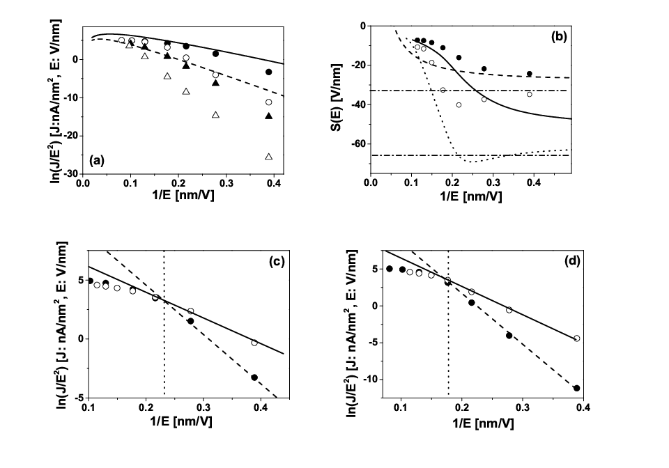
In Fig.6(a) we plot as a function of for aluminum () and sodium () surfaces. For weak fields, the overall trend of decrease of with the increase of the substrate work-function is clearly exhibited in the TFvW model. For the lower screening radius , the LDA and WDA-FN plots are approximately linear functions of , in good qualitative agreement with the modified MG result. A quantitative difference stems from the steeper slope of the WDA tunneling rate relative to the MG result. This difference is a direct consequence of the TFvW approximation for the kinetic energy, which gives density distributions that are less extended into vacuum, because the inverse decay length of the TFvW charge density is two times larger than the equilibrium inverse decay length . Similar conclusion can be drawn for the lower density jellium with . Noticeably, however the LDA rates exhibit even steeper slope relative to the WDA result: for V/nm and , the LDA current density , while the WDA result is larger by two orders of magnitude, as a consequence of the decreased WDA workfunction.
For the lower density jellium and electric field V/nm, the slope of our FN plot is flatter than that at lower . The non-linearity of the FN plot agrees with the result reported in Ref.[5], which was attributed to combination of several factors, such as finite energy width of the distribution of emitted electrons, finite probability for overbarrier reflection at the surface and the space charge effect. As our LDA and WDA results become indistinguishable at high , this effect is insensitive to the description of electron correlations. This non-linearity in the FN plot is due to build up of the space charge layer inside vacuum (cf. Fig.2(a,c)) that partially screens out the applied field inside vacuum, which tends to drive back electrons into the metal. This effect flattens out the slope of the FN plot and limits the increase of the current with the increased field strength, consistent with the classical Child-Langmuir law [36, 37].
To analyze this further, in Fig.6(b), we plot the slope of the FN plot as a function of the inverse field strength for . For comparison, the modified MG and FN slopes are also shown. At low V/nm, and are slowly varying functions of , but are steeper as compared to the MG and FN curves, because of the reduced density gradient in the TFvW approximation (as noted above). The LDA and WDA slopes converge to the shifted Fowler-Nordheim slope for low . The WDA slope flattens with the increase of and continuously crosses over to the Child-Langmuir behavior for V/nm. In contrast, the LDA slope steepens with the increase of , attains a minimum near V/nm and flattens out to merge with the WDA rate near V/nm. The WKB result for the electron-emission from the LDA and WDA surface barriers exhibits qualitatively similar trend. But due to the increased decay length of the electron density inside vacuum, the WKB slopes are shifted upward relative to the TFvW slopes at low , and converge to the Fowler-Nordheim slope . At higher V/nm, the WKB slopes are nearly indistinguishable from the TFvW ones. Thus the quantitative difference between TFvW and WKB rates is solely due to the reduced density gradient , which affects electron spill out inside vacuum.
Thus for relatively weak electric fields below some surface-specific threshold field strength , the TFvW result follows qualitatively the Fowler-Nordheim model in terms of the exponential formula
| (32) |
The density dependent parameters and were extracted from fit of the numerical result to Eq.(32) and given in Tab. II. The TFvW slope parameter coincides with the shifted Fowler-Nordheim slope , but the TFvW pre-factors exceed the MG and FN results by few orders of magnitude. For comparison, the corresponding WKB slope and pre-exponential factors are also given in Tab.II, the WKB slopes are flatter and tend to agree qualitatively with the ordinary Fowler-Nordheim result. Fig.6(c-d) shows comparison of the WKB and TFvW current densities for the LDA and WDA barriers. Above the threshold these current densities are almost indistinguishable, so the high-field part of the FN plot is unaffected by the approximation for noninteracting kinetic energy. The effect of the TFvW kinetic energy is to steepen the LDA and WDA slopes relative to the WKB result just below the threshold . As a consequence the WKB pre-exponential factors are reduced and move closer to the values predicted by the classical FN and modified MG results. In both cases, the lowered WDA workfunction relative to LDA is an essential factor in increasing the emission current.
| 2 | |||||
| TFvW-LDA | 4.01 | 19 | -100 | 5.3[-4] | |
| TFvW-WDA | 3.62 | 17 | -81 | 1.1[-2] | |
| FN | 4.01 | -55 | 6.3[-7] | ||
| MG | 3.62 | -44 | 6.5[-6] | ||
| WKB-LDA | 4.01 | 19 | -55 | 7.8[-4] | |
| WKB-WDA | 3.62 | 17 | -37 | 3.1[-4] | |
| 4 | |||||
| TFvW-LDA | 2.85 | 5.0 | -64 | 1.1[-3] | |
| TFvW-WDA | 2.65 | 4.5 | -48 | 3.4[-3] | |
| FN | 2.85 | -33 | 1.0[-6] | ||
| MG | 2.65 | -26 | 1.7[-4] | ||
| WKB-LDA | 2.85 | 5.0 | -37 | 2.1[-4] | |
| WKB-WDA | 2.65 | 4.5 | -23 | 5.2[-5] |
IV Conclusion
We have evaluated the field emission current from jellium metallic surfaces in the framework of quasi-static Thomas-Fermi-von-Weizsäcker model. Our result deviates from the Fowler-Nordheim model for strong electric fields due to space charge effects. In the tunneling regime we find the emission mechanism depends sensitively on the properties of the surface electronic structure and the approximations for kinetic and exchange-correlation energies, which in turn affect the substrate workfunction. As a consequence, we find that the conventional local-density-approximation underestimates the emission current by few orders of magnitude relative to the result of the weighted-density-approximation. We also find that the WDA emission current is decreased relative to the classical Murphy-Good result due to effective increase of the substrate workfunction by eV, which is due to the relative displacement between the WDA image charge plane experienced by electrons leaving the surface and the centroid of the induced screening charge density at the surface.
Acknowledgments
The authors acknowledge financial support by the ANR-12-BS09-0013-02 grant.
References
- [1] R. Fowler and L. Nordheim, Proc. R. Soc. Lond. A 119 (1928).
- [2] G. Fursey, Field emission in Vacuum Microelectronics Kluwer Academic/Plenum Publishers, New York (2005).
- [3] R. V. Latham, High voltage vacuum insulation: Basic concepts and technological practice, Academic Press, London (1995).
- [4] A. Simonin, H. de Esch, L. Doceul, L. Christin, F. Faisse, F. Villecroze, Fusion Engineering and Design 88, 1 (2013).
- [5] Y. Gohda, Y. Nakamura, K. Watanabe and S. Watanabe, Phys. Rev. Lett. 85, 1750 (2000).
- [6] T. Ohwaki, H. Ishida and A. Liebsch, Phys. Rev. B 68, 155422 (2003).
- [7] I. Merrick and J. E. Inglesfield , G. A. Attard, Phys. Rev. B 72, 033403 (2005).
- [8] L. W. Nordheim, Proc. Roy. Soc. Lond. A 121, 626 (1928).
- [9] R. F. Burgess, H. Kroemer and J. M. Houston, Phys. Rev. 90, 515 (1953).
- [10] E. L. Murphy and R. H. Good, Jr., Phys. Rev. 102, 1464 (1956).
- [11] R. G. Forbes, Nanotechnology 23, 095706 (2012).
- [12] P. Gueret, E. Marclay and H. Meier, Appl. Phys. Lett 53, 1617 (1988).
- [13] G. Binnig, N. Garcia, H. Rohrer, J. M. Soler, F. Flores, Phys. Rev. B 30, 4816 (1984).
- [14] N. D. Lang and W. Kohn, Phys. Rev. B 1, 4555 (1970).
- [15] N. D. Lang and W. Kohn, Phys. Rev. B 3, 1215 (1971).
- [16] M. Büttiker and R. Landauer Phys. Rev. Lett. 49, 1739 (1982).
- [17] B. N. J. Persson and A. Baratoff, Phys. Rev. B 38, 9616 (1988).
- [18] P. Malzacher and R. M. Dreizler, Z. Phys. A 307, 211 (1982).
- [19] E. Zaremba and H. C. Tso, Phys. Rev. B 49, 8147 (1994).
- [20] W. A. Curtin and N. W. Ashcroft, Phys. Rev. A 32, 2909 (1985).
- [21] O. Gunnarsson and R. Jones, Phys. Scr. 21, 394 (1980).
- [22] A. Chizmeshya and E. Zaremba, Phys. Rev. B 37, 2805 (1988).
- [23] O. Gunnarsson and B. I. Lundqvist, Phys. Rev. B 12, 4274 (1976).
- [24] O. Gunnarsson, M. Jonson and B. Lundqvist, Phys. Rev. B 20, 3136 (1979).
- [25] J. P. Perdew and R. Monnier Phys. Rev. Lett. 37, 1652 (1976).
- [26] C. A. Utreras Diaz and H. B. Shore, Phys. Rev. Lett. 53, 2335 (1984).
- [27] W. E. Milne, Phys. Rev. 35, 863 (1930).
- [28] W. H. Press, S. A. Tekuolsky, W. T. Vetterling, and B. P. Flannery, Numerical Recipes in FORTRAN (Cambridge University Press, England, 1993).
- [29] N. D. Lang and W. Kohn, Phys. Rev. B 7, 3541 (1973).
- [30] P. Gies and R. R. Gerhardts, Phys. Rev. B 33, 982 (1986).
- [31] P. Tarazona and E. Chacon, Nuovo Cimento, 9D, 589 (1987).
- [32] I. D. White, R. W. Godby, M. M. Rieger, and R. J. Needs, Phys. Rev. Lett. 80, 4265 (1998).
- [33] A. Kiejna, Surf. Sci. 331, 1167 (1995).
- [34] M. Weber and A. Liebsch, Phys. Rev. B 35, 7411 (1987).
- [35] J. Perdew, Prog. Surf. Sci., 48, 245 (1995).
- [36] C. D. Child, Phys. Rev. (Ser. I) 32 492, (1911).
- [37] I. Langmuir, Phys. Rev. 2, 450 (1913).