3D Well-composed Polyhedral Complexes

3D well-composed images [14] enjoy important topological and geometrical properties in such a way that several algorithms used in computer vision, computer graphics and image processing are simpler. For example, thinning algorithms can be simplified and naturally made parallel if the input image is well-composed [13, 17]; some algorithms for computing surface curvature or extracting adaptive triangulated surfaces assume that the input image is well-composed [11]. However, our main motivation is that of (co)homology computations on the cell complex representing the 3D image [6, 7]. We could take advantage of a well-composed-like representation since computations could be performed only on the boundary subcomplex.

Since 3D images are often not well-composed, there are several methods (repairing algorithms) for turning them into well-composed ones [15, 21], but these methods do not guarantee the topological equivalence between the original and its corresponding well-composed image. In fact, the purpose may even be to simplify as much as possible the topology (in the sense of removing little topological artifacts). However, we are concerned with the fact of preserving the topology of the input image having in mind cases in which subtle details may be important.

In [18], the authors provide a solution to the problem of topology preservation during digitization of 3D objects. They use several reconstruction methods that all result in a 3D object with a 2D manifold surface. More specifically, one of the proposed methods is a voxel-based method called Majority Interpolation, by which resolution is doubled in any direction and new sampling voxels are added to the foreground under some constraints. Other method is based on the most common reconstruction methods for 3D digital images is the marching cube (MC) algorithm [16] which analyzes local configurations of eight neighboring sampling points in order to reconstruct a polygonal surface. There even exists a MC variant, called asymmetric marching cubes, which generates the reconstruction of manifold surfaces (see [19, page 101]). A different approach is made in [12], where the authors create a polyhedral complex as the continuous analog of a set of voxels with given digital adjacencies. They also show that such a continuous analog corresponds to the usual definition of iso-surface in the $3D$ case.

In our approach, we first consider a a cubical complex $Q(I)$ associated to a voxel-based representation of the given image $I$. Then, we develop a new scheme of representation, called ExtendedCubeMap (ECM) representation, based on a 3D grayscale image storing the cells and the boundary face relations of cells of $Q(I)$. Working on an ECM representation of $Q(I)$, we design a procedure to obtain a polyhedral complex $P(I)$ homotopy equivalent to $Q(I)$. The importance of our method is that the cells of $P(I)$ are totally encoded in a 3D grayscale image $g_{P}$, and their boundary face relations in a set of structuring elements $B_{P}$. It is worth to mention that the set $B_{P}$ remains the same for any polyhedral complex $P(I)$ computed using our method.

In our prequel paper [8], the complex $P(I)$ homotopy equivalent to $Q(I)$, was a cell complex constructed with more general building blocks than polyhedra depending on the local configuration of voxels. In this paper, $P(I)$ is always a polyhedral complex, constructed with a general procedure (that is valid for all the local configurations), with the advantage that it can be stored in a matrix form (a 3D grayscale image) in a way that we do not need to build $P(I)$ to obtain face relations between its cells.

Section 2 is devoted to clarify, first, the correspondence between 3D binary digital images and cubical complexes; the notion of well-composedness is also introduced as well as its extension to complete polyhedral complexes. Section 3 describes a new codification system called ECM representation of cubical complexes which is also valid for other more general polyhedral complexes as we will see later in this paper. Section 4 describes the repairing algorithm to get a well-composed polyhedral complex, $P(I)$, starting from the cubical complex $Q(I)$ associated to a non-well-composed image $I$. The repairing process is, in fact, accomplished on the ECM representation $E_{Q}$ of $Q(I)$ to get the ECM representation $E_{P}$ of $P(I)$. Finally, we draw some conclusions and statements for future work in the last section.

Consider $\mathbb{Z}^{3}$ as the set of points with integer coordinates in 3D space $\mathbb{R}^{3}$. A 3D binary digital image (or 3D image for short) is a set $I=(\mathbb{Z}^{3},26,6,B)$ (or $I=(\mathbb{Z}^{3},B)$, for short), where $B\subset\mathbb{Z}^{3}$ is the foreground, $B^{c}=\mathbb{Z}^{3}\backslash B$ the background, and $(26,6)$ is the adjacency relation for the foreground and background, respectively. A point of $\mathbb{Z}^{3}$ can be interpreted as a unit closed cube (called voxel) in $\mathbb{R}^{3}$ centered at the point and with faces parallel to the coordinate planes. The set of voxels centered at the points of $B$ in $\mathbb{R}^{3}$ is called the continuous analog of $I$ and it is denoted by $C(I)$. The boundary surface of $C(I)$ is the set of points in $\mathbb{R}^{3}$ that are shared by the voxels centered at points of $B$ and those centered at points of $B^{c}$ (see [1, 5, 20]).

Recall that a 3D image $I=(\mathbb{Z}^{3},B)$ is well-composed [14] if the boundary surface of $C(I)$ is a 2D manifold, i.e. each point has a neighborhood homeomorphic to $\mathbb{R}^{2}$ (it “looks” locally like a planar open set). The set of voxels of $C(I)$, together with all their faces (squares, edges and vertices) and the coface relationship between them, constitute a combinatorial structure called cubical complex, denoted by $Q(I)$ whose geometric realization is exactly $C(I)$. The topology of $Q(I)$ reflects the topology of $I$ whenever $(26,6)-$adjacency is considered on $I$. This way, we will say that the cubical complex $Q(I)$ associated to a 3D image $I$ is well-composed if the corresponding image $I$ is well-composed. Considering configurations of $8$ cubes sharing a vertex, one finds eleven different $8-$cube configurations (modulo reflections and $90-$degree rotations) around a critical vertex, as showed in Fig. 1, where well-composedness condition is not satisfied. For the eleven $8-$cube configurations, the central vertex $v$ is a critical vertex in the sense that it does not have a neighborhood in the boundary surface of $Q(I)$, homeomorphic to $\mathbb{R}^{2}$. These eleven $8-$cube configurations come exactly from the $(2\times 2\times 2)-$configurations which contain one of the just two configurations being presented in [14, Fig. 3]. A cubical complex is a specific type of polyhedral complex (see [10]). A polyhedral complex $K$ is a combinatorial structure by which a space is decomposed into vertices, edges, polygons and polyhedra (cells, in general) that are glued together by their boundaries such that the intersection of any two cells of the complex is also a cell of the complex. Notice that the structure of a polyhedral complex $K$ can be considered as purely combinatorial (i.e., a set of cells with coface relations between them), but in this work, it is associated to a specific geometric realization of $K$ in $\mathbb{R}^{3}$.

The dimension of an $i-$cell $\sigma\in K$ is $dim(\sigma)=i$. A cell $\mu\in K$ is a face of a cell $\sigma\in K$ if $\mu$ lies in the boundary of $\sigma$ and $dim(\mu)\leq dim(\sigma)$. The cell $\sigma$ is called a coface of $\mu$. A cell $\mu$ is maximal if it is not a face of any other cell $\sigma\in K$ and free if it is face of exactly one maximal cell of $K$. The boundary subcomplex $\partial K$ is made up by the free cells of $K$, together with all their faces. The closure of a subset $S$ of $K$ is the smallest subcomplex of $K$ that contains each cell in $S$. It is obtained by repeatedly adding to $S$ each face of every cell in $S$. The star of $S$ (denoted $St\,S$) is the set of all cells in $K$ that have any faces in $S$. Note that the star is generally not a cell complex itself. The link of $S$ (denoted by $Lk\,S$) is the closure of the star of $S$ minus the star of all faces of $S$. $K$ is an $n$D polyhedral complex if for any cell $\sigma\in K$, $dim(\sigma)\leq n$ and for some maximal cell $\mu\in K$, $dim(\mu)=n$. An $n$D polyhedral complex is complete if all its maximal cells have dimension $n$.

Observe that if $K$ is complete, so it is $\partial K$. In particular, the cubical complex associated to an image $I$, $Q(I)$, and its boundary subcomplex, $\partial Q(I)$, are, respectively, 3D and 2D complete polyhedral complexes.

The following definition extends the notion of well-composedness to 3D complete polyhedral complexes.

Notice that conditions $E1$ and $E2$ are not satisfied (simultaneously) in the configurations showed in Fig. 1.

An alternative definition of well-composedness has been presented in [19, page 11] based on adjacency of maximal cells. In this paper, we use the one involving the notion of critical vertex given above since the repairing process is done on that vertices and their stars.

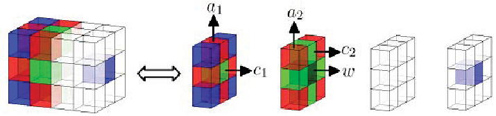
In [2], the authors presented a data-structure (called CubeMap representation) designed to compactly store and quickly manipulate cubical complexes. A similar structure was first introduced in CAPD library [3] for computing cubical homology. In that representation, for each cube (voxel), vertices, edges, squares and the cube itself were encoded in a $3\times 3\times 3$ array with values representing the dimension of each cell (see Fig. 2.c). For a set of voxels, the corresponding array is composed by overlapping copies of arrays of size $3\times 3\times 3$. The CubeMap representation is, in fact, a 3D generalization of the Khalimsky grid, which has already been introduced and extensively used by V. Kovalevsky (e.g. in [9]).

Inspired by that representation scheme, we define a new data-structure, called ExtendedCubeMap representation, that allows to store not only 3D cubical complexes but also the new polyhedral complexes that will be constructed. This new codification is still presented under a 3D array form, also encoding the dimension of the cells that are represented (that is, a 3D grayscale image). In such a structure, the information of boundary relations between represented cells will be extracted by searching for certain structuring elements inside the representation.

An $n$D grayscale image is a map $g:\mathbb{Z}^{n}\to\mathbb{Z}$. Given a point $p\in\mathbb{Z}^{n}$, $g(p)$ is referred to as the color of $p$. A structuring element is also an $n$D grayscale image $b:D_{b}\subseteq\mathbb{Z}^{n}\to\mathbb{Z}$ whose domain contains the origin $o\in D_{b}$. A structuring element will be used to perform a given operation around a certain neighborhood of a point.

An ECM representation of $K$ may not exist and may not be unique (see, for example, Fig. 2.(c,d) which shows two different ECM representations of a single cube together with all its faces). Nevertheless, given a cubical complex $Q(I)$ and the ECM representation $E_{Q}$ of $Q(I)$ given in Prop. 2, the procedures described in the next section will provide a unique polyhedral complex $P(I)$ as well as a unique ECM representation $E_{P}$ of $P(I)$.

Since the map $h_{K}$ is bijective, each cell $\sigma\in K$ is represented by a single point $p_{\sigma}=h^{-1}_{K}(\sigma)\in\mathbb{Z}^{n}$. Moreover, for each $p\in D_{K}$, $g_{K}(p)$ codifies the dimension of the cell in $K$ that $p$ represents (that is, the cell $\sigma=h_{K}(p)$). Finally, observe that the structuring element $b_{\sigma}:D_{\sigma}\to\mathbb{Z}$ associated to a cell $\sigma\in K$ provides a codification of the boundary face relations for $\sigma$. Therefore, within this codification system, the extraction of boundary faces of any cell $\sigma$ can be done by checking if any of the structuring elements of $B_{K}$ fits around the point $p_{\sigma}$ (that is, the point in $D_{K}$ that represents $\sigma$). This last operation could be seen as a morphological erosion of the 3D grayscale image $g_{K}$ by the corresponding structuring element.

Fig. 3 shows an example of a polyhedral complex $K$, the color values in an ECM representation $E_{K}$ of $K$ and the structuring elements (modulo $90-$degree rotations) associated to the cells of $K$.

The following result provides an ECM representation of a cubical complex $Q(I)$ associated to a 3D image $I$. Let $r_{\sigma}$ be the barycenter of $\sigma\in Q(I)$ and $D_{Q}=\{p\in\mathbb{Z}^{3}$ such that $p=4r_{\sigma}$ for some $\sigma\in Q(I)\}$.

Observe that $Q(I)$ is constructed by adding unit cubes $\sigma$ centered at points $r_{\sigma}=(i,j,k)\in\mathbb{Z}^{3}$. Therefore, the possible coordinates of $r_{\mu}$ for the $\ell$-faces $\mu$ of $\sigma$ are:

• •

  $(i\pm\frac{1}{2},j\pm\frac{1}{2},k\pm\frac{1}{2})$ if $\ell=0$;

• •

  $(i,j\pm\frac{1}{2},k\pm\frac{1}{2})$, $(i\pm\frac{1}{2},j,k\pm\frac{1}{2})$ or $(i\pm\frac{1}{2},j\pm\frac{1}{2},k)$, if $\ell=1$;

• •

  $(i\pm\frac{1}{2},j,k)$, $(i,j\pm\frac{1}{2},k)$ or $(i,j,k\pm\frac{1}{2})$, if $\ell=2$;

See Fig. 7 as an example of the color values in the ECM representations $E_{Q}$ for several 3D complete cubical complexes $Q(I)$.

In this section, given the cubical complex $Q(I)$ (associated to a 3D image $I$) and the ECM representation $E_{Q}$ of $Q(I)$ from Prop. 2, we show how to obtain the ECM representation $E_{P}=(h_{P},g_{P},B_{P})$ of a well-composed polyhedral complex $P(I)$ homotopy equivalent to $Q(I)$. The “repairing” process that will be explained below consists of running over all the points $p\in\mathbb{Z}^{3}$ that represent critical vertices $v\in Q(I)$ and accomplishing a color-changing operation by modifying the values of $g_{Q}$ in a neighborhood of $p$. New set of structuring elements, $B_{P}$, is then defined to codify the boundary relations between cells in $P(I)$.

Let $\ell=1,2$. The following sets of points in $\mathbb{Z}^{3}$ will be useful for different descriptions of points inside the ECM representation $E_{P}$:

• •

  $N_{6}^{\ell}=\bigcup_{i=1,2,3}\{(x_{1},x_{2},x_{3})\in\mathbb{Z}^{3}$ s.t. $|x_{i}|=\ell$ and $x_{j}=0$ for $j\neq i\}$.

• •

  $N_{12}^{\ell}=\bigcup_{i=1,2,3}\{(x_{1},x_{2},x_{3})\in\mathbb{Z}^{3}$ s.t. $x_{i}=0$ and $|x_{j}|=\ell$ for $j\neq i\}$.

• •

  $N_{8}^{\ell}=\{(x_{1},x_{2},x_{3})\in\mathbb{Z}^{3}$ s.t. $|x_{i}|=\ell$ for $i=1,2,3\}$.

• •

  $N^{\ell}=\bigcup_{i=1,2,3}\{(x_{1},x_{2},x_{3})\in\mathbb{Z}^{3}$ s.t. $|x_{i}|=\ell$ and $|x_{j}|\leq\ell$ for $j\neq i\}.$

• •

  $N^{\leq\ell}=\{(x_{1},x_{2},x_{3})\in\mathbb{Z}^{3}$ s.t. $|x_{i}|\leq\ell,i=1,2,3\}$.

Finally, for a set $N\subset\mathbb{Z}^{3}$ and a point $p\in\mathbb{Z}^{3}$, let us denote by $N(p)$ the set $\{q+p$ such that $q\in N\}$.

Observe that $N^{\leq 1}=\{o\}\cup N^{1}$ and $N^{\leq 2}=\{o\}\cup N^{1}\cup N^{2}$. In fact, given a point $p\in\mathbb{Z}^{3}$, $N^{\leq\ell}(p)$ is the $(2\ell+1)\times(2\ell+1)\times(2\ell+1)$ block of voxels in $\mathbb{Z}^{3}$ centered at point $p$. If we consider this block as a big cube $C_{p}$ composed by $(2\ell+1)^{3}$ unit cubes, then:

• •

  $N^{\ell}(p)$ are the faces of such a cube $C_{p}$.

• •

  $N^{\ell}_{6}(p)$ are the $6$ endpoints of the $3$ segments with mid-point in $p$, length equal to $2\ell+1$, and parallel to the coordinate axes.

• •

  $N^{\ell}_{12}(p)$ are the (totally $12$) vertices of the $3$ squares centered at $p$, edge-length equal to $2\ell+1$, parallel to the coordinate planes, and whose edges are parallel to coordinate axes.

• •

  $N^{\ell}_{8}(p)$ are the vertices of the cube $C_{p}$.

The following remark ensures that given a point $p\in\mathbb{Z}^{3}$ such that $g_{Q}(p)=0$ (which corresponds to a vertex $v=h_{Q}(p)\in Q(I)$), the modification of the map $g_{Q}$ on the points in $N^{\leq 2}(p)$ only affects to points that either represent cofaces of $v$ or do not represent any cell in $Q(I)$.

See, for example, Fig. 8, which is an example of the values of $g_{Q}$ on the set $N^{\leq 2}(p)$ where $p$ represents a vertex shared by eight cubes in $Q(I)$.

Now, the following method is performed on the ECM representation $E_{Q}$ to construct a new map $g_{P}:\mathbb{Z}^{3}\to\mathbb{Z}$.

Notice that the points $q\in ST_{p}$ representing cubes in $Q(I)$ remain with the same color value, that is, $g_{P}(q)=3=g_{Q}(q)$. The above procedure could be improved by computing the sets $R$ and $\{ST_{p}:p\in R\}$ at once, since the coordinates of the different cofaces of a point $p$ representing a critical vertex in $Q(I)$ are known. For the sake of clarity we have separated the seeking of critical vertices (the set $R$) and their cofaces (the set $ST_{p}$ for each $p$).

References

- [1] Artzy E., Frieder G., Herman G.T.: The theory, design, implementation and evaluation of a three-dimensional surface detection algorithm. Comput. Graphics Image Process. 15, 1–24 (1981)
- [2] Wagner H., Chen C., Vucini E.: Efficient computation of persistent homology for cubical data, in Topological Methods in Data Analysis and Visualization II, Mathematics and Visualization, 91–106 (2012) Proc. of the 4th Workshop on Topology-based Methods in Data Analysis and Visualization (TopoInVis 2011), 2011
- [3] Computer Assisted Proofs in Dynamics: CAPD Homology Library, http://capd.ii.uj.edu.pl.
- [4] Hatcher A.: Algebraic Topology. Cambridge University Press, Cambridge, 2002
- [5] Herman G.T.: Discrete multidimensional Jordan surfaces. CVGIP, Graphical Models Image Process. 54, 507–515 (1992)
- [6] Gonzalez-Diaz, R., Jimenez, M.J., Medrano, B.: Cubical cohomology ring of 3D photographs. Int. J. Imaging Syst. Technol. 21 (1), 76–85 (2011)
- [7] Gonzalez-Diaz R., Umble R., Lamar-Leon J.: Cup products on polyhedral approximations of 3D digital images. In Proc. of the 14th Int. Conf. on Combinatorial image analysis (IWCIA’11). LNCS 6636, 107–119 (2011)
- [8] Gonzalez-Diaz R., Jimenez M.J., Medrano B.: Well-composed cell complexes. In Proc. of the 16th IAPR Int. Conf. on Discrete geometry for computer imagery (DGCI’11). LNCS 6607, 153–162 (2011)
- [9] Kovalevsky V.: Geometry of Locally Finite Spaces. Publishing House, Berlin, Germany (2008)
- [10] Kozlov D.: Combinatorial Algebraic Topology. Algorithms and computation in maths 21, 2008
- [11] Krahnstoever N., Lorenz C.: Computing curvature-adaptive surface triangulations of three-dimensional image data. Vis. Comput. 20 (1), 17–36 (2004)
- [12] Lachaud J. O., Montanvert A.: Continuous analogs of digital boundaries: A topological approach to iso-surfaces. Graphical Models 62, 129–164 (2000)
- [13] Latecki L.J., Eckhardt U., Rosenfeld A.: Well-composed sets. Comput. Vis. Image Underst. 61 (1), 70–83 (1995)
- [14] Latecki L.J.: 3D Well-composed pictures. Graphical Models and Image Processing 59 (3), 164–172 (1997)
- [15] Latecki L.J.: Discrete representation of spatial objects in computer vision. Kluwer Academic, Dordrecht, 1998
- [16] Lorensen, W. E., Cline, H.E.: Marching cubes: A high resolution 3d surface construction algorithm. ACM Computer Graphics 21 (4), 163–169 (1987)
- [17] Marchadier J., Arques D., Michelin S.: Thinning grayscale well-composed images. Pattern Recognit. Lett. 25 (5), 581–590 (2004)
- [18] Stelldinger P., Latecki L.J., Siqueira J.M.: Topological equivalence between a 3D object and the reconstruction of its digital image. IEEE Trans. Pattern Anal. Mach. Intell. 29 (1), 126–140 (2007)
- [19] Stelldinger P.: Image digitization and its influence on shape properties in finite dimensions. IOS Press. 312 (2008)
- [20] Rosenfeld A., Kong T.Y., Wu A.Y.: Digital surfaces. CVGIP, Graphical Models Image Process. 53, 305–312 (1991)
- [21] Siqueira M., Latecki L.J., Tustison N., Gallier J., Gee J.: Topological repairing of 3D digital images. J. Math. Imaging Vis. 30, 249–274 (2008)