A Novel Antenna Selection Scheme for Spatially Correlated Massive MIMO Uplinks with Imperfect Channel Estimation

Multiple-input multiple-output (MIMO) system that employs a large number of antennas, known as massive MIMO systems [1, 2], has been recently proposed as a potential technique, for next generation wireless communication systems [3, 4]. Specifically, in [1], more than 10 fold throughput improvement by the massive MIMO has been suggested to be achievable compared to LTE (Long Term Evolution). Despite such potential, in practice, deployment of massive MIMO systems is hindered by practical challenges. Firstly, there is an inherent problem of spatial correlation among the antennas due to lack of possibility of allowing sufficient spacing among the antennas [2, 5, 6]. Specifically, for the uplink transmission, the antenna correlation could be significant among all the antennas at the base station (BS) side due to the space limitation. In [2], it is shown that correlation among antennas can result in nearly negligible achievable capacity gains. In addition, the channel state information (CSI) is required in order to perform post processing at the receiver side for most of receiver implementations. Prior investigations show that imperfection in channel estimation can significantly degrade the system performance, especially for massive MIMO systems [5, 6].

For the massive MIMO uplinks, the impact of spatial correlation and imperfect channel estimation have been investigated in [1, 2, 5, 6, 7, 8, 9]. More specifically, in [1], it is shown that uplink combining schemes, such as maximum ratio combining (MRC), can have a reasonable performance, with knowledge of CSI for all antenna branches. However, the price to pay for such gain is the significantly increased implementation overhead and the complexity of the transceiver design for massive MIMO systems [10, 11]. In [10], it is argued that cost-efficient antenna selection strategies can be employed to reduce the complexity and overhead of implementation, as well as to effectively maintain a reasonably high performance. Selection combining (SC) for uplink has been extensively studied in the literature such as [12, 13], in the context of conventional MIMO systems. For example, the effect of imperfect channel estimation on the SC systems is investigated in [13], but not for the large scale antenna systems.

An analysis of the MRC in massive MIMO uplinks under imperfect channel estimation is given in [1]. Exploiting sparsity, the work in [14] investigates antenna/relay selection for MIMO channels. However, this work of [14] does not take into account spatial correlation among antennas, as well as the impacts of imperfect CSI acquisition. Considering the spatial correlation and imperfect channel estimation, spatially correlated channel models in [15, 16, 5, 17] are considered as a good approximation for large scale antenna correlation, and channel estimation errors in [18, 5, 17] are applied to effectively model the imperfection caused by the practical channel estimation schemes.

The main contribution of this work is to propose an effective antenna selection combining scheme for spatially correlated single-user massive MIMO uplinks under the imperfect channel estimation, by applying a sparsely structured channel matrix at the BS side. The basic idea is to reduce the effective number of antennas that are used for combining. Consequently, the resulting effective channel matrix becomes sparse, in the sense that the corresponding entries to non-selected antennas are set to zero. This sparse channel matrix can be obtained by some approximation techniques that will be discussed later in this paper. Simulation results indicate that the proposed scheme can significantly reduce implementation complexity and overhead, e.g., it is shown that that only less than half number of antennas are required to achieve a performance level that is comparable to MRC scheme, when the effects of spatial correlation and imperfect channel estimation are taken into account.

The rest of this paper is organised as follows. In Section II, we present the system model. The antenna selection algorithm is proposed in Section III. The proposed scheme is then extended to the spatially correlated channel model with imperfect channel estimation in Section IV. Performance analysis of the proposed scheme and the relevant discussions are given in Section V and VI respectively.

We consider an uplink system with a single user terminal (UT) with a single antenna and one BS with a large number of antennas. The number of antennas at the BS side is $M$, and the received signal vector is represented by

$$\mathbf{y}=\mathbf{h}x+\mathbf{v},$$

(1)

where $\mathbf{h}\in\mathbb{C}^{M\times 1}$ is the channel vector, and $x$ is the transmitted symbol with transmitted power ${\mathbb{E}}\left[xx^{*}\right]=\sigma_{x}^{2}$, where $\left(\cdot\right)^{*}$ denotes complex conjugate. In addition, at the receiver side, we introduce the additive white Gaussian noise (AWGN) vector $\mathbf{v}\in\mathbb{C}^{M\times 1}$, consisting of independent circularly symmetric complex Gaussian random variables with ${\mathbb{E}}\left[\mathbf{v}\mathbf{v}^{H}\right]=\sigma_{v}^{2}\mathbf{I}_{M}$, where $\left(\cdot\right)^{H}$ denotes Hermitian transposition and $\mathbf{I}_{M}$ is the $M\times M$ identity matrix. Hence the signal-to-noise ratio (SNR) can be expressed as $\text{{SNR}}=\sigma_{x}^{2}/\sigma_{v}^{2}$. Throughout this paper, we take into account the spatial correlation among the antennas and imperfect channel estimation, described in the following.

We first consider a single UT equipped with a single antenna at the transmitter side for the uncorrelated i.i.d channel network. In order to realise the multiple receiver antenna selection, here we introduce an antenna selection vector $\mathbf{h}_{s,i}\in\mathbb{C}^{M\times 1}$, which can also be considered as an equalisation vector, due to the fact that each receiver antenna is weighted by a corresponding channel coefficient in the vector $\mathbf{h}_{s,i}$. Considering the expression of received signal in (1), the equalised signal can be given as $\hat{y}$, after we apply the antenna selection vector, as

$$\hat{y}=\mathbf{h}_{s,i}^{H}(\mathbf{h}_{i}x+\mathbf{v}).$$

(8)

Based on the equalised signal structure, the antenna selection can be obtained by minimising the mean squared error (MSE) at the receiver. To achieve this, we define the error signal as

	$\displaystyle e$	$\displaystyle=x-\hat{y}$
		$\displaystyle=x-\mathbf{h}_{s,i}^{H}(\mathbf{h}_{i}x+\mathbf{v}).$		(9)

By exploiting the structure of the error signal, the MSE can be formulated as

	MSE	$\displaystyle\coloneqq E[\left\|e\right\|^{2}]$
		$\displaystyle=\sigma_{x}^{2}-\mathbf{h}_{s,i}^{H}\mathbf{h}_{i}\sigma_{x}^{2}-\sigma_{x}^{2}\mathbf{h}_{i}^{H}\mathbf{h}_{s,i}$
		$\displaystyle\qquad+\mathbf{h}_{s,i}^{H}\sigma_{x}^{2}\mathbf{h}_{i}\mathbf{h}_{i}^{H}\mathbf{h}_{s,i}+\mathbf{h}_{s,i}^{H}\sigma_{v}^{2}\mathbf{I}_{M}\mathbf{h}_{s,i},$		(10)

where “$\coloneqq$” is the definition sign. We then let

		$\displaystyle\tilde{\mathbf{h}}_{i}=\sigma_{x}^{2}\mathbf{h}_{i},$		(11)
		$\displaystyle\mathbf{R}_{i}=\sigma_{x}^{2}\mathbf{h}_{i}\mathbf{h}_{i}^{H}+\sigma_{v}^{2}\mathbf{I}_{M}.$		(12)

Notice that $\mathbf{R}_{i}$ is positive definite, we apply Cholesky decomposition as $\mathbf{R}_{i}=\mathbf{L}_{i}\mathbf{L}_{i}^{H}$ where $\mathbf{L}_{i}$ is one $M\times M$ lower-triangular matrix. The expression of MSE can then be written as

	MSE	$\displaystyle=\sigma_{x}^{2}-\mathbf{h}_{s,i}^{H}\mathbf{L}_{i}\mathbf{L}_{i}^{-1}\tilde{\mathbf{h}}_{i}$
		$\displaystyle\qquad-\tilde{\mathbf{h}}_{i}^{H}\mathbf{L}_{i}^{-H}\mathbf{L}_{i}^{H}\mathbf{h}_{s,i}+\mathbf{h}_{s,i}^{H}\mathbf{L}_{i}\mathbf{L}_{i}^{H}\mathbf{h}_{s,i}$
		$\displaystyle=\sigma_{x}^{2}-\tilde{\mathbf{h}}_{i}^{H}\mathbf{L}_{i}^{-H}\mathbf{L}_{i}^{-1}\tilde{\mathbf{h}}_{i}+\left\|\mathbf{L}_{i}^{H}\mathbf{h}_{s,i}-\mathbf{L}_{i}^{-1}\tilde{\mathbf{h}}_{i}\right\|^{2}_{2}.$		(13)

The only term in (13) related to the antenna selection vector $\mathbf{h}_{s,i}$, which can be further processed, is the last term, i.e., the $L_{2}$ norm (denoted by $\|\cdot\|_{2}$). Such a minimisation problem can be efficiently solved by using sparse approximation algorithms such as the orthogonal matching pursuit (OMP) algorithm, which has been shown that it outperforms the conventional SNR-based selection combining scheme in [14]. More specifically, since the vector $\mathbf{h}_{s,i}$ reflects the receiver antenna selection process, the only non-zero entries of $\mathbf{h}_{s,i}$ correspond to the selected receiver antenna (i.e., $\mathbf{h}_{s,i}$ becomes a sparsely structured vector). Hence, the acquisition of $\mathbf{h}_{s,i}$ transforms to a sparse approximation problem. We formulate this sparse approximation problem by generating a link between the sparse approximation and the MSE optimisation: the objective can be the minimisation of the $L_{2}$ norm, and the measurement dictionary and the target vector are $\mathbf{L}_{i}^{H}$ and $\mathbf{L}_{i}^{-1}\tilde{\mathbf{h}}_{i}$, respectively. In the OMP algorithm, an iterative calculation process is carried out to locate one column vector in the measurement dictionary that is the most correlated vector to the residual vector (which is generally initialised to be the target vector), at each iteration. One locally optimum solution is measured by solving a least-squared problem to update the residual vector. Here, for the sake of simplicity, we highlight the parameters in the algorithm relating to this work. The inputs of the OMP process are the measurement dictionary $\mathbf{L}_{i}^{H}$ and the target vector $\mathbf{L}_{i}^{-1}\tilde{\mathbf{h}}_{i}$, as well as a stopping criterion. Here the stopping criterion is selected as the desired number of iterations for the OMP algorithm, named $K_{s}$. We denote the proposed OMP algorithm as

	$\displaystyle\mathbf{h}_{s,i}$	$\displaystyle=\argmin_{\mathbf{h}_{s,i}|_{\text{{OMP}}}}\left\|\mathbf{L}_{i}^{H}\mathbf{h}_{s,i}-\mathbf{L}_{i}^{-1}\tilde{\mathbf{h}}_{i}\right\|_{2},$
		$\displaystyle\text{{s.t.}}\left\|\mathbf{h}_{s,i}\right\|_{0}=K_{s},$		(14)

where s.t. stands for “subject to”, $\|\cdot\|_{0}$ represents the $L_{0}$ norm, also informally the number of non-zero entries in a vector, and $\mathbf{h}_{s,i}|_{\text{{OMP}}}$ refers to the value of $\mathbf{h}_{s,i}$ calculated by OMP algorithm. Notice that at the end of each iteration, the optimum solution is obtained, corresponding to one selection process of $\mathbf{h}_{s,i}$. Therefore, the stopping criterion $K_{s}$ also indicates the desired number of selected receiver antennas, and multiple antenna selection can be realised by using the sparsely structured antenna selection vector generated by the (14).

In this section, we extend the OMP operation based antenna selection scheme taking into account spatial correlation among the antennas and imperfect channel estimation. Then, in order to use the OMP algorithm in (14) to realise the multiple antenna selection in the spatially correlated channel, we generalise the expression of $\tilde{\mathbf{h}}_{i}$ in (11) and $\mathbf{R}_{i}$ in (12) to

		$\displaystyle\tilde{\mathbf{h}}=\sigma_{x}^{2}\mathbf{h}=\sigma_{x}^{2}\mathbf{\Phi}_{r}^{1/2}\mathbf{h}_{i},$		(15)
		$\displaystyle\mathbf{R}=\sigma_{x}^{2}\mathbf{h}\mathbf{h}^{H}+\sigma_{v}^{2}\mathbf{I}_{M}=\sigma_{x}^{2}\mathbf{\Phi}_{r}^{1/2}\mathbf{h}_{i}\mathbf{h}_{i}^{H}\mathbf{\Phi}_{r}^{H/2}+\sigma_{v}^{2}\mathbf{I}_{M}.$		(16)

The exponential correlation matrix $\mathbf{\Phi}_{r}$ in (16) is accordingly a positive semidefinite matrix [16], so it is necessary to verify the positive definiteness of $\mathbf{R}$ for its availability of Cholesky decomposition. To do so, we introduce the following lemma, and further define the $\mathbf{\Phi}_{r}$ as a symmetric real positive semidefinite matrix (i.e., $\phi\in[0,1)$).

Based on Lemma 1, it can be proved that $\mathbf{R}$ in (16) is positive definite, and the multiple antenna selection with the receiver side spatially correlated channel can be realised, by measuring revised sparse antenna selection vector $\mathbf{h}_{s,c}$, instead of $\mathbf{h}_{s,i}$ in (14), and the relative components in the OMP algorithm. More specifically, we have the generalised $\tilde{\mathbf{h}}$ in (15) and $\mathbf{R}$ in (16), and $\mathbf{L}$ is the $M\times M$ lower-triangular matrix from Cholesky decomposed $\mathbf{R}$. Correspondingly, the measurement dictionary and the target vector become $\mathbf{L}^{H}$ and $\mathbf{L}^{-1}\tilde{\mathbf{h}}$ respectively. We rewrite the structure of $\mathbf{h}_{s,c}$ as

	$\displaystyle\mathbf{h}_{s,c}$	$\displaystyle=\argmin_{\mathbf{h}_{s,c}|_{\text{{OMP}}}}\left\|\mathbf{L}^{H}\mathbf{h}_{s,c}-\mathbf{L}^{-1}\tilde{\mathbf{h}}\right\|_{2},$
		$\displaystyle\text{{s.t.}}\left\|\mathbf{h}_{s,c}\right\|_{0}=K_{s},$		(20)

by considering the same stopping criterion in the OMP operation as (14), i.e., the number of selected antennas. ⁢

Recall the Equation (6) and (7), we now consider the case with imperfect channel estimation. Under the same assumption of a single antenna UT uplink transmission, only the channel estimate vector $\hat{\mathbf{h}}$ is available to the receiver. Generalise the $\tilde{\mathbf{h}}$ and $\mathbf{R}$ to $\tilde{\mathbf{h}}_{e}$ and $\mathbf{R}_{e}$, respectively, which can be given as

$$\tilde{\mathbf{h}}_{e}=\sigma_{x}^{2}\hat{\mathbf{h}}$$

(21)

$$\mathbf{R}_{e}=\sigma_{x}^{2}\hat{\mathbf{h}}\hat{\mathbf{h}}^{H}+\sigma_{v}^{2}\mathbf{I}_{M}.$$

(22)

In a similar way to that provided in Lemma 1, it is evident that the positive definiteness of $\mathbf{R}_{e}$ and the its availability of Cholesky decomposition can be satisfied. We can allocate the parameters for the OMP algorithm with imperfect channel estimation as

	$\displaystyle\mathbf{h}_{s,e}$	$\displaystyle=\argmin_{\mathbf{h}_{s,e}|_{\text{{OMP}}}}\left\|\mathbf{L}_{e}^{H}\mathbf{h}_{s,e}-\mathbf{L}_{e}^{-1}\tilde{\mathbf{h}}_{e}\right\|_{2},$
		$\displaystyle\text{{s.t.}}\left\|\mathbf{h}_{s,e}\right\|_{0}=K_{s},$		(23)

where the $\mathbf{h}_{s,e}$ is the updated version of $\mathbf{h}_{s,c}$ in (20) with consideration of channel estimation error, and $\mathbf{L}_{e}$ is the $M\times M$ lower-triangular matrix generated by the Cholesky decomposition of $\mathbf{R}_{e}$. Again, the stopping criterion is the desired number of selected antennas.

In this section, we compare a series of bit error rate (BER) performances of our proposed scheme with MRC scheme. The system consisting of one single-antenna UT and one BS with a large number of antennas is considered. More specifically, we assume $M=$ 16, 64 or 128. BPSK modulation is applied in our simulations. The effect of sparsity of the antenna selection vector, antenna spatial correlation and imperfect channel estimation can be taken into account by adjusting the value of the parameter $K_{s}$, $\phi$ and $\tau$ in our programme.

Fig. 1 demonstrates the BER performance of the both schemes with different SNR per bit levels. The total number of BS antennas $M$ is set to 64, and correspondingly, we select the half number, i.e., $K_{s}$ equals to 32 out of 64, and more than half number of the BS antennas, i.e., $K_{s}$ is equal to 50 out of 64. Also, we examine several combinations of $\phi$ and $\tau$. It is not surprising to observe that the both schemes are considerably impacted by the high level of $K_{s}$, $\phi$ and $\tau$. However, due to the effective antenna selection process in our algorithms that can minimise the effect of highly correlated channels as well as the channel estimation error during the transmission, our proposed scheme with larger number of selected antennas (i.e., $K_{s}$ = 50) has nearly same performance as MRC, and the gap between the results of MRC and our method with only half antennas selected is fairly negligible. Notice that we show the case with high levels of antenna correlation and channel estimation error (e.g., $\phi$ and $\tau$ equal to 0.6 or even 0.8). In fact, such highly correlated channels can be experienced in our system since the very large BS antenna equipped. In addition, the high level of channel estimation error can be certainly introduced, due to the realistic transmission conditions such as limited feedback and high mobility of UT.

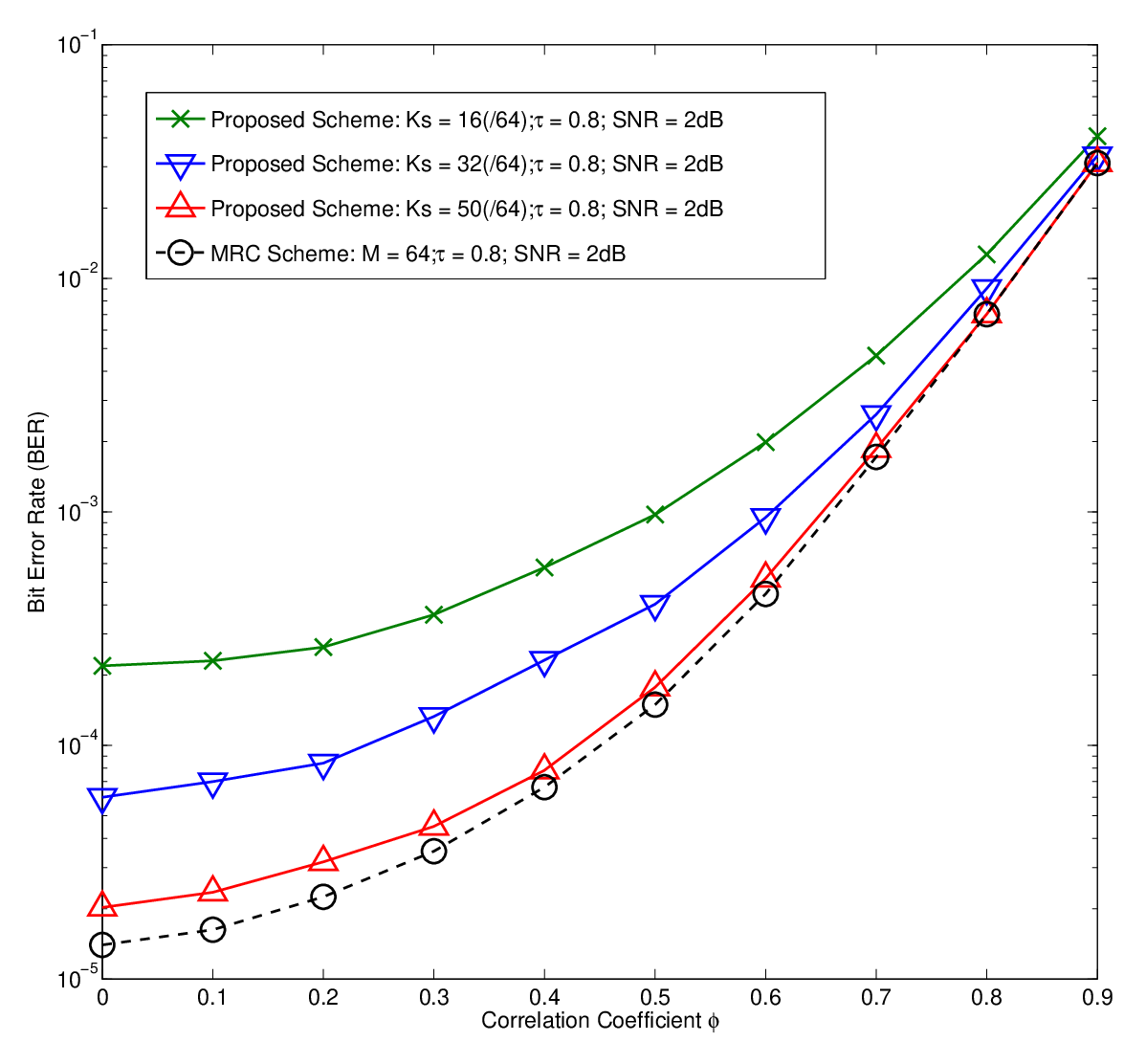
After the general observation of the performance in Fig. 1, now we focus on the effect of different combinations of $\tau$ and $\phi$, and the required number of selected antennas, shown in Fig. 2 and Fig. 3 respectively. First, Fig. 2 illustrates the BER performance of the case, with $M$ = 64, $K_{s}$ = 16, 32 or 50, and $\tau$ = 0.8, by viewing a different aspect from Fig. 1, i.e., with different levels of $\phi$ and in the low SNR regime (SNR = 2dB). It is shown that our scheme has very similar performance with MRC, especially in the high region of $\phi$. In order to take a closer look of the performance with lower $\tau$, in Fig. 3, we choose a lower number of $M$, equals to 16, and select 8 or 10 antennas out of 16. The conclusion holds as well that the compared to the MRC, the performance of our proposed scheme is not degraded by combining only selected antennas, with high levels of $\tau$ and $\phi$ involving. Then, in the interest of high levels of antenna spatial correlation ($\phi$ = 0.8) and imperfect channel estimation ($\tau$ = 0.8), Fig. 4 shows the BER performance versus the number of selected antenna $K_{s}$ of our scheme and MRC, with different levels of SNR. For the high SNR regime, the BER performance of our scheme is closely approached to that of MRC for $M$ = 64 is around 35. For the low SNR regime, approximately measuring, the required number of selected antenna $K_{s}$ is equal to 60 for $M$ = 128, or only 30 for $M$ = 64. It is suggested that when the bad transmission condition introduced in our system, e.g., low SNR regime and high levels of $\phi$ and $\tau$, our proposed scheme has similar, even identical performance as the MRC scheme, with less than half antennas selected, due to the effective selection process designed for different transmission situations.

Throughout this work, we proposed a new antenna selection scheme for the single-user massive MIMO uplink transmission by applying the sparsely structured antenna selection vector, and then generalised our proposed scheme with the consideration of spatial correlation and imperfect channel estimation. Numerical simulation results show that when the severe transmission condition is experienced in our system, such as very low SNR regime, highly correlated channel and considerable estimation error, our proposed scheme has closely approached performance as the well-adopted MRC scheme, but requiring few selected antennas, due to the effective selection process by applying the sparsely structured antenna selection vector, which can significantly reduce the implementation overhead.⁢

Furthermore, due to space limitations, we present our system model here as single user systems, and it is being considered to emphasise upon MU-MIMO in the journal version of this work, e.g., the extension to a single-cell multiuser scenario can be achieved by considering that users independently transmit data to the base station.

This work has been done within joint project, supported by Huawei Tech. Co., Ltd, China.

References

- [1] T. Marzetta, “Noncooperative Cellular Wireless with Unlimited Numbers of Base Station Antennas,” Wireless Communications, IEEE Transactions on, vol. 9, no. 11, pp. 3590–3600, November 2010.
- [2] F. Rusek, D. Persson, B. K. Lau, E. Larsson, T. Marzetta, O. Edfors, and F. Tufvesson, “Scaling Up MIMO: Opportunities and Challenges with Very Large Arrays,” Signal Processing Magazine, IEEE, vol. 30, no. 1, pp. 40–60, Jan 2013.
- [3] E. Larsson, O. Edfors, F. Tufvesson, and T. Marzetta, “Massive MIMO for next generation wireless systems,” Communications Magazine, IEEE, vol. 52, no. 2, pp. 186–195, February 2014.
- [4] F. Boccardi, J. Heath, R.W., A. Lozano, T. Marzetta, and P. Popovski, “Five disruptive technology directions for 5G,” Communications Magazine, IEEE, vol. 52, no. 2, pp. 74–80, February 2014.
- [5] S. Wagner, R. Couillet, M. Debbah, and D. T. M. Slock, “Large System Analysis of Linear Precoding in Correlated MISO Broadcast Channels Under Limited Feedback,” Information Theory, IEEE Transactions on, vol. 58, no. 7, pp. 4509–4537, 2012.
- [6] J. Hoydis, S. ten Brink, and M. Debbah, “Massive MIMO in the UL/DL of Cellular Networks: How Many Antennas Do We Need?” Selected Areas in Communications, IEEE Journal on, vol. 31, no. 2, pp. 160–171, February 2013.
- [7] H. Ngo, E. Larsson, and T. Marzetta, “The Multicell Multiuser MIMO Uplink with Very Large Antenna Arrays and a Finite-Dimensional Channel,” Communications, IEEE Transactions on, vol. 61, no. 6, pp. 2350–2361, June 2013.
- [8] Z. Gao, L. Dai, and Z. Wang, “Structured compressive sensing based superimposed pilot design in downlink large-scale mimo systems,” Electronics Letters, vol. 50, no. 12, pp. 896–898, June 2014.
- [9] W. Shen, Q. Han, J. Feng, J. Ma, and C. Gao, “Antenna selection in measured massive MIMO channels using convex optimization,” in Vehicular Technology Conference (VTC Spring), 2015 IEEE 81st, 2015.
- [10] B. M. Lee, J. Choi, J. Bang, and B.-C. Kang, “An energy efficient antenna selection for large scale green MIMO systems,” in Circuits and Systems (ISCAS), 2013 IEEE International Symposium on, May 2013, pp. 950–953.
- [11] X. Gao, O. Edfors, J. Liu, and F. Tufvesson, “Antenna selection in measured massive MIMO channels using convex optimization,” in IEEE GLOBECOM 2013 Workshop on Emerging Technologies for LTE-Advanced and Beyond-4G, 2013.
- [12] A. Ghrayeb, “A Survey on Antenna Selection for MIMO Communication Systems,” in Information and Communication Technologies, 2006. ICTTA ’06. 2nd, vol. 2, 2006, pp. 2104–2109.
- [13] W. Li and N. Beaulieu, “Effects of channel-estimation errors on receiver selection-combining schemes for Alamouti MIMO systems with BPSK,” Communications, IEEE Transactions on, vol. 54, no. 1, pp. 169–178, Jan 2006.
- [14] J. Lee and N. Al-Dhahir, “Exploiting Sparsity for Multiple Relay Selection with Relay Gain Control in Large AF Relay Networks,” Wireless Communications Letters, IEEE, vol. 2, no. 3, pp. 347–350, 2013.
- [15] S. Chatzinotas, M. Imran, and R. Hoshyar, “On the multicell processing capacity of the cellular MIMO uplink channel in correlated Rayleigh fading environment,” Wireless Communications, IEEE Transactions on, vol. 8, no. 7, pp. 3704–3715, 2009.
- [16] J. Zhang, C.-K. Wen, S. Jin, X. Gao, and K.-K. Wong, “On Capacity of Large-Scale MIMO Multiple Access Channels with Distributed Sets of Correlated Antennas,” Selected Areas in Communications, IEEE Journal on, vol. 31, no. 2, pp. 133–148, February 2013.
- [17] L. Musavian and S. Aissa, “On the achievable sum-rate of correlated MIMO multiple access channel with imperfect channel estimation,” Wireless Communications, IEEE Transactions on, vol. 7, no. 7, pp. 2549–2559, July 2008.
- [18] B. Nosrat-Makouei, J. Andrews, and R. Heath, “MIMO Interference Alignment Over Correlated Channels With Imperfect CSI,” Signal Processing, IEEE Transactions on, vol. 59, no. 6, pp. 2783–2794, 2011.