Embedding multidimensional grids into optimal hypercubes
Abstract
Let and be graphs, with , and a one to one map of their vertices. Let , where is the distance between vertices and of , defined as the minimum number of edges in any path of joining and . Thus is the maximum “stretch” experienced by any edge of under the map . Now let = , over all such maps .
The parameter is a generalization of the classic and much studied “bandwidth” of , defined as , where is the path on points and . In this paper, we study the case when is the -dimensional grid with side lengths , and , , is the hypercube of smallest dimension having at least as many points as . Our main result is that
provided all side lengths of are greater than some fixed constant. For such , this improves on previous results giving the upper bound on the right hand side. Our methods include an application of Knuth’s result on two-way rounding and the use of spanning regular cyclic caterpillars in the hypercube.
1 Introduction
a)
b)
c)
2 The -dimensional mapping
Recall the 2-dimensional grid , with and sufficiently large. In this section we construct a map , where . This will imply that , and additional work will show that has low dilation. This map will be the first step in an inductive process leading to an embedding , and is inspired by the embedding in [9] previously mentioned.
We will need the following notation. Let denote the infinite 2-dimensional grid having rows, so the vertex and edge sets of are , and . We let denote the subset of vertices of with , and refer to this subset “chain ”, or the “’ chain” of .
Now let . We can view as a subset of by the natural correspondence defined as follows. For any vertex of , let , where . To see the action of , let be the subset of consisting of vertices with , . Then maps the points of to the first points of in lexicographic order; that is, if and are two points of , then and if and only if at the smallest index where we have . Recall now the ordering , , of -pages defined at the end of the last section. Then for any and , is the subset of points in given by .
Our method in this section is to first construct a map a low dilation . We then obtain the desired as the composition . For the rest of this section we literally identify any point with , dropping further references to itself. Thus, once is constructed, our map will henceforth be viewed as the restriction of to (under the identification ).
Examples of of , on and , are illustrated in Figure 1 and Figure 2 below. The reader may wish to consult these figures now, and also as we proceed further in this section.


To begin the description of , let positive integers and be given. Then will map either or points of chain to (which recall is column of ). We encode this information by defining a matrix having rows and infinitely many columns indexed by the positive integers, where (resp. ) means that has (resp. ) image points in under the map . In the first case these image points are successive in .
Define the first column of by
For , let the ’th column of be the -fold circular shift downwards of the first column of ; that is, for , where the row index is viewed modulo . Thus is just a circulant matrix whose columns are obtained by successive downward shifts of the first column. We will see that the set of ’s in each column or row of is evenly distributed in a sense that will be described in the lemma which follows.
Lemma 2.1
The matrix has the following properties.
(a) The sum of entries in any column of is .
(b) The sum of any consecutive entries in any row or column of is either or , where .
Proof. For (a), it suffices to prove the claim for column of , since any other column of is just a circular shift of column . This column sum is , which telescopes to .
Consider (b). From the circulant property of and the constant column sum property from part (a), it suffices to prove this claim for any sum of consecutive (mod ) entries in column , say a telescoping sum of the form
Now letting and , we see that this sum is But this difference is either or for any two nonnegative and . Hence the sum is or as claimed.
The basic idea in constructing is to fill out with images under column by column of in increasing column index. For any fixed column of , say the ’th column , we proceed down that column mapping points of in nondecreasing chain index. Each chain will occupy (under the map f) either point or successive points of , depending on whether or respectively.
The construction of follows. For , we let .
Construction of the map
1.The images of in are given as follows.
(1a) Certain points of are mapped to as follows.
If , then and
If , then , , and .
(1b) For to
begin
Assume inductively that for an integer . Certain points of are mapped to as follows.
If , then , and .
If , then , , and .
If , then go to step 2.
end
2. For , the images of in are given inductively as follows.
For to (for sufficiently large)
begin
Suppose inductively that every point of has been defined as an image under . Suppose also that for each , we have for suitable integers , with .
For to
begin
Suppose inductively that is an initial segment of , say given by , where for all .
Certain points of are mapped to as follows.
(2a) If , then , and .
(2b) If , then
(2b1) If is odd, then , , and .
(2b2) If is even, then , , and .
end
end
Recall that the map is illustrated in Figure 1.
Toward analyzing this construction, let . With the goal of showing (in the theorem which follows) that , we wish to analyze . Let be the set of the first points of chain . Now by steps 2a and 2b, contributes either one point or two successive points to any column , depending on whether or respectively, and hence contributes exactly points to . Thus letting , we have . So let be the subgraph of induced by . The next theorem gives various properties of , including .
Finally, we define as the restriction of to the subgraph of . In Figure 2 we illustrate part of for for some . Each -page of is isomorphic to , and the images , , are shown in detail with dividers separating the images of successive -pages. Near these dividers, in each chain of each -page we have placed a box around the image its first point in that -page . For example, under the letter and near the second divider are found three boxed points, these representing the images of the first points in each of the three chains of the third -page . There are four -pages of in each -page of , and we indicate the image of the first -page, consisting of . The beginning of and of are also illustrated at the far right.
Theorem 2.2
The map constructed above has the following properties. We let , let (as in Lemma 2.1b), , and let be the subgraph of induced by .
(a) For each and , or , depending on whether or respectively. Further, if , then consists of two successive points of . Also, is monotone in the sense that for each and .
(b) Let . Then is an initial segment, say , of , with .
(c) For with , let be let be the number of points of mapped to columns through of , so . Then for any we have or , and .
(d) For any we have . Also with as in (b), for any we have .
(e) .
(f) , and .
(g) For any , , and we have .
(h) For any , , and we have .
(i) Suppose that . Then and .
We omit the involved but straightforward proof of this theorem here, and give it in the appendix following the paper. The properties listed above are in any case fairly natural to see, and can be easily verified in Figures 1 and 2.
The following corollary will be used later in proving our dilation bound and the containment . Its proof appears in the appendix.
Corollary 2.3
Let and be adjacent points of . The map constructed above has the following properties.
(a) , and .
(b) .
(c)
(d) Let and be segments of consecutive points on chains and respectively, , where possibly . Let and be the number of columns of spanned by and respectively. The .
(e) Let . Then and .
3 The idea of the general construction, with examples
In this section we give the idea behind our general construction, saving detailed descriptions and proofs of validity for later sections.
The overall plan is to construct a series of maps , , , of which the first, , is given in section 2. The final map gives the basic geometry of our construction, and a relabeling of points of with hypercube addresses gives the final embedding , where . We construct the maps inductively, letting be the composition , as described below. Recall the notation .
Now is an “inflation” map which spreads out the image “evenly” in by successively “skipping over” certain carefully chosen -levels of that are designated “blank”. We let be the set of points lying in nonblank -levels (i.e. levels not designated “blank”) of . We stipulate that . The number of successive -sections in the range of is the same as the number of -pages in , both equalling , and we associate each with in a sense to be made clear below. Define as follows. If , then we let , where is the common -coordinate in the ’th nonblank -level of . The quantity and distribution of blank levels within will be such that for each , the subgraph of has barely sufficient nonblank levels to host . In effect, we want barely sufficient nonblank volume in as in for . We can express this condition as follows. Let be the number of designated blank -levels in section . Observing that for any , and that each -level of has size , and that each section consists of many disjoint -levels, we get
| (1) |
for each .
Next the map “stacks” the sets , , over a single section as follows. Let , . Then we define , where (mod ), , and for (mod . Observe that is defined on , and hence not defined on points in blank -levels of . Nevertheless, we write for for brevity, despite the possibility that contains designated blank -levels whose points are therefore not in the domain of . Note also that since and , we can view the projection as the point of equivalent to .
For a fixed point , we view the set of images under of the form , , as a stack extending into the ’st dimension addressed by . Thus each point of becomes the address of such a stack. As just observed, the points in blank -levels of make no contribution under the map to the aforementioned stacks. So the distribution of blank -levels mod determines the heights of these stacks. The blank levels will be chosen by a kind of evenly balanced distribution mod so as to ensure that the these stack heights are nearly equal.
Letting , we illustrate this process by outlining the construction of from . Noting that and , we use the sections in given by , .
Step 1: Start with the map given in section 2.
Step 2: Designate certain columns in as “blank”, and make the image “skip over” the blank columns in succession as they are encountered left to right (i.e. encountered in increasing column index). The skipping is done by the map defined as follows. If , then let , where is the ’th nonblank column of , counting from the left.
In the first column of Figure 3 we see , where we have separated the four sections of for illustration. The blank columns have been shaded in the figure, so these columns contain no points of . On comparing with Figure 2, we see that is indeed obtained from by skipping over the designated blank columns. Each -section is the host for the -page of , with the possible exception of the images of first points of these -pages, these being indicated by boxes as in Figure 2.

We choose which columns of will be blank, with the following objectives in mind.
(a) We spread out the image so that (as explained above) for each , the subgraph induced by the first sections of has barely enough nonblank columns to host the image of the first many -pages of . As a consequence, each image lies in its own unique section , apart from boundary conditions occurring in the last nonblank column of that , as illustrated in the first column of Figure 3. For each , has just enough nonblank columns ( in , in , in , and in ) to host . The condition (1) with then gives for each . The sequence can be found inductively to be , , , and , and these numbers of blank columns are shown in each of the four sections respectively in that figure .
(b) We wish to ensure that the various images (each mostly contained in its own section ) are coordinated. Specifically, for each , say with and , we want the absolute difference of column indices to be small mod (noting that is the number of columns in any one section ). This condition helps keep the dilation of our final embedding small.
(c) The assignment of blank columns, over all sections of , , is evenly distributed mod , in a sense to be made precise below. This condition allows us to stack the sections on top of each other, over a single section , so that stack addresses in have roughly equal stack heights. Step 3 below explains this further. In the first column of Figure 3, note that each congruence class mod has been selected either once or twice, over all four sections, for a blank column.
Step 3: Finally we stack the sections on top of each other, in order of increasing , over a single section . That is; for each point , the stacking map acts by , where (mod ), , and (mod . As above, we view as the address in of the stack on which has been placed by , and is the ’th point up on this stack. Let be the resulting composition . Again as above, is defined on no point of lying in a designated blank column. Observe that since the image is contained in a collection of stacks addressed by , we can view as previously described, namely, as a map , where is the maximum height of any of these stacks. In this example .
See
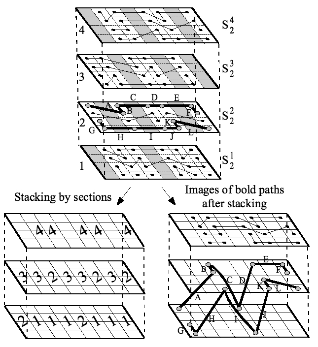
The goals described in step 2 (and elaborated in step 3) can be formulated as combinatorial conditions to be satisfied by the designation of blank columns. It will be convenient to define a matrix having rows, one for each section , and columns, one for each column in any section . We let if column in section (which recall is column in ) is blank, and if that column is nonblank. Since is the number of blank columns in , we must have row sums given by
| (2) |
Consider now the contribution to any stack in from by the stacking map , with the goals of step 2c and step 3 in mind. So for any stack address , let , the set of points in the stack addressed by coming (under the map ) from . Now take any , noting that this condition implies , with (mod , and that column is nonblank. Then we see that the stack height is related to the number of zeros in column and rows through of the matrix . So to keep stack heights nearly equal over all stack addresses , we will require that this number of zeros is nearly the same over all columns in . So in turn we require an evenly balanced distribution of blank columns mod given by
| (3) |
for any .
Next consider the goal in step (2b) of keeping the differences small for , say with and . By Theorem 2.2g, we have the small difference . Let be the number of blank columns in preceding the column, call it , containing , and similarly the corresponding number replacing by and by . Each column counted by pushes the image one more column to the right in , with a similar statement for . Hence the goal would be to keep small. Since each blank column corresponds to a in , we see that each of and is just an initial row sum in (row for and row for ). Thus we want to keep the differences between corresponding initial row sums in small. It will suffice for our purposes to have
| (4) |
for any , , .
We will see that the sequence defined by (1) has, for fixed , the solution satisfying for all . Hence we can view the execution of our plan in steps 1-3, in effect the designation of blank columns, as relying on the construction of a matrix with given row sums differing by at most (from the previous remark and (2)), and having balanced initial column and row sums (from (3) and (4)).
The corresponding requirements for higher dimensions can now be stated as follows. We return to the construction of from as the composition . Recall that there are sections , , and each section has many -levels. So let be the , matrix (analogous to ) defined by if the ’th -level of (that is, level ) is blank, and otherwise. Then the analogues of the relations (2 - 4) become
| (5) |
for ,
| (6) |
for , ,
| (7) |
for , .
Relation (5) says that there are many blank -levels in . Relation (6) says that the blank -levels are uniformly distributed mod , in order to ensure balanced stack heights under the map for stacks addressed by . Finally (7) will imply (after some work) that is small for any , with and , . This will keep the dilation low.
So with motivation similar to the case , in the general case we are similarly reduced to the construction of a matrix with given row sums (with values inductively computed using (1)) differing by at most , and balanced initial column and row sums as required in (6) and (7). We will construct such a matrix in the next section.
Finally, letting we illustrate the construction of , , in a higher dimension.
We must first build , with . For this observe that , so there will be sections, each still of the form . The sequence , , defined by (1) (still with and ) can be calculated inductively to be . A balanced distribution of blank columns among the sections , , satisfying (1) - (4) is given by the matrix shown in the table alias “blank matrices”. Starting then from given in the previous section, we can now define the map which “skips” over the given blank columns as was done in the previous example. The blank columns among the first sections , (as dictated by the first rows of the matrix), are illustrated in the bottom row of Figure 3. The blank columns among the remaining sections , , (dictated by the last rows of the matrix) are now illustrated in middle and top rows of Figure 3. We continue to put boxes around the images of first points of chains in each -page.
We then apply the stacking map as defined above. One can verify that the maximum stack height over all stack addresses is . This can be done by checking that the maximum number of ’s in any column of is , or by seeing that when the sections are stacked in succession over , every stack address (which is just one of the cells in ) has at most points in nonblank columns of corresponding to it, as explained below and illustrated in the figures.
In Figure 5 we show the result of stacking the first sections , , and also stacking all sections , , onto . In the right hand figure, for each stack address , we show which image sets , , contribute points to , while in the left hand figure we illustrate the same thing with restricted to . For example one can check in the right figure that for any stack address , , the indices yielding such contributions are in order of increasing stack height. The resulting stack height is . By contrast, for any stack address , , the section indices thusly contributing to are in order of increasing stack height, and the resulting stack height is .
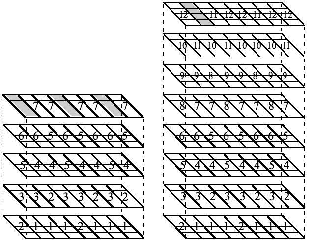
A more detailed look at the members of various stacks addressed by is given in Figure 6. Here we identify the individual points such that belongs to stack addresses in columns and of . For example, consider the members of , consisting of those images with first two coordinates for which lie in the first seven sections , . In this figure we identify the members of this stack by their corresponding points , and find these to be , and , listed in order of increasing stack height.
Now to construct , observe that and , so and for each . Since , we get by (1) the sequence , , and . A balanced distribution of blank -levels among the sections satisfying (1) together with (5) - (7) is given by the matrix given in the lower right of figure alias “blank matrices”. We then apply the map , which inflates by skipping over the designated blank -levels.
The result is represented in the left side of Figure 7 as the set of sections , , each having four -levels, with blank -levels shaded. Now we apply the stacking map , which stacks each of the sets , , in succession onto as defined previously. One can check that the maximum stack height over all stack addresses is , again either by checking that each column of has at most (in fact exactly) zeros, or by seeing in Figure 7 that each of the stack addresses in receives at most points under the map . In the remainder of Figure 7 we illustrate the stacking map in stages. First is stacked on top of , with the result that of the stack addresses (those lying in levels and of ) so far have -dimensional stack height 2 (i.e. for these ), while of the stack addresses (those lying in levels and of ) so far have -dimensional stack height 1 (i.e. for these ). Next, is stacked on top of the previous stacking, so that now every stack address has -dimensional stack height (i.e. for all ).
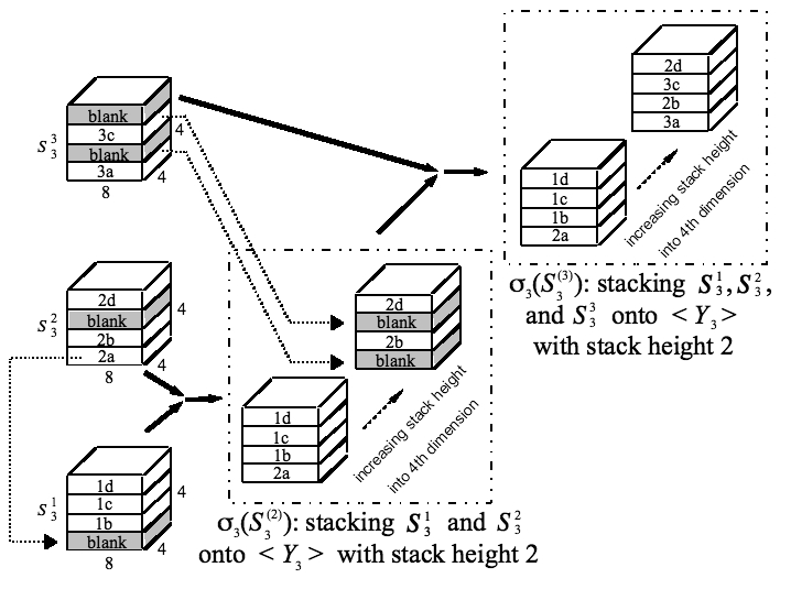
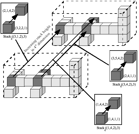
Consider the final result illustrated in the upper right of Figure 7. In that result, let us focus on the stack addresses with , , , these lying in the second -level of (because ). The sets , , contributing points to any such stack satisfy or , realized for by (the latter being the second 2-level of , and for by (the latter being the second 2-level of .
In Figure 8 we look in detail at the individual stacks , , and . For example, the members of are the two images , indicated by their preimages which are and in increasing order of stack height.
4 Tools for the general construction
In this section we develop two tools in our general construction. These are
(1) the designation of blank levels in sections , , and
(2) the construction of an integer labeling of the vertices of any hypercube such that for any reasonably long interval of successive label values, any two vertices
whose labels lie in that interval are at fairly small hypercube distance.
These tools will be combined in the succeeding section to form the embedding
, where
is an arbitrary -dimensional grid.
4.1 The Construction of Blank Levels
In this subsection we describe, for each , , the sequence , , where is the number of -levels of which will be designated blank under the map . We then show that this sequence satisfies property (1) from the overview. That is, for each , we show that has just enough nonblank levels to contain . Finally, we construct for each the actual set of many -levels in that are designated blank, and show that the necessary properties (5)-(7) are satisfied. This construction is based on a theorem of Knuth on simultaneous roundings of sequences.
Define for each our sequence , with , by
where .
Our next lemma shows that these sequences satisfy (1).
Lemma 4.1
Let . Then the sequence , , and , defined above satisfies . In particular, the number of nonblank -levels in is .
Proof. The indicated sum will telescope, and note also that is an integer. Thus . The result follows.
We proceed now to the specification of the many levels in that are designated blank and satisfying the balance properties we required in the overview. For this, we will need the following theorem of Knuth [18].
Let be a sequence of reals, and a permutation of . Let and be the partial sums for these two independent orderings of the ’s. Consider a rounding of the ’s; that is, a designation of integers satisfying for . Now let the corresponding partial sums be and . We say that a rounding of the ’s is consistent with the original sequence (resp. with the permuted sequence under ) if (resp. ) for each . We also say that the rounding is a two-way rounding if it is consistent with both the original sequence and the permuted sequence under .
Theorem 4.2
[18] For any finite sequence of reals and any permutation of , there is a two-way rounding of the sequence relative to .
The existence of two-way roundings was earlier shown by Spencer in [25] by probabilistic methods, as a corollary to more general results on the discrepancy of set systems [22]. Knuth’s network flow based proof, which we omit here, has the advantages that it is constructive and yields improved error bounds.
As a consequence of Knuth’s theorem, we obtain the following theorem (see [11] and [12]) on roundings of matrices which are consistent with respect to all initial row and column sums. We give its short proof for completeness. This extends the rounding lemma of Baranyai ([4]) giving such consistency with respect to all row sums, to all column sums, and to the whole matrix. Additional results on roundings of matrices, including extensions of previous work, applications to digital halftoning, and improved running time and error bounds in implementation can be found in the work of Doerr (see [10], [11], and [12] among others), and Asano (see [1] and [2]).
Theorem 4.3
Let be an matrix with for all and . Then there exists an , , “rounding” matrix of satisfying the following properties.
(a) For each and , , , we have .
(b) For each and , , , we have .
(c) .
Proof. For the most part we paraphrase proofs in [11] and [12]. First consider parts (a) and (b). We construct an matrix from which has integral row and column sums by appending to each row and each column a last entry (possibly ) just large enough to make that row or column have an integer sum. Specifically, let for and , and then for , and for , and . Then has integral row and column sums.
Consider now the following two orderings of the entries of . First we order these entries by “row-major” order; that is, first the entries of row then those of row , etc., until row , and within any row place ahead of iff . Similarly consider the “column-major” order where we place before iff either , or and .
Now apply Knuth’s theorem to obtain a two-way rounding matrix relative to these two orders. Now since every row and column sum of is already an integer, we get for any , and for . Thus taking suitable partial sums in the row major order we get initial row sum estimates for any fixed and . Similarly suitable partial sums in column major order yield for any fixed and . Finally, let be the submatrix of with and . Then recalling that for such and , we get parts (a) and (b) of the theorem.
For (c), let , , and , noting that these three quantities are all since each row or column sum in is integral. Then .
The setting in which we apply Theorem 4.3 is as follows. Let be an integer sequence with or for some integer , and let be a positive integer satisfying . Define the matrix as follows. For each fixed row index , , let for all , . Thus every row of has constant entries. For some rows this constant is while for others it is , and row of has row sum . Now let be an , rounding matrix of as guaranteed to exist by Theorem 4.3. For suitably chosen integers and integer sequence determined by the construction in the next section, this will yield the matrices previously described that encode which -levels of will be designated blank. This has certain balance properties described in the following theorem.
Theorem 4.4
Let be an integer sequence with or for all . Further let be a positive integer with . Then the , rounding matrix of Theorem 4.3 has the following properties.
(a) for any , .
(b) for any , , .
(c) for any , , .
Proof. For part (a), note that the ’ row of has the integer as its sum. Then (a) follows from Theorem 4.3a on taking .
For (b), observe that for any , the sequences of the first entries in any two columns, say and , of are identical. So for any and . Thus by Theorem 4.3b, and are roundings of the same quantity, and hence can differ by at most , proving (b).
For (c), recall that any two rows and of are either identical, or one has constant entries and the other constant entries . So the maximum difference between any two initial row sums of occurs in the second possibility, and in that case the difference we get is . By Theorem 4.3c the initial row sums and of are roundings of the corresponding initial row sums in . Since the latter sums differ by less than , part (c) follows, where the upper bound of is achieved when there is an integer strictly between the corresponding initial row sums in .
Let denote the ’th row of matrix . For any two integers and , , we will later need to bound the column difference between the ’th zero from the left in and the ’th zero from the left in as a function of independent of and . Toward this end, let be the column index of the ’th zero from the left in row of ; that is, .
Now let be the number of zeros in row of . As a convenience, we extend the definition of , even when , by letting , where is the minimum integer for which , with . That is, is the column index of the ’th zero, counting from the first zero in in row major order of zeros.
Corollary 4.5
Let , and let be as just defined. Then the matrix has the following properties.
(a) For and , we have .
(b) For any , , and integers and we have .
(c) For any , , and integers and we have .
Proof. For part (a), let and . Then because is a rounding of (as in Theorem 4.3a) we have , and . So we have , as required.
For part (b), let be the number of zeros in the coordinates of row of for any positive integer . Then using part (a) and we get . Hence we have provided that . Since , the last inequality is in turn satisfied if , and for this it suffices to take independent of and .
Consider now part (c). By Theorem 4.4c we have . So using part (b) of this theorem we get , as required.
4.2 An Integer Labeling of Hypercubes
In this subsection we construct an ordering of the vertices of such that for any interval of roughly consecutive points in , every two points in that interval satisfy . This labeling is based on the existence of certain spanning subgraphs of hypercubes of suitable dimension defined as follows. Define a cyclic caterpillar as a graph such that the removal of all leaves of results in a cycle for some integer . A cyclic caterpillar is r-regular if each vertex of its cycle subgraph has exactly neighboring leaves not on the cycle. Denote such an -regular cyclic caterpillar by .
We are interested in finding spanning subgraphs of the form of hypercubes. Clearly if spans , then , so must be a power of . Papers on this subject include [7], [13], and [16], while [3] examines the general question of finding short dominating cycles or paths in the hypercube. Now [7] contains the following result.
Theorem 4.6
[Corollary 5.8 in [7]] There exists a spanning cyclic regular caterpillar of provided that and .
From this we easily obtain the following.
Corollary 4.7
Suppose and for an integer . Then contains a spanning cyclic -regular caterpillar .
Proof. Recall that is the cartesian product . Hence if contains a spanning subgraph , then contains a spanning subgraph . The corollary follows by induction on .
We can now construct our desired labeling of hypercubes of sufficiently large dimension.
Corollary 4.8
(a) Let be positive integers satisfying and . Then there exists a one to one integer labeling such that for any we have , where the indicated difference is read modulo .
(b) Let . Then there exists a one to one integer labeling such that for any we have , where the indicated difference is taken modulo .
Proof. For (a), consider the spanning subgraph of , , from Corollary 4.7. For , let be the vertices of the cycle in indexed by clockwise order around this cycle. Also let be the leaf neighbors of indexed arbitrarily. Now define by letting for , and for fixed and . It is straightforward to see that this labeling has the required property.
For (b), simply apply part (a) with , , and .
5 The general construction
In this section we inductively construct a series of embeddings , , where it will turn out that . At the end we relabel the points of with hypercube addresses coming from , using the inverse of the labeling of Corollary 4.8. The composition of this relabeling with the map yields the final goal of an embedding .
We follow the general plan outlined in section 3, which the reader is encouraged to review for motivation. The new information we have is a formula, just preceding Lemma 4.1, for the sequences satisfying the relation (1). We are now also ready to construct the matrix , motivated in section , by applying Theorem 4.4.
Recall , the set of points lying in nonblank columns of . Similarly we let , the set of points lying in nonblank columns of , and .
5.1 The three dimensional embedding
In this subsection we construct the map for a -dimensional grid . Here we will be able to picture the construction since it takes place in 3-dimensional space. This will hopefully help in understanding the generalization of this construction in higher dimensions, as in the next subsection.
Construction of the map
1. Set . Construct the embedding of section 2.
2. Set , and let .
Construct the matrix from
Theorem 4.4, using the sequence where
.
Now designate ’blank’ columns in the subgraph of as follows.
Designate column of (which is column of ) as being blank if and only if
.
(Comment: The entries of the matrix now automatically satisfy (1) for and (2)-(4),
by Lemma 4.1b).
3. “Inflate” the image by the map given as follows. For any , let , where is the ’th nonblank column from the left in .
4. “Stack” the sets , , successively “over” by the stacking map defined as follows. Take . Let satisfy (mod ), with Now let (mod . Now define
(Comment: Take any . Then , and . Thus we can view as “stacking” each , “over” .)
5. Finally, define as the composition .
5.2 Embeddings of grids of higher dimension
Again set . In this subsection we inductively construct embeddings for . Assume then that we have constructed the required maps for some , .
Our starting point will be . We will use direct analogues and of the inflation map and the stacking map used in constructing from . In particular, will inflate by introducing blank -dimensional levels using a matrix from Theorem 4.4 that encodes which -dimensional levels of will be designated blank. Then a stacking map will stack the sets , , on top of each other over to yield the final image . Thus we may write as the composition , and inductively .
Construction of the map
1. Assume inductively that the map has been constructed. We now operate on to obtain our image .
2. Set , and let .
Construct the matrix from
(as in the paragraph preceding Theorem 4.4), using the sequence where
(Comment: Matrix now automatically satisfy (1) and (5)-(7))
by Corollary 4.5d).
Consider any -level of (which is ; that is level of ), . Designate
this level as being one of two types as follows.
Level of is ’blank’ if , and is ’nonblank’ if .
3. “Inflate” the image by the map given as follows. Take any . Then let
where is the ’th nonblank level in from step .
4. “Stack” the sets , , on top of each other “over” as increases by the stacking map defined as follows. Let , say with . Let be the integer such that is the ’th nonblank -level of .
(a) Express as , , viewing as the column index in matrix of the ’th zero in row of .
(b) Let and (mod ).
Then define
5. Finally define as the composition . In particular, for any , we have .
We introduce notation needed for the next lemma, with continued use of the notation from the construction above. For any integer with , let = min. As explanation, from step 4 of the construction, we see that is the result of stacking sections , , successively on top of by the map . After the first of these sections are stacked, by definition is the maximum number of points mapped by to any given stack addressed by a point of .
We regard the range of , namely with , as a collection of stacks addressed by the points of . Specifically, for any , we let and . So consists of images which project onto in their first coordinates, and such that comes from the first sections of . From the stacking step 4 of the construction, for with fixed , note that the section number of in increases as the height of in increases. That is, if with and , then implies that . In a similar way, the page number of is nondecreasing as we move up the stack. That is, if with and , then implies that . We refer to these properties of stacks as the stack monotonicity and page monotonicity of stacks.
Lemma 5.1
(a) Let , , and . Taking as in step of the above construction, express as as in step of the construction. Then .
(b) For any , if then .
(c) The restriction of to any single section is a one to one map.
(d) Consider with . For any we have or . Moreover, for any , if and lie in the same -level of (equivalently, ), then .
(e) Let , and . Then for we have
(e1) , and , and
(e2) , and .
(f) For we have .
Proof. Consider first part (a). By steps and of the construction and using induction on we get for integers , , as in step for lower dimensions. Further, , again by steps and . So we obtain for . Applying this to , the result follows.
Consider (b). By part (a) we have and for some , with and both defined relative to the matrix . From and Corollary 4.5 we have that max.
For (c), let be distinct points. We will focus on the first (of the ) coordinates of and to show that that , implying of course that . By step 4 of the construction, we have , with a similar expression for , changing ’s to ’s and to for some . If and disagree at one of their first coordinates, then by these formulas we have so we are done. So assume . Since and lie in the same -section, it follows that and lie in the same set of consecutive integer values. So implies that , yielding that .
Next consider (d) and write . By definition of the matrix , for we have if and only if every point of in level , mod , lies in . Thus every stack address with receives a point (by the stacking map ) in for each such that , and receives no such point if (the latter corresponding to blank -levels). This shows that for such as claimed. It also shows that .
Now by Theorem 4.4b, any two sums and for , differ by at most . Hence for any we have . Since by definition the maximum, over all , of is , part d) follows.
We first prove (e1) by induction on . The base case when follows immediately from Theorem 2.2e,f. For the inductive step suppose , and assume the statement true for and all . Now consider the statement for and any .
First note that by Lemma 4.1b we have . So since is one to one, it follows that , and it remains to show that . Suppose to the contrary that . Now , and by part (d) we have or for each . So by the contrary assumption we have for all such , and by part (d) we have for all in at least one -level of . So since each -level of has size , it follows that . On the other hand by induction we have for some . So since is one to one, we have . If , then we reach a contradiction since . Otherwise, we have . So , again contradicting and thus proving . For the rest of (e1), again note that each -level of has size . Thus we have , proving (e1).
For (e2) we prove both and by induction. If , then both statements hold by Theorem 2.2d,e,f. So let be given, and assume inductively that both of these containments hold for in place of . By this assumption we have . Applying the inflation map to both sides, we obtain , since by Lemma 4.1b we see that has the same number of nonblank -levels as does , and preserves the order of these -levels. Now applying to the last containment, and recalling that , we get , the last containment holding by definition of . By (e1), we have , thereby proving . To show , simply apply the last proved containment, using in place of and observing that .
The containments and follow from (since for all ), from part (d), and from the page monotonicity of the stacks. This completes the inductive step, and hence the proof of (e2) and of (e).
By Lemma 4.1b the number of nonblank -levels in is . Also the inflation map preserves the order of -levels (by -coordinate) in . Now using part (e), we obtain part (f).
We can now give the final embedding of into . It is obtained from by interpreting each coordinate of an image as a hypercube point in using the inverse image of the labeling of Corollary 4.8. The details are as follows.
Construction of the map
1. Initialization and the case .
a) Start with the map .
b) If , then define by .
2. Suppose , and construct the maps inductively as follows.
For to , use to construct as in the procedure above.
3. Having obtained the map from step , define the map by
, where for ,
taking and with being the labeling from Corollary 4.8.
6 Analysis of the construction
Our goal in this section is to verify that the embedding constructed in the previous section satisfies and when every is larger than some constant.
We introduce and recall some notation. For a subset , let . Such an is called -full if . We say that point , , is r-missing (or just missing when ) if . Similarly , , is r-missing if . For , recall that we let and . Now define , and call this the ’th “page stack” of . It follows from Lemma 5.1e,f, that .
By Lemma 5.1e1 we have . In the next theorem we will see that the “page stack” heights , , fall within a narrow range so that for a given any two such heights differ by at most . This will lead to the containments and later to our desired bounds on dilation.
Theorem 6.1
Let and .
(a) For every stack address , we have . In particular, all points of lie in the union of the top two levels of .
(b) .
Proof. Consider first part (a), starting with the upper bound. Note that by Lemma 5.1f. So , by definition of . It follows that .
For the lower bound we first treat very small values of and . The statement holds vacuously for and all (where or ), and also for and all by Theorem 2.2e,f. This implies . So suppose and .
By Lemma 5.1f we have . For a stack address , let and . Applying to both sides of the last containment, we see for any that , where is an integer. But we also have , the last inequality holding since is one to one on sections by Lemma 5.1c. Thus or . Now by Lemma 5.1d,e we have or . Therefore . But again since is one to one on sections, we have . Thus , as required. Finally observe that any point of lies in an level , with by what we have just proved. So the second sentence of part (a) follows.
Next consider (b). By part (a) we have . Also by Lemma 5.1e1 we have . Let and . It follows that , so , as required.
We introduce notation for identifying particular -subpages of a given -page. Let be the ’th -subpage of , so . Let be the union of the first many -subpages of ; so that . Similarly let be the ’th nonblank -level of , ordered by increasing -coordinate, and let . For a point , let be the integer such that ; that is, belongs to the ’th nonblank -level of . It follows that if , , then by Lemma 5.1a.
Corollary 6.2
For we have the following.
(a) For each and , we have .
(b) Set , and let min.
(1) .
(2) .
(c) For , suppose and for some and Let and . Then
(d) For , let and .
(1) If , then .
(2) If , then .
(e) Suppose , .
(1) If , then .
(2) If , then .
(f) .
Proof. Consider (a). Since by Lemma 5.1f, it suffices to show that . Recall now that . By Lemma 5.1e1 we have . So by Lemma 4.1b we see that is the number of nonblank levels in . Thus consists of the nonblank levels of . Since by Theorem 6.1a only the top two levels of can possibly contain points not in , it follows that only the top two nonblank levels of , call them and , can possibly contain points not in . Thus . But since for all , these top two nonblank levels , of lie in the last section of . So as desired.
For part (b), set . Since the inflation map preserves the order of levels in , it follows that corresponds under to the topmost levels of . By Theorem 6.1a, the only levels among these levels which could possibly be not -full are and . Further by Theorem 6.1b we have . Again by the correspondence under , it follows that the only nonblank levels of which could possibly be not -full are . Since is just a translation of levels, it preserves inverse images under , so we also have . It follows that , as required.
For part (c), let , and let . Further, set , so is just the size of any single -level of an -section such as . Let = min, and = max. We let either of these two parameters be if the stated intersection is empty. Our approach will be to find a lower bound for and an upper bound for independent of .
We begin with a lower bound for . Recall notation from the proof of part (b). The last many -pages of form , and also constitute the first many -pages of . Hence all but at most points of lie in by Lemma 5.1e1, so Thus intersects at least the first nonblank levels of
NEW STUFF: We seek a lower bound for and an upper bound for , independent of . We use the notation from the proof of part (b). The last many -pages of form , and also constitute the first many -pages of . Hence all but at most points of lie in by Lemma 5.1e1, so Thus intersects at least the first nonblank levels of
NEW STUFF: We give an upper bound for = max. Recall that . Consider the set , having size at most . By part (b) we have , so .
NEW STUFF: Next we give a lower bound for = min.
By part (b), (applied to in place of ) the only levels of
possibly containing points not in are the top two levels of . So we have
. Hence .
For an upper bound on , recall that . Consider the set , having size at most . By part (b) we have .
These bounds also apply to and , only replacing by . So letting and , it follows that , as required.
Consider now part (d). Let and be the stack addresses of the images and ; that is and . By Lemma 5.1d we have . Since is one to one on any section, we know that (resp. ) will be the topmost entry of (resp. ), so , with the same inequality holding for . Part (d1) follows. For (d2), suppose without loss that . Note again that since is one to one we get . Using Lemma 5.1d we then have . Since also by Lemma 5.1d, part (d2) follows.
For (e), observe first that for any we have by part (a) of this corollary. So for any , the points and lie in the same -section or in successive -sections of . Hence (e1) follows directly from part (d1). For (e2), again using we find that and , where . So (e2) follows directly from part (d2).
Consider part (f). Again let , so that . By Lemma 5.1e2 we have , where . Thus, since obviously , we see that is contained in the vertex set of the -dimensional grid . The right side, being a product of paths of lengths powers of summing to , is itself a spanning subgraph of . Thus as required.
We can now proceed to our main theorem, a bound on the dilation bound of our embedding. In the proof we frequently apply Corollary 4.5, where (in the language of its statement) we use relative to some matrix . In each application, the role of in that corollary will be played by a matrix from step 2 of the construction of from (section 5). The value of will change from one application to another. So in the proof which follows, let denote the of the corollary, when in the application we intend to use in the role of . So for example, in applying the Corollary 4.5b with , with the intention of using in the role of , we would conclude that .
Theorem 6.3
Let be an arbitrary -dimensional grid with for each . Then the embedding from section 5.2 satisfies .
Proof. Let and be an arbitrary pair of adjacent points of , and set and for short. Recall that , where is the string of equivalent to under the labeling of Corollary 4.8. It suffices to show for each , , that we have . For then by the definition of just given and Corollary 4.8b we have , so the bound follows immediately. Thus we are reduced to showing that for each .
Let , , be the unique coordinate at which a pair disagree, so . Also let . For any given , the maximum of over all serves as an upper bound for , over all edges . So let be an edge at which this maximum occurs for a given , and refer to this edge simply as since will be understood by context.
We begin with , starting with the case for a bound on . Since , and are corresponding points on successive chains and of . So we have as required, where the next to last inequality follows from Corollary 2.3a. Now suppose . Thus and agree in their first coordinate, and hence can be considered as lying on the same chain of . So by Theorem 2.2h we have .
Now suppose that . If , then again and are corresponding points on successive chains of . Thus by Theorem 2.2g we get . Hence by Lemma 5.1b we get .
If , then and are successive points on the same chain of , so by Corollary 2.3a we have . So again by Corollary 5.1b .
Now suppose , still with . Let be the common second coordinate for and . Then and belong to the same chain of . So they may be viewed as corresponding points belonging to some distinct -pages and of respectively of . Consider the segments and of given by and . We see that (resp. ) is the initial segment of points of the chain in (resp. ), and that and are the last points of these segments. Let and be the number of successive columns of spanned by and respectively. By Corollary 2.3d we have . The columns spanned by (resp. ) are transformed under the inflation map into a corresponding set of (resp. ) successive nonblank columns in . Corollary 2.3e and Lemma 4.1b now imply that each of and , being the transforms of and , begins either in the first nonblank column of its section ( for and for ) or the last nonblank column of its preceding section ( for and for ). The maximum value of (in the notation preceding Corollary 6.2) is then achieved when . In that case transformed segment spanning the greater number of columns begins in the first nonblank column of its section while the transformed segment spanning the lesser number of columns begins in the last nonblank column of its preceding section. So in that case . Now let and . Then by Corollary 5.1a and the remarks immediately preceding Corollary 6.2 we have and . So by Corollary 4.5c with we have .
Next suppose . We argue according to the order relation between and .
Suppose first that . Then and belong to the same -page and successive -pages of . We obtain our bound independent of . Now and belong to the same -section or to successive -sections and , , of by Corollary 6.2a. Applying Corollary 6.2d, in the first case (same -section) we get by part (d1), while in the second case (successive -sections) we get by part (d2). Hence by Lemma 5.1b with and using the more generous second case bound to cover both cases, we get , as required.
Now suppose . Then and are corresponding points in successive -pages. Hence by Corollary 6.2e2 we get . Thus by Lemma 5.1b with we get .
It remains to consider the case . Here and are corresponding points in successive -pages, say and . Consider the -pages containing and , say and for suitable integers and . Since and must also be corresponding points in these -pages, we have (in the notation preceding Corollary 6.2) and for the same integer . As before, let and for brevity. Then by Corollary 6.2c we get . Again applying Lemma 5.1a we have and . So applying Corollary 4.5c with we get , completing the proof.
7 Appendix: Proofs of Theorem 2.2 and Corollary 2.3
Proof of Theorem 2.2: Part (a) follows directly from steps 2a and 2b of the construction of . In part (b), the claim that is an initial segment of follows directly from part (a), step 2 of the construction of , and induction on . The claim on follows from step 2 of this construction on noting that contributes (resp. ) to this sum if (resp. ), where the second to last equality is justified by Lemma 2.1a.
Consider (c). By part (a), is the number of columns , , such that
, while in the remaining columns , , we have . The formula for
follows. Observe also that
by the formula for and Theorem 2.1b.
The same equation
with replaced by
yields the rest of (c).
Part (d) follows from parts(b,c) and Lemma 2.1b. For (e), by part (c) (taking ) and the definition of we see that . So it suffices to show that . We have .
Now consider (f), and recall the notation for the number of -pages in , so in particular . We use the fact that can be identified with the the subgraph of induced by the union of initial segments . For or let , and . We claim that . If not, then , so by (d). It follows that . But this contradicts , proving that . Hence for each we have , implying that by the identification of above. To show , begin by observing from the definition of that . Thus . So one of the terms in the last sum is less than . It follows that and hence by (d). This says that for each , , and hence that for by the monotonicity of from part (a). It follows that , as required.
For (g), we proceed by induction on . The base case is clear since for all . Assume inductively that for some , and let . If , then we are done since or and the same holds for . So suppose without loss of generality that . Then by (c) and by Lemma 2.1. If , then we are done since . So we may assume . If now , then we are done again. So we can assume also that . Then we get , contradicting .
Now consider (h). Set where , , is arbitrary. It suffices to show that must be one of three consecutive integers which depend only on , but not on . By (b), the set is the initial segment of size in . So by Lemma 2.1, is either or . Now consists of either one or two successive points of which immediately follow the point . Hence must be one of the three successive integers , or , proving (h).
Finally consider (i). The proof is based on being a downward shift of (with wraparound) for any . We refer to this property as the “downward shift” property. The assumption says that (viewing subscripts modulo ), by the downward shift property. Hence by part (b) and this same property, we have , since . For the second claim, observe that by the downward shift property. Similarly we have . Therefore , since .
This completes the proof of the theorem.
Proof of Corollary 2.3: As a convenience, we prove these properties with replacing , to facilitate direct reference to the construction above. Of course then inherits these properties since it is a restriction of . For brevity let and .
Consider first part (a). We get by Theorem 2.2a if and are successive points on the same chain, and by Theorem 2.2g otherwise (i.e., if and for some and ). We also get by Theorem 2.2h if and are successive points on the same chain. So we are reduced to showing that when, say, and for some and . Let . If also then since by Theorem 2.2a,b we have that is a set of at most successive points of , it follows that .
So let , noting that then since we have already shown that . We prove the stronger statement that in this case. This will complete the proof of (a), and also yield (b) as a corollary, since .
First we need some terminology. Suppose for some and , and let for some . We will say that is in the (resp. ) state if (resp. ). Now let , say with with , and , be a second such point. We will say that the ordered pair is in state , where each of and is or , if (resp. ) is in state (resp. ). Note for future reference that by step (2b) of the construction, when is even (resp. odd) and , then (resp. ).
Suppose first that , still with and for some and . Further suppose that . We will consider the four possible states of the ordered pair . If the pair is in state then and , while if in state then and , and if in state , then and , all contradictions to Theorem 2.2d. So suppose that is in the state . Then by Theorem 2.2i we have . Suppose first is odd. Then while . Thus , as required. So suppose that is even. Then . So , completing the proof when .
So suppose that . The three states , , and for the pair are immediately eliminated as above by contradicting part (d) of Theorem 2.2, where we omit the details since they are similar to the ones given above in eliminating three of the states. So finally suppose the pair is in state . We reduce ourselves to proving our claim in the case , as follows. Suppose first that , so by part (d) the theorem , since is in the - state. Then since is in the + state we have , as required. Next suppose , so . If also , then , contradicting part (d) of the theorem. So . and hence by part (i) of the theorem . But and imply that and , a contradiction. So we are reduced to the case . If is even, then by the construction , as required. If is odd, then , as required.
It remains to prove when at least one of the two intersections and has size , still with . Suppose first that . Since is by definition the downward shift of , it follows that . So we are reduced to both intersections having size . Then , so using Theorem 2.2d we get , as required.
We can then assume that . Suppose first that while . If , then , as required. So we can assume that , and hence by part (d) of the theorem. We claim that . If not, then , so . Since , we have . Thus , contradicting part (d) of Theorem 2.2. Thus we have . Again since is a unit downward shift of , we get . This implies that , while since . But since by assumption, Theorem 2.2i implies , a contradiction.
So we can suppose that while . If , then , as required. So we can assume , by part (d) of the theorem. If , then , as required. Thus we can suppose that . Hence also by being a downward shift of . Now since . Thus using and part (i) of the theorem. But since , a contradiction.
Finally suppose that . Here the proof of is identical to the proof given in the case when both intersections have size , just replacing in that proof by .
Consider part (c). Since , we see that is a subgraph of the spanning subgraph of . Thus by Theorem 2.2e,f we obtain , as required.
Consider next part (d). As notation, for let be the union of columns through of . Let then and be the sets of columns of spanned by and respectively. Suppose to the contrary that . By symmetry we can assume that .
Let , and let . Now for each we have with the possible exception when or , since in these exceptions possibly is just the second of two points of . So since it follows that . So . Thus by Theorem 2.2c we have . Now , since omits at least the two endpoints of the path . But also , a contradiction.
Finally we prove part (e). The containment in (e) follows from (d) (also from Theorem 2.2e,f. The bound on follows from , since by that containment the set is a proper subset of the column .
References
- [1] T. Asano, T. Matsui, and T. Tokuyama: Optimal Roundings of Sequences and Matrices, Nordic J. Comput. 7 (2000) 241-256.
- [2] T. Asano, N. Katoh, K. Obokata, and T. Tokuyama: Matrix Rounding Under the -Discrepancy Measure and Its Application to Digital Halftoning, SIAM J. Comput. 32 No.6 (2003) 1423-1435.
- [3] U. Blass: Short Dominating Paths and Cycles in the Binary Hypercube, Annals of Combinatorics 5 No. 1 (2001) 51-59.
- [4] Zs. Baranyai: On the Factorization of the Complete Uniform Hypergraph, in Infinite and Finite Sets, Proc. Coll. Keszthely, 1975, Colloquia Math. Soc. János Bolyai A. Hajnal, R. Rado, V.T. Sós (Eds.), Colloquia Math. Soc. János Bolyai 10 North-Holland (1975) 91-108.
- [5] S. Bettayeb, Z. Miller, and I.H. Sudborough: Embedding Grids into Hypercubes, J. Comput. System Sci. 45 No. 3 (1992) 340-366.
- [6] S. Bhatt, F.R.K. Chung, F.T. Leighton, and A. Rosenberg: Efficient Embeddings of Trees in Hypercubes, SIAM J. Comput. 21 No.1 (1992) 151-162.
- [7] R. Caha and V. Koubek: Spanning Regular Caterpillars in Hypercubes, European J. Combinatorics 18 (1997) 249-266.
- [8] Y. Cai, T.H. Lai, and C.C. Lin: Embedding Two-Dimensional Grids into Hypercubes with Dilation and Congestion , Proc. Intern. Conf. on Parallel Processing, Oconomowoc, Wisc., III, (1995) 105-112.
- [9] M.Y. Chan: Embeddings of Grids into Optimal Hypercubes, SIAM J. Comput. 20 No. 5 (1991) 834-864.
- [10] B. Doerr: Matrix Rounding with Respect to Small Submatrices, Random Structures & Algorithms 28 (2006) 107-112.
- [11] B. Doerr, T. Friedrich, C. Klein, R. Osbild: Rounding of Sequences and Matrices, with Applications, Proceedings of the Workshop on Approximation and Online Algorithms (WAOA 2005) T. Erlebach, G. Persiano (Eds.) Vol. 3879 of Lecture Notes in Computer Science, Springer Verlag, (2006) 96-109.
- [12] B. Doerr, T. Friedrich, C. Klein, and R. Osbild: Unbiased Matrix Rounding, Proceedings of the 10th Scandinavian Workshop on Algorithm Theory (SWAT), L. Arge, R. Freivalds (Eds.) Vol. 4059 of Lecture Notes in Computer Science, Springer Verlag, (2006) 102-112.
- [13] T. Dvorak, I. Havel, J-M Laborde, and M. Mollard, Journal of Graph Theory 24 No. 1 (1997) 9-19.
- [14] I. Havel and P. Liebl: Embedding the Polytomic Tree into the -cube, Casopis Pest. Mat. 98 (1973) 307-314.
- [15] I. Havel and J. Moravek: -Valuations of Graphs, Czech. Math. J. 22 (1972) 338-351.
- [16] F. Harary, M. Lewinter, and W. Widulski, Congress. Numer. (19’th Southeastern Conference on Comb., Graph Theory, and Computing) 66 (1988) 103-108.
- [17] Y.M. Kim and T.H. Lai: The Complexity of Congestion-1 Embedding in a Hypercube, J. of Algorithms 12 No. 2 (1991) 246-280.
- [18] D.E. Knuth: Two-Way Rounding, SIAM J. Disc. Math 8 No. 2 (1995) 281-290.
- [19] J. Lee: On the Efficient Simulation of Networks by Hypercube Machines, Ph.D. Dissertation, Dept. of Electrical Engineering and Computer Science, Northwestern University (1990).
- [20] F.T. Leighton: Introduction to Parallel Algorithms and Architectures: Arrays, Trees, Hypercubes, Morgan Kaufman Publishers, San Mateo, CA (1992).
- [21] M. Livingston and Q. Stout: Embeddings in Hypercubes, Mathematics and Computational Modelling 11 (1988) 222-227.
- [22] L. Lovasz, J. Spencer, and K. Vestergombi: Discrepancy of Set Systems and Matrices, European J. of Combin. 7 (1986) 151-160.
- [23] Z. Miller and I.H. Sudborough: Compressing Grids into small Hypercubes. Networks 24 No. 6 (1994) 327-357.
- [24] M Rottger, U. Schroeder: Embedding 2-Dimensional Grids into Optimal Hypercubes with Edge Congestion 1 or 2, Parallel Processing Letters 8 No. 2 (1998) 231-242.
- [25] J. Spencer: Ten Lectures on the Probabilistic Method , CBMS-NSF Regional Conference Series in Applied Mathematics 52 SIAM, Philadelphia (1987) 37-44.
- [26] D.B. West: Introduction to Graph Theory (Second Edition) Prentice Hall (2001).