Acceleration of Type 2 Spicules in the Solar Chromosphere - 2: Viscous Braking and Upper Bounds on Coronal Energy Input
Abstract
A magnetohydrodynamic model is used to determine conditions under which the Lorentz force accelerates plasma to type 2 spicule speeds in the chromosphere. The model generalizes a previous model to include a more realistic pre-spicule state, and the vertical viscous force. Two cases of acceleration under upper chromospheric conditions are considered. The magnetic field strength for these cases is and 25 G. Plasma is accelerated to terminal vertical speeds of 66 and 78 km-s-1 in s, compared with 124 and 397 km-s-1 for the case of zero viscosity. The flows are localized within horizontal diameters and 50 km. The total thermal energy generated by viscous dissipation is times larger than that due to Joule dissipation, but the magnitude of the total cooling due to rarefaction is this energy. Compressive heating dominates during the early phase of acceleration. The maximum energy injected into the corona by type 2 spicules, defined as the energy flux in the upper chromosphere, may largely balance total coronal energy losses in quiet regions, possibly also in coronal holes, but not in active regions. It is proposed that magnetic flux emergence in intergranular regions drives type 2 spicules.
Keywords:
MHD - Sun: chromosphere - stars: chromospheres - Sun: magnetic fields - stars: coronae - Sun: corona1. Introduction
In a review of small scale chromospheric structures, Tsiropoula et al. (2012) point out that the existence of spicules in the chromosphere, eventually identified as mainly vertical supersonic flows, has been inferred from observations for more than 130 years. As spatial and temporal resolution has increased, the observed maximum flow speeds of spicules have increased, and the observed minimum length scales over which these flows are localized orthogonal to their velocity have decreased. This trend is similar to that of observing, and using semi-empirical models to infer the existence of, increasingly stronger magnetic field strengths and total magnetic energy on increasingly smaller horizontal scales in the photosphere (de Wijn et al. 2009; Sánchez Almeida & Martínez González 2011; Stenflo 2012, 2013). These trends can be connected in that Lorentz forces on a given scale can drive flow on that scale. There is no sign that the smallest scales of magnetic fields or supersonic flows in any region of the solar atmosphere are resolved.
These trends suggest that type 2 spicules, observed on the limb and on the disk (as rapid blueshifted excursions - RBE’s) (De Pontieu et al. 2007 a,b,c; Langangen et al. 2008; Rouppe van der Voort et al. 2009; Sekse et al. 2012; De Pontieu et al. 2012; de Wign 2012) are the sub-set of chromospheric flows with the highest speeds , and shortest durations that can be detected with the highest available spatial and temporal resolution of and 5-8 s (van Noort & Rouppe van der Voort 2006; De Pontieu et al. 2007 c; Tavabi et al. 2011; Pereira et al. 2012).
This paper uses a magnetohydrodynamic (MHD) model that improves upon the model in Goodman (2012, henceforth G12) to determine conditions under which flows can be accelerated to vertical speeds comparable to type 2 spicule speeds in the chromosphere. The model in G12 assumes a pre-spicule state without flow, with a constant vertical magnetic field, and neglects the effects of viscosity. The model presented here includes a pre-spicule state with 2 D velocity and magnetic fields, and the viscous force due to HI-HI collisions.
2. The Model
Assume cylindrical coordinates . Let be time. All quantities are independent of , and is height above some to be specified point in the chromosphere. Assume a weakly ionized H plasma with constant temperature . Then , where , and are the pressure, mass density, sound speed, proton mass, and Boltzmann’s constant. Assume and . Here is the pressure scale height, where cm-s-2. Then the vertical pressure gradient and gravitational forces cancel.
Let be the center of mass (bulk flow) velocity. Assume the magnetic field . Include the viscous force due to HI-HI collisions in the momentum equation. For the momentum and mass conservation equations an exact solution for the height dependence of is that it is independent of height. This form of the solution is assumed here, so . The assumed form of the height dependence of , and implies the flow is accelerated by height independent Lorentz and viscous forces per unit mass acting on a vertical column of gas. The current density . It is assumed that .
Under the preceding assumptions, the momentum and mass conservation equations are
| (1) |
| (2) |
| (3) |
| (4) |
Here the dot and prime denote and , and is the viscosity of HI, where is an estimate of the atomic diameter (Mihalas & Mihalas 1984). Here , where is the Bohr radius.
The is now restricted to being sufficiently small to simplify solving the model. This restriction, together with the restriction made above that , is consistent with the observation that the primary acceleration is in the vertical direction. These restrictions prevent the model from reproducing horizontal and torsional flows, with speeds up to km-s-1, exhibited by some type 2 spicules (Sekse et al. 2012; De Pontieu et al. 2012).
Constraints are imposed on to justify omitting the terms involving in the momentum equations (1) and (3). Inspection of those equations indicates the constraints , and should be adequate for the solutions presented in §6. As shown in §3, the constraint on places an upper bound on , which is the characteristic radius within which is confined. Imposing these constraints reduces equations (1) and (3) to
| (5) |
| (6) |
In order that the solution for be finite at it is necessary that the boundary condition be imposed. One more boundary condition is necessary to uniquely determine the solution for . This is chosen as since the observed diameter of type 2 spicules is km. For the solutions in §6, the plasma acceleration, and resistive, viscous, and compressive heating occur almost entirely within a radius km from the origin.
2.1. Accelerating and Compressive Lorentz Forces
If the Lorentz force plays an important role in accelerating spicules then it must be localized on the space and time scales observed to characterize spicules. The vertical Lorentz force is . Here a functional form for is assumed, given by Eq. (7) below, that is localized on time and radial scales and to model the temporal and radial localization of type 2 spicules. As shown below, the assumed form for together with the equations , and determine and , and hence the contribution to the vertical Lorentz force. For the two spicule solutions presented in §6, this is the accelerating Lorentz force in that it drives all of the upward acceleration of the plasma. It does this against a much weaker downward component, , of the vertical Lorentz force present in the background (BG) state. The values of and are chosen so the solutions exhibit a plasma acceleration time, and radial localization of the accelerated plasma consistent with observations. The observations of type 2 spicules referenced in §1 show they have durations s, and characteristic diameters km. In §6, the choice s yields an acceleration time of s to maximum vertical speeds of and 77 km-s-1, and the corresponding choices of and 1.25 km yield flows mainly confined within diameters and 50 km.
is assumed to have the following form.
| (7) |
Here and .
The specification of , and causes the complete MHD model to be over-determined. Consequently, three equations must be omitted from the complete MHD model. The remaining equations determine the solution self-consistently. Here the mass and momentum equations, Faraday’s law, the component of a multi-fluid Ohm’s law, the ideal gas equation of state, and an NLTE Saha equation are used to determine the solution to the model. The energy equation, and the and components of the Ohm’s are omitted from the model, except that the complete Ohm’s law is used to estimate the Joule heating rate.
It follows from that
| (8) |
From it follows that
| (9) |
where .
With respect to , the maximum values of , and are reached at , for which . With respect to , the maximum values of and are reached at , for which . The maximum value of , and hence of is then . Then specifying determines the maximum magnitude of , and determines . Figure 1 shows over the effective time interval of Lorentz force driven acceleration, where is the maximum value of .
2.2. Background (BG) State
This is a state in which . It is determined by , and in that once these quantities are known they determine , and for this state. Equation (2), and imply
| (10) | |||||
| (11) |
where is an arbitrary function of time, specified in §3. For the spicule solutions presented in §6, during the main phase of the acceleration. Such a highly twisted field may be susceptible to the kink instability in the real chromosphere. The specification of the time dependence of and forces the model solutions to be stable. A model driven only by initial and boundary conditions is required to determine the stability of such field configurations in the chromosphere.
The simplifying assumptions in §2 that and cause the component of the momentum equation to reduce to Eq. (2). This causes the BG state to become un-coupled from the spicule in that the BG state influences the spicule acceleration process, but this process does not affect the BG state. In reality, there is bi-directional coupling between the pre-spicule state of the atmosphere, and the subsequent spicule acceleration process. The strength of this coupling is not known. A model that allows for bi-directional coupling, for example one that does not require that , or that and be small in the sense defined in §§2 and 3, is needed to estimate the importance of this coupling. A potentially important effect omitted due to the un-coupling of the spicule from the BG plasma is the distortion of the BG magnetic field due to partial flux freezing, which increases with temperature and degree of ionization.
The model presented here assumes the existence of a current that accelerates plasma through the Lorentz force. The source of this current is not specified. It is proposed here that the source is the emergence of current carrying magnetic flux through the photosphere in inter-granular lanes on scales km. These magnetic structures may rise into the chromosphere with unbalanced Lorentz forces that accelerate plasma as part of the process of relaxation of towards a force free, minimum energy state. Magnetic flux emergence, driven by convection, occurs continuously on inter-granular scales, and as observations have improved, more flux has been observed on increasingly smaller scales (Lites et al. 1996; Orozco Suárez et al. 2007; Lites et al. 2008; Lites 2009). These emerging magnetic structures have or develop a vertical, quasi-cylindrical geometry, similar to the geometry of type 2 spicules. The proposition that magnetic flux emergence drives type 2 spicules is discussed in more detail in §7.
Driving by magnetic reconnection (e.g. Rouppe van der Voort et al. 2009) is unlikely since type 2 spicules are often observed in regions that appear to be unipolar (McIntosh & De Pontieu 2009; Martínez-Sykora et al. 2011), and since in reconnection an upward jet is expected to be accompanied by a downward jet, whereas there do not appear to be observations of type 2 spicules as multi-jet phenomena. The model presented here includes a radial Lorentz force that compresses the plasma, increasing its density by factors up to , but the model excludes the possibility of this compression causing a vertical pressure gradient that contributes to spicule acceleration. It is possible that such a pressure gradient is generated in a more realistic model. MHD simulations support this possibility, showing the development of type 2 spicule like jets in regions with intense electric currents associated with magnetic flux emergence on granulation spatial scales (Martínez-Sykora et al. 2009; Martínez-Sykora et al. 2011).
3. General Solution for and
Solving Eq. (5) for gives
| (13) |
Here ,
| (14) | |||||
| (15) |
and is the time independent BG density far from the acceleration region.
It is assumed the BG state evolves on the characteristic granulation turnover timescale s. Then this state evolves slowly compared with the spicule acceleration timescale of s for the solutions in §6. Choose , where is constant. The choice of is constrained by the requirement that , and is discussed in §4.
With known, is determined by numerically integrating Eq. (6). This is done using the Matlab function pdefun that is adaptive in time, and uses a fixed, specified spatial grid. Here the spatial grid is specified by the range km, and grid spacing . From Eq. (4),
| (16) |
It is found numerically that increases with , roughly linearly for the solutions presented in §6.11 1 This behavior can be shown analytically when . This is where the constraint on enters the solution. For given values of the other input parameters, must be chosen sufficiently small so that , and .
4. Ohm’s Law and Joule, Compressive, and Viscous Heating Rates
The electron and HI number densities and are needed to compute terms in the Ohm’s law. Here is computed using the NLTE, statistical equilibrium Saha equation derived in Goodman & Judge (2012, Eq. 11), and is estimated as .
The Ohm’s law for the partially ionized plasma is assumed to be (Mitchner & Kruger 1973)
| (17) |
Here is the Spitzer resistivity, is the component of , the magnetization factor , where , and are the electron and proton magnetizations22 2 The magnetization of a particle species is the ratio of its cyclotron frequency to its total momentum transfer collision frequency., and the neutral density. In the chromosphere . Explicitly,
| (18) | |||||
| (19) | |||||
| (20) | |||||
| (21) |
Here , and cm2) are the electron mass and charge magnitude, and the charged-neutral particle scattering cross section (Osterbrock 1961). The MHD Joule heating rate , where is the electric field. From the Ohm’s law, . The Pedersen current dissipation rate , where is the magnetization induced resistivity. The second term on the right hand side of the Ohm’s law Eq. (17) is the Hall electric field. It is not dissipative since it is . It is used in the model to compute , which is used in §6.1.3 to compute the component of the Poynting flux.
The compressive heating rate per unit volume .
The viscous heating rate per unit volume may be written as33 3 Exact expressions for the viscous heating rate and the viscous stress tensor in cylindrical and spherical coordinates in 3D are given in Appendix E of Thompson (1988). Here the continuity equation and the expression for are used to re-write the viscous heating rate in the form of Eq. (22) to simplify computation.
| (22) |
5. Faraday’s Law
Faraday’s law reduces to
| (23) | |||||
| (24) |
where , and is assumed to be given by the component of the Ohm’s law Eq. (17).
6. Particular Solutions - Upper Chromosphere
The solutions in this section are for spicules accelerated in the upper chromosphere. The inputs to the model are , and . Two solutions are presented. For both solutions, s, s, and K. Then km, km-s-1, and poise.
The choice of is constrained by the requirement . Equation (13) shows that is a minimum in the BG state, for which . For the solutions considered here, km or 5 km. This determines the possible values of . It can then be shown from Eq.(13) with that for these values of , for , where , and that for , where equality holds only at . However, for , is already essentially equal to . It follows that the minimum value of the BG density occurs at . Then, noting that the maximum value of is , a necessary and sufficient condition for to be positive is
| (25) |
where . Since for the values of and used here, the denominator in Eq. (25) is essentially unity. Then Eq. (25) reduces to G, where . For upper chromospheric densities this constrains to be no more than a few Gauss.
For all solutions cm-3. The constraint on is then G. Choose G for all solutions. This implies the density at is cm-3.
It remains to specify and to determine the solutions. All plots are at the reference height . The reference height is the height at which at and . This follows from Eq. (13) and .
The total magnetic field strengths for the spicule solutions presented here and in G12 during the main phase of the acceleration are G. This is within the range inferred from observations of spicules, typically at heights km above the photosphere (López Ariste & Casini 2005; Trujillo Bueno 2005; Ramelli et al. 2006; Centeno et al. 2010).
6.1. Solution 1
For this solution G and km. Then G.
6.1.1. BG State
This state is unremarkable for the given input parameters. The magnetic field is essentially vertical. and are , with maximum magnitudes 2.2 km-s-1 and 34 m-s-1. There is a density depression localized in the region , with the maximum depression at . The density at is cm-3. It increases to cm-3 at , and continues to increase towards as the BG magnetic field decays.
The total thermal energy generated by Joule heating in the BG state is estimated as the integral of over the volume defined by km, and , and over the time interval defined by . Then ergs. Since , is entirely due to Pedersen current dissipation.
The MHD Poynting theorem may be written as . Here is the rate per unit volume at which electromagnetic energy is transformed into bulk flow kinetic energy by the action of the Lorentz force, is the Poynting flux, and . The total amount of electromagnetic energy transformed into bulk flow kinetic energy is denoted by , and is defined as the integral of over and . Then ergs. The negative value of indicates that bulk flow kinetic energy is converted into electromagnetic energy. The net amount of electromagnetic energy converted into particle energy within during is then ergs.
Similarly, the thermal energy generated by viscous and compressive heating is estimated as the integrals of and over and , and denoted and . For the BG state ergs.
6.1.2. Spicule Acceleration
Set G. Then G. Again generate the solution for .
Figure 2 shows the number density , and . During acceleration the plasma is compressed to a density times its pre-acceleration value. The compression is confined within a diameter km, and is a maximum at s. The maximum of km-s-1. If the viscous force is neglected, the maximum value of is 124.1 km-s-1. The constraint is satisfied almost everywhere, in particular where almost all acceleration occurs and where is a maximum. The maximum radial speed is 4.4 km-s-1, and the radial flow changes from an inflow to an outflow during the acceleration. The flow is localized within a diameter km.
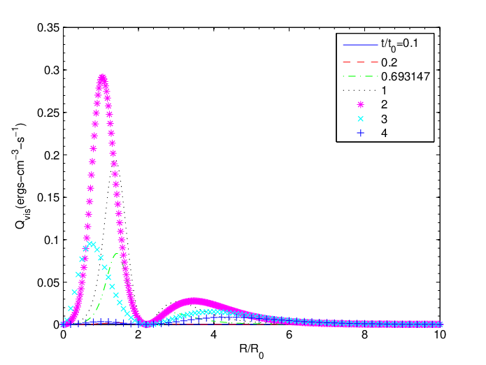
Figure 3 shows , and , and a panel showing their volume integrals together with the magnetic energy, which is the volume integral of . The plots of the heating rates suggest that different heating and cooling processes are important at different times during the acceleration process. Mainly for , and some intervals in the range , , but otherwise tends to significantly dominate . The plots of the volume integrated Joule and viscous heating rates show that Joule heating dominates viscous heating for , but not by much. Overall, compressive heating and cooling dominate the heating effect of and . is relatively large and positive for , and negative and relatively large in magnitude at later times, suggesting a strong cooling effect due to rarefaction . Characteristic mean chromospheric heating rates, assuming emission over a height range km, are ergs-cm-2-s-1/ km = ergs-cm-3-s-1 (Withbroe & Noyes 1977; Vernazza, Avrett & Loeser 1981; Anderson & Athay 1989). Then, locally and for tens of seconds, the estimated values of , and especially the magnitude of are comparable to, or far exceed the mean chromospheric heating rate.
Determining , and as in §6.1.1 gives ergs. About of the magnetic energy of ergs that is expended in accelerating the plasma, and heating it by resistive dissipation is converted into bulk flow kinetic energy. The value of is of the same order of magnitude as the larger values of the magnetic energy in Fig. 3. This is consistent with the fact that the magnetic field provides the energy for the acceleration and heating process. About 98% of is due to Pedersen current dissipation. Viscous heating exceeds Joule heating by a factor . The net compressive heating rate is relatively large and negative, indicating a net cooling effect during the acceleration process.
The energy estimates presented here are crude because they are not constrained by an energy equation. The question of the degree to which these estimates are realistic can be addressed in a meaningful way only by using models that include an energy equation. That equation couples , and to one another, and to radiative cooling, and diffusive and convective thermal energy flow. Solving an energy equation self-consistently as part of the model is also the only way to obtain a meaningful estimate of the variation of in space and time.
6.1.3. Energy and Mass Fluxes into the Corona
Ji et al. (2012) report observations of impulsive coronal heating associated with upward mass flows originating in photospheric regions of strong magnetic field in intergranular lanes. The flows from the photosphere into the corona are observed to occur along magnetic loops with diameters km, comparable to the reported diameters of type 2 spicules. Some of these flows are observed as RBE’s. The observations of Ji et al. are consistent with the suggestion that type 2 spicules are an important source of mass and energy for the corona. Semi-empirical analyses of De Pontieu et al. (2011) and Klimchuk (2012) respectively support and refute the possibility that type 2 spicules make a significant contribution of mass and energy to the corona.
The question of how much energy and mass type 2 spicules contribute to the corona is addressed here by computing the horizontal area and time averaged vertical mass flux, and electromagnetic, convective thermal, and bulk kinetic energy fluxes for the solutions presented here. These fluxes are evaluated at the height above the reference height at which the density is cm-3, defined here as the top of the chromosphere. They are upper limits to the mass and energy fluxes into the corona.
Let km, and . The average mass flux over the area , and time interval is
| (26) |
The average convective thermal energy flux .
The average bulk kinetic energy flux is
| (27) |
The average electromagnetic energy flux is computed using the component of the Poynting flux. Equations (17) and (23) are used to compute and . Then
| (28) |
Given the estimated total energy flux into the corona due to a single spicule, and assuming the spicules occur with a frequency such that they balance a coronal energy loss flux over the entire surface area of the Sun, the type 2 spicule occurrence frequency for a given solution is estimated as
| (29) |
Here is expressed in number per 100 s because this is a characteristic observed spicule lifetime. Choose ergs-cm-2-s-1.
For the solution in §6.1.2, , and . A characteristic solar wind mass flux at the base of the corona is g-cm-2-s-1 (Withbroe & Noyes 1977). Then dominates the energy flux, and is comparable to the average coronal energy loss during a time . The value of implies that if all of contributes to balancing coronal energy loss, then essentially all the spicule mass injected into the corona must return to the chromosphere, but this mass must be in the corona long enough to transfer all of its energy to coronal plasma. The value of is times larger than that inferred from the semi-empirical estimate of Judge & Carlsson (2010) that there are type 2 spicules distributed over the surface of the Sun at any given time.
The value ergs-cm-2-s-1 used above is a characteristic value for the coronal energy loss. The value of this loss varies over the surface of the Sun. Withbroe & Noyes (1977) give values of ergs-cm-2-s-1 for quiet Sun, coronal hole, and active regions. Using these values in Eq. (29) gives values for , and 82 times larger than the value inferred from Judge & Carlsson (2010). Given observational and model uncertainties, this suggests type 2 spicules may make a significant contribution to coronal energy input in quiet Sun regions, possibly also in coronal holes, but not in active regions.
6.2. Solution 2
For this solution G and km. Then G. The increase in by a factor of 2 requires that be reduced by a factor of 4 to keep . For the BG state and . Plots for Solution 2 are not included because they are similar in shape to those for Solution 1. The flow is localized within a diameter km. The maximum of is 77.5 km-s-1. If , the maximum of is 397.2 km-s-1. The maximum values of , and during the main phase of the acceleration are roughly 4, 30-40, 10, and 4-5 times their values for Solution 1.
Here ergs. Then of the magnetic energy of ergs that is expended in accelerating the plasma and heating it by resistive dissipation is converted into bulk flow kinetic energy. About 97% of is due to Pedersen current dissipation. The total thermal energy generated by Joule and viscous dissipation is greater than the net cooling due to rarefaction.
The estimated mass and energy fluxes into the corona are , and for ergs-cm-2-s-1. The energy injected into the corona is times less than for Solution 1, and the required value of is correspondingly times larger. The larger contribution of Solution 1 to the coronal energy input is due to the larger diameter of the region where the acceleration and heating are concentrated. An important unknown quantity is the occurrence frequency of spicules as a function of their diameter and energy content.
7. Conclusions
The HI viscous force can have a strong braking effect on type 2 spicule acceleration if it is driven by Lorentz forces associated with current densities localized within diameters km, corresponding to for the values of used here. If the actual characteristic radii within which the current density is localized are much larger, then the effect of viscous braking is expected to be significantly smaller. This follows from a dimensionless form of the momentum Eq. (3), which shows that the Lorentz force is , while the viscous force is , where is a Reynold’s number, and is a characteristic density. Then if all other input parameters are held constant, the ratio of the Lorentz force to the viscous force is .
The maximum vertical speeds of and 77 km-s-1 for the solutions presented here are at the lower end of type 2 spicule speeds. Significantly higher speeds might be possible in models not restricted to using values of sufficiently small so the effects of in the momentum equation can be neglected.
Joule and compressive heating dominate during the early stage of acceleration. Viscous heating dominates at later times when velocity gradients are largest, but the cooling rate due to rarefaction, corresponding to , more than cancels this heating rate. The total thermal energy generated by viscous dissipation during the acceleration process is an order of magnitude larger than that due to Joule dissipation, but the total cooling due to rarefaction can be comparable to or larger in magnitude than this energy. These are crude estimates since the model does not include an energy equation.
If all the upward spicule energy flux in the upper chromosphere contributes to coronal energy input, the energy injected by type 2 spicules into the corona may provide a significant fraction of the coronal energy input in quiet regions, possibly also in coronal holes, but not in active regions.
Magnetic flux emergence through the photosphere in inter-granular lanes is a likely source of non-force free current systems that accelerate type 2 spicules through the associated Lorentz force. This conclusion is based on the following complementary sets of observations, and on the MHD simulations cited in §2.2. (1) Type 2 spicules are localized on scales km perpendicular to their direction, consistent with inter-granular lane spatial scales. (2) Magnetic flux continually emerges through the photosphere in inter-granular lanes, with quiet Sun field strengths up to several hundred Gauss in internetwork, G in network, and with the emergence first appearing as a region of mixed polarity, nearly horizontal flux (Lites et al. 1996; Orozco Suárez et al. 2007; Lites et al. 2008; Lites 2009). The emerging magnetic structures become more vertical and quasi-cylindrical as they rise, similar to the geometry of type 2 spicules. (3) On the orders of magnitude larger scales of emerging sunspots, pores, and active regions, emerges carrying currents generated below the photosphere (Leka et al. 1996; Lites et al. 1998; Burnette et al. 2004; Sun et al. 2012). Flaring phenomena in these regions include acceleration of plasma up to speeds times greater than those of type 2 spicules. The field emerges as mixed polarity, nearly horizontal flux ropes with bipolar geometries, and field strengths G. The topology becomes more complex as the field rises into the chromosphere. Lites et al. (1998) emphasize that sections of these flux ropes can attain kilo-Gauss strength after they become nearly vertical as they flow out of the flux emergence region and rise into the chromosphere. This vertical, quasi-cylindrical geometry is similar to type 2 spicule geometry on smaller scales. By analogy, the observations of flux emergence with plasma acceleration on these relatively larger, better resolved scales support the proposition that emerging non-potential inter-granular flux is a source of current systems that drive type 2 spicules. At present there do not appear to be any other type 2 spicule acceleration mechanisms that are as strongly supported by observations.
The chromosphere is a highly resistive medium with respect to the Pedersen current density ( in the chromosphere) due to the combination of weak ionization and strong magnetization, which distinguishes the chromosphere from the weakly ionized, weakly magnetized photosphere, and the strongly ionized, strongly magnetized corona (Goodman 2000, 2004). Here “highly resistive” means the Pedersen resistivity is orders of magnitude larger than . This raises the following questions: (1) If emerging magnetic flux is considered as a driver of type 2 spicules, are the associated currents strong enough to cause type 2 spicule acceleration? (2) If the answer is yes, is the associated with emerging flux sufficiently dissipated by Pedersen current dissipation below the height at which spicules form so that the Lorentz force cannot be a major component of the force that accelerates type 2 spicules? At present these questions cannot be answered for the following reasons: (1) The formation heights of type 2 spicules are not known, other than that they form somewhere in the chromosphere. (2) An approximate, meaningful answer to these questions can be obtained from simulations of instances of the flux emergence process that include the essential physics, and use spatial and temporal resolutions sufficient to accurately compute , and the associated Lorentz force and . Such simulations do not yet exist. The 3D simulations of flux emergence by Arber et al. (2007) are a step towards developing such a simulation, and suggest that as flux rises into the chromosphere, there is strong dissipation of , consistent with general results in Goodman (2000, 2004), and the expectation that the atmosphere becomes increasingly force free with increasing height.
References
- [1] Anderson, L.S. & Athay, R.G. 1989, ApJ, 346, 1010
- [2] Arber, T.D., Haynes, M. & Leake, J.E. 2007, ApJ 666, 541
- [3] Burnette, A.B., Canfield, R.C. & Pevtsov, A.A. 2004, ApJ, 606, 565
- [4] Centeno, R., Trujillo Bueno, J. & Andrés Asensio Ramos, A. 2010, ApJ, 708, 1579
- [5] De Pontieu, B., Hansteen, V. H., Rouppe van der Voort, L., van Noort, M., & Carlsson, M. 2007 a, ApJ, 655, 624
- [6] De Pontieu, B., McIntosh, S. W., Carlsson, M., et al. 2007 b, Science, 318, 1574
- [7] De Pontieu, B., McIntosh, S., Hansteen, V. H., et al. 2007 c, PASJ, 59, 655
- [8] De Pontieu, B., McIntosh, S.W., Carlsson, M., Hansteen, V.H., Tarbell, T.H., Boerner, P., Martinez-Sykora, J., Schrijver, C.J. & Title, A.M. 2011, Science, 331, 55
- [9] De Pontieu, B., Carlsson, M., Rouppe van der Voort, L.H.M., Rutten, R.J., Hansteen, V.H. & Watanabe, H. 2012, ApJ, 752, L12
- [10] De Wijn, A. 2012 ApJ, 757, L17
- [11] De Wijn, A.G., Stenflo, J.O., Solanki, S.K. & Tsuneta, S. 2009, Space Sci. Rev., 144, 275
- [12] Goodman, M.L. 2000, ApJ, 533, 501
- [13] Goodman, M.L. 2004, A&A, 416, 1159
- [14] Goodman, M.L. 2012, ApJ, 757, 188
- [15] Goodman, M. L. & Judge, P.G. 2012 , ApJ, 751, 75
- [16] Ji, H., Cao, W. & Goode, P.R. 2012, ApJ, 750, L25
- [17] Judge, P. G. & Carlsson, M. 2010, ApJ, 719, 469
- [18] Klimchuk, J.A. 2012, J. Geophys. Res., 117, A12102, doi:10.1029/2012JA018170
- [19] Langangen, Ø., De Pontieu, B., Carlsson, M., et al. 2008, ApJ, 679, L167
- [20] Leka, K.D., Canfield, R.C., McClymont, A.N. & van Driel-Gesztelyi, L. 1996, ApJ, 462, 547
- [21] Lites, B.W. 2009, Space Sci. Rev., 144, 197
- [22] Lites, B.W., Kubo, M., Socas-Navarro, H., Berger, T., Frank, Z., Shine, R., Tarbell, T., Title, A., Ichimoto, K., Katsukawa, Y., Tsuneta, S. & Suematsu,Y. 2008, ApJ, 672, 1237
- [23] Lites, B.W., Leka, K.D., Skumanich, A., Martínez Pillet, V. & Shimizu, T. 1996, ApJ, 460, 1019
- [24] Lites, B.W., Skumanich, A. & Martínez Pillet, V. 1998, A&A, 333, 1053
- [25] López Ariste, A. & Casini, R. 2005, A&A, 436, 325
- [26] Martínez-Sykora, J., Hansteen, V. & Carlsson, M. 2009, ApJ, 702, 129
- [27] Martínez-Sykora, J., Hansteen, V. & Moreno-Insertis, F. 2011 ApJ, 736, 9
- [28] McIntosh, S. W. & De Pontieu, B. 2009, ApJ, 706, L80
- [29] Mitchner, M. & Kruger, C.H. 1973, Partially Ionized Gases (Wiley, New York)
- [30] Mihalas, D. & Mihalas, B.W. 1984, Foundations of Radiation Hydrodynamics (Oxford Univ. Press, New York)
- [31] Orozco Suárez, D., Bellot Rubio, L.R., del Toro Iniesta, J.C., Tsuneta, S., Lites, B.W., Ichimoto, K., Katsukawa, Y., Nagata, S., Shimizu, T., Shine, R.A., Suematsu, Y., Tarbell, T.D. & Title, A.M. 2007, ApJ, 670, L61
- [32] Osterbrock, D.E. 1961, ApJ, 134, 347
- [33] Pereira, T.M.D., De Pontieu, B. & Carlsson, M. 2012, ApJ, 759, 18
- [34] Ramelli, R., Bianda, M., Merenda, L., & Trujillo Bueno, J. 2006, in ASP Conf. Ser 358, Solar Polarization 4, ed. R. Casini & B. Lites (San Francisco, CA: ASP), 448
- [35] Rouppe van der Voort, L., Leenaarts, J., De Pontieu, B., Carlsson, M., & Vissers, G. 2009, ApJ, 705, 272
- [36] Sánchez Almeida, J. & Martínez González, M. 2011, Solar Polarization 6. Proceedings of a conference held in Maui, Hawaii, USA on May 30 to June 4, 2010. Edited by J. R. Kuhn, D. M. Harrington, H. Lin, S. V. Berdyugina, J. Trujillo-Bueno, S. L. Keil, and T. Rimmele. San Francisco: Astronomical Society of the Pacific, 2011., p.451.
- [37] Sekse, D. H., Rouppe van der Voort, L. & De Pontieu, B. 2012, ApJ, 752, 108
- [38] Stenflo, J.O. 2012, A&A, 541, A17
- [39] Stenflo, J.O. 2013, A&A Rev., 21, 66S
- [40] Sun, X., Hoeksema, J. Todd, Liu, Y., Wiegelmann, T., Hayashi, K., Chen, Q. & Thalmann, J. 2012, ApJ748, 77
- [41] Tavabi, E., Koutchmy, S., & Ajabshirizadeh, A. 2011, New Astronomy, 16, 296
- [42] Thompson, Philip A. 1988, Compressible Fluid Dynamics (McGraw-Hill Inc., Advanced Engineering Series)
- [43] Trujillo Bueno, J. 2005, in The Dynamic Sun: Challenges for Theory and Observations, ed. D. Danesy et al. (Published on CDROM, p. 7.1; ESA SP-600; Noordwijk: ESA)
- [44] Tsiropoula, G., Tziotziou, K., Kontogiannis, I., Madjarska, M.S., Doyle, J.G. & Suematsu, Y. 2012, Space Sci. Rev., 169,181
- [45] van Noort, M.J. & Rouppe van der Voort, L.H.M. 2006, ApJ, 648, L67
- [46] Vernazza, J. E., Avrett, E. H. & Loeser, R. 1981, ApJS, 45, 635
- [47] Withbroe, G.L. & Noyes, R.W. 1977, ARA&A, 15, 363