Optimal Resource Allocation in Full-Duplex Wireless-Powered Communication Network
Abstract
This paper studies optimal resource allocation in the wireless-powered communication network (WPCN), where one hybrid access-point (H-AP) operating in full-duplex (FD) broadcasts wireless energy to a set of distributed users in the downlink (DL) and at the same time receives independent information from the users via time-division-multiple-access (TDMA) in the uplink (UL). We design an efficient protocol to support simultaneous wireless energy transfer (WET) in the DL and wireless information transmission (WIT) in the UL for the proposed FD-WPCN. We jointly optimize the time allocations to the H-AP for DL WET and different users for UL WIT as well as the transmit power allocations over time at the H-AP to maximize the users’ weighted sum-rate of UL information transmission with harvested energy. We consider both the cases with perfect and imperfect self-interference cancellation (SIC) at the H-AP, for which we obtain optimal and suboptimal time and power allocation solutions, respectively. Furthermore, we consider the half-duplex (HD) WPCN as a baseline scheme and derive its optimal resource allocation solution. Simulation results show that the FD-WPCN outperforms HD-WPCN when effective SIC can be implemented and more stringent peak power constraint is applied at the H-AP.
Index Terms:
Wireless-powered communication network (WPCN), wireless energy transfer (WET), full-duplex (FD) system, resource allocation, convex optimization.I Introduction
Traditionally, fixed energy sources (e.g. batteries) have been used to power energy-constrained wireless networks, such as sensor networks, which lead to limited operation time. Although the lifetime of wireless networks can be extended by replacing or recharging the batteries, it may be inconvenient, costly, and even dangerous (e.g., in a toxic environment) or infeasible (e.g., for sensors implanted in human bodies). As an alternative solution, energy harvesting (see e.g., [1], [2] and the references therein) has recently received a great deal of attention since it provides more cost-effective and truly perpetual energy supplies to wireless networks through scavenging energy from the environment.
Among other commonly used energy sources (e.g. solar and wind), radio signal radiated by ambient transmitters becomes a viable new source for energy harvesting. In particular, harvesting energy from the far-field radio-frequency (RF) signal transmission opens a new avenue for the unified study of wireless power transmission and wireless communication since radio signals carry energy and information at the same time. There are two main paradigms of research along this direction. One line of work focuses on studying the so-called simultaneous wireless information and power transfer (SWIPT) by characterizing the achievable trade-offs in simultaneous wireless energy transfer (WET) and wireless information transmission (WIT) with the same transmitted signal. SWIPT has recently been investigated for various channel setups, e.g., the point-to-point additive white Gaussian noise (AWGN) channel [3], [4], the fading AWGN channel [5], [6] the multi-antenna channel [7]-[9], the relay channel [10], [11], and the multi-carrier based broadcast channel [12]-[14].
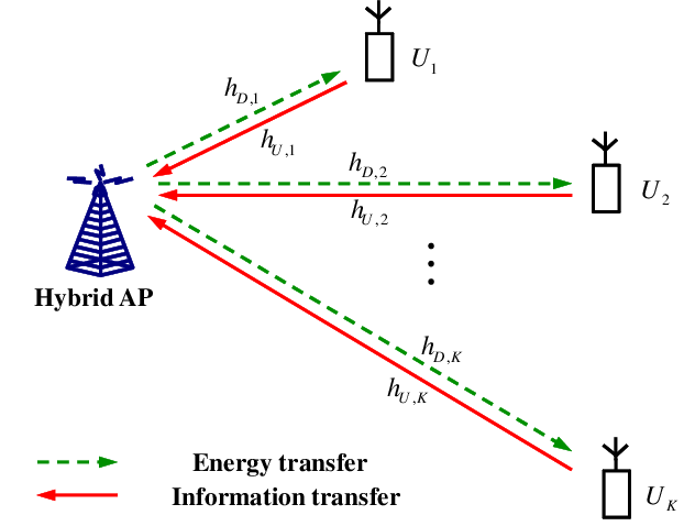
Another line of research is aimed to design a new type of wireless network termed wireless-powered communication network (WPCN) in which wireless terminals communicate using the energy harvested from wireless power transmissions. The WPCN has been studied under various network setups, such as cellular network [15], random-access network [16], and multi-hop network [17]. In [18] and [19], another type of WPCN was investigated, where mobile charging vehicles are employed to wirelessly power the user devices in the network. In addition, the wireless-powered cognitive radio network was considered in [20], where active primary users are utilized as energy transmitters for charging their nearby secondary users. Furthermore, in our previous work [21] we have studied one particular WPCN model, as shown in Fig. 1, where a hybrid access-point (H-AP) operating in time-division half-duplex (HD) mode coordinates WET/WIT to/from a set of distributed users in the downlink (DL) and uplink (UL) transmissions, respectively. It has been shown in [21] that there exists a fundamental trade-off in allocating DL time for WET and UL time for WIT in the HD WPCN, since increasing DL time increases the amount of harvested energy and hence the UL transmit power at each user, but also decreases users’ UL time for WIT given a total DL and UL time constraint.
On the other hand, there has been recently a growing interest in full duplex (FD) based wireless systems, where the wireless node transmits and receives simultaneously in the same frequency band, thus potentially doubling the spectral efficiency. However, due to the simultaneous transmission and reception at the same node, FD systems suffer from the self-interference (SI) that is part of the transmitted signal of a FD node received by itself, thus interfering with the desired signal received at the same time. Self-interference cancellation (SIC) is a key challenge for implementing FD communication since the power of SI typically overwhelms that of the desired signal. Various SIC techniques have been proposed in the literature (see e.g., [22]-[25] and the references therein), which are generally based on either analog-domain SIC (i.e., SIC in the wireless propagation channel or before the received signal is processed by analog-to-digital conversion (ADC)), digital-domain SIC (i.e., SIC after ADC by digital signal processing techniques), or their assorted combinations. By state-of-the-art SIC techniques today, it has been reported that SIC up to dB higher power of the desired signal can be implemented [25]. In addition, various effects of practical hardware limitations on FD communications, e.g., the finite dynamic range of transmit and/or receive filters [26], [27], have been investigated. Furthermore, full-duplex techniques have been applied in various wireless communication applications for performance enhancement, e.g., spectral efficiency in relay network [28], multi-user cellular network [29], wireless physical layer security [30], and cognitive radio network [31].
In this paper, we apply the FD technique to the WPCN shown in Fig. 1, to further improve throughput. We assume that the H-AP operates in the FD mode to broadcast energy and receive information to/from the distributed users simultaneously over a given frequency band, thus significantly saving the time for separate DL WET and UL WIT as compared to the HD-WPCN considered in [21]. The proposed WPCN with the H-AP operating in FD mode is thus termed full-duplex WPCN (FD-WPCN), to differ from its HD-WPCN counterpart in [21]. It is worth noting that the FD technique applied at the H-AP in our proposed FD-WPCN is for hybrid energy/communication transmission/reception, which is in sharp contrast to conventional setups with FD communications. However, similar to FD communication systems, the proposed hybrid energy/communication FD system is also subject to the practical issue of imperfect SIC at the H-AP, i.e., the interference due to the DL energy signal is not perfectly cancelled at the receiver for decoding the UL information.
The main results of this paper are summarized as follows:
- •
For the proposed FD-WPCN, we present a new protocol to enable simultaneous WET in the DL and WIT in the UL over the same band. It is assumed that the H-AP operates in FD mode, while the users all operate in time division HD mode for the ease of implementation, which transmit independent information to the H-AP by time-division-multiple-access (TDMA) in the UL and harvest energy in the DL when they do not transmit. We also compare the proposed protocol for FD-WPCN with the harvest-then-transmit protocol proposed in [21] for HD-WPCN.
- •
Under the proposed protocol for FD-WPCN, we characterize the maximum weighted sum-rate (WSR) of users in FD-WPCN, by jointly optimizing the time allocated to the H-AP for DL WET and users for UL WIT and the transmit power of the H-AP over time subject to a given total time constraint as well as the average and peak transmit power constraints at the H-AP. For the purpose of exposition, we first consider the ideal case of perfect SIC at the H-AP in FD-WPCN. It is shown that the WSR maximization problem in this case is convex, and hence we obtain the closed-form solution for the optimal time and power allocations by applying convex optimization techniques. It is revealed that the optimal time and power allocation is aligned with maximally exploiting the opportunistic communication gain in the network, i.e., more time is assigned to the users with stronger channels and/or higher rate weights (priorities) in UL WIT, while more power is broadcast by the H-AP in DL WET over time slots of the users with weaker channels and/or lower weights.
- •
We then study the practical case with imperfect SIC in FD-WPCN. In this case, the WSR maximization problem is shown to be non-convex, and thus is difficult to be solved optimally. Alternatively, we propose an efficient algorithm to find at least one locally optimal solution for this problem based on the optimal solution obtained for the ideal case without SI by iteratively optimizing the time and power allocations to maximize the WSR.
- •
Furthermore, we investigate the WSR maximization problem in a baseline HD-WPCN system based on the harvest-then-transmit protocol proposed in [21]. It is worth pointing out the main difference between the optimization problems considered in this work and our prior work [21] for HD-WPCN. In this paper, we study the joint power and time allocations subject to both the average and peak transmit power constraints in HD-WPCN, whereas only time allocation is considered in [21] by assuming constant transmit power at the H-AP. By comparing the achievable rates of FD- versus HD-WPCNs, it is revealed that the former is more beneficial than the latter when the SI can be more effectively cancelled at the H-AP and/or the peak transmit power constraint at the H-AP is more stringent.
The rest of this paper is organized as follows. Section II introduces the FD-WPCN model and the proposed transmission protocol. Section III presents the optimal time and power allocation solutions to the WSR maximization problems in FD-WPCN for both the ideal case of perfect SIC and the practical case with imperfect SIC, respectively. Section IV addresses HD-WPCN, and shows the optimal solution for WSR maximization in this case. Section V presents simulation results for comparing the performance of FD-WPCN against HD-WPCN. Finally, Section VI concludes the paper.
II System Model
As shown in Fig. 1, this paper considers a WPCN with WET in the DL and WIT in the UL. The network consists of one H-AP and users (e.g., sensors) denoted by , , operating over the same frequency band. It is assumed that users are sufficiently separated from each other. The H-AP is equipped with two antennas, and each user terminal is equipped with one antenna. The H-AP is assumed to have a stable energy supply, whereas each user terminal does not have any embedded energy sources. As a result, the users need to replenish energy from the received signal from the H-AP in the DL, which is then used to power operating circuit and transmit information in the UL. In this paper, we focus on the case of FD-WPCN where the H-AP operates in FD mode to broadcast energy for the DL WET and receive information for the UL WIT at the same time, while the users are assumed to all operate in time-division HD mode to harvest energy in the DL and transmit information in the UL orthogonally over time, for the ease of implementation. For the purpose of comparison, we also consider the case of HD-WPCN where the H-AP also operates in time-division HD mode, as studied in our previous work [21].
II-A FD-WPCN
In FD-WPCN, the H-AP operates in FD mode by utilizing one antenna for transmitting energy to users in DL and the other antenna for receiving information from users in UL simultaneously over the same bandwidth. The DL channel from the H-AP to and the corresponding reversed UL channel are denoted by complex coefficients and , , respectively. In addition, there exists a loopback channel at the H-AP, through which the transmitted DL energy signal of one antenna is received at the other antenna in addition to the UL information signal received from users. It is assumed that at the H-AP, analog domain SIC [22], [23] is first performed,11 1 We refer to SIC before A/D conversion as analog domain SIC, by e.g., offsetting the two transmit antennas by half a wavelength [22], or using an extra transmit RF chain to generate a reference RF signal [23], while SIC after A/D conversion, commonly referred to as digital domain SIC, will be considered later. thus denotes the effective loopback channel after analog domain SIC at the H-AP. We also assume that , , , and all follow quasi-static flat-fading, and the channels remain constant during each block transmission time, denoted by , for the system of interest. It is further assumed that the H-AP knows perfectly and , .

In FD-WPCN, simultaneous WET in DL and WIT in UL can be achieved, as shown in Fig. 2. Each transmit block is divided into slots each with duration of , . The th slot is a dedicated power slot for DL WET only22 2 This is to ensure that even for the case with one user in the system, i.e., , the user can still receive energy from the dedicated power slot. and the th slot, , is used for both DL WET and UL WIT. During the th slot, the H-AP broadcasts wireless energy with transmit power, denoted by , to all users in the network. We thus have
| (1) |
In addition, the average transmit power of the H-AP over slots in each block and the peak transmit power of the H-AP at each slot are denoted by and , respectively, i.e.,
| (2) |
| (3) |
In UL, we assume that the users transmit independent information to the H-AP using TDMA, i.e., the th slot is allocated to user for WIT, . Specifically, during the th slot in each block, the H-AP broadcasts energy using one antenna and receives information from using the other antenna simultaneously, since the H-AP operates in FD mode. On the other hand, each user , , transmits its own information to the H-AP in the th slot, but cannot receive energy from the H-AP in the same slot, since it operates in time-division HD mode and has one single antenna. Instead, harvests energy from the H-AP during the other slots during which it is not scheduled for information transmission, and stores the energy harvested to be used in future.
Consider the th slot in one block of interest, , during which the transmitted signal of the H-AP is denoted by .33 3 Note that ’s can also be used to send DL information (e.g., control signals from the H-AP to users) at the same time, which is not considered further in this paper. Interested readers may refer to the literature on SWIPT [5]-[14]. We assume that is a pseudo-random sequence which is a prior known at the H-AP44 4 This facilities the implementation of SIC at the H-AP, as will be shown next. satisfying . During the th slot, the received signal at , , is then expressed as
| (4) |
where and denote the received signal and noise at , respectively. It is assumed that is sufficiently large such that the energy harvested due to the receiver noise is negligible. Furthermore, energy harvested due to the received UL WIT signals from other users is also assumed to be negligible since users are sufficiently separated from each other and their transmit power level is much lower as compared to in practice. Thus, the amount of energy harvested by during the th slot can be expressed as
| (5) |
where , , is the energy harvesting efficiency at . For convenience, we assume in the sequel of this paper without loss of generality. From (5), the average harvested energy of in each block is thus expressed as
| (6) |
On the other hand, during the th slot with , transmits its own information to the H-AP using a fixed portion of its average harvested energy per block given by (6). Within amount of time allocated to for UL WIT in slot , the average transmit power of is thus given by
| (7) |
where denotes the portion of the average harvested energy used for WIT by in steady state. In this paper, we assume that ’s are given constants. We further denote as the signal transmitted by during slot . For each user, is assumed to be of zero mean and unit power, i.e., and . The received signal at the H-AP in the th slot is then expressed as
| (8) |
where , , and denote the received signal, the SI due to simultaneously transmitted energy signal , and the noise at the H-AP, respectively. It is assumed that , , where stands for a circularly symmetric complex Gaussian (CSCG) random variable with mean and variance .
Without loss of generality, the effective loopback channel after analog domain SIC, , can be expressed as
| (9) |
where and , respectively, denote the power and normalized complex coefficient of the loopback channel after analog domain SIC, with . Even after analog domain SIC, however, the power of remaining SI can be still much larger than that of received signal in practice [27], i.e., . This raises in the following considerations. First, the received signal at the H-AP given by (8) is distorted due to limited transmitter and receiver dynamic ranges due to large power of SI, which introduces additional noise whose power is proportional to transmit and/or receive power at the H-AP (see e.g., [26] and [27]). For the purpose of exposition, we assume the same signal processing implemented at the H-AP as in [27] with ideal automatic gain control (AGC) and infinite transmitter dynamic range. Thus, the additional receiver noise, denoted by , is merely due to finite receiver dynamic range and the resulting quantization error after ADC [27], where with and is derived from (8) as
| (10) |
Furthermore, although channel estimation can be made sufficiently accurate such that performance degradation due to the estimation errors in and , , is assumed to be negligible, performance degradation due to estimation error of cannot be neglected in general due to more dominant power of SI than that of received information signal at the H-AP. We thus denote with and denoting the estimation of and channel estimation error, respectively. It is assumed that and . Given , we can apply digital domain SIC by subtracting known SI as in [26], i.e., from the received signal after ADC. After ADC and digital domain SIC, the received signal can be expressed as
| (11) |
It is worth noting that in (10) since the power of SI is in general much larger than those of received information signal from and receiver noise, based on which the received signal-to-interference-plus-noise ratio (SINR) of after ADC and digital domain SIC can be expressed from (11) as
| (12) |
where , , and denotes the power of effective SI at the th slot with
| (13) |
From (12), the achievable rate of for the case of FD-WPCN in bits/second/Hz (bps/Hz) can be expressed as
| (14) |
where , , and represents the SINR gap from the additive white Gaussian noise (AWGN) channel capacity due to the practical modulation and coding scheme (MCS) used. In (14), represents the residual SI power55 5 Here, the residual SI includes the quantization noise whose power is also proportional to . due to finite receiver dynamic range and imperfect channel estimation. Furthermore, it is worth noting that switching transmit and receive antennas at the H-AP does not change the achievable rate in (14) since depends only on , which is the product of the UL and DL channel power gains.
II-B HD-WPCN

In the case of HD-WPCN, we assume that the harvest-then-transmit protocol proposed in [21] is employed to achieve orthogonal WET in DL and WIT of users in UL, as shown in Fig. 3. Since neither H-AP nor users can transmit and receive signals at the same time, with the harvest-then-transmit protocol, energy is broadcast in DL during the th slot only whereas the th slot, , is used for UL WIT only, in which users transmit their independent information to the H-AP by TDMA. It then follows that
| (15) |
Denote as the transmit power of the H-AP for DL WET in slot in the case of HD-WPCN. The achievable rate of for UL WIT in bps/Hz is then given by [21]
| (16) |
where . Like the case of FD-WPCN, we have and as the average and peak transmit power constraints at the H-AP, respectively; thus we have .
III Optimal Time and Power Allocation in FD-WPCN
In this section, we study the joint time and power allocation in FD-WPCN to maximize the throughput. Specifically, from (14), we aim to maximize the WSR of all users in UL WIT, which is formulated as the following optimization problem.
Note that is the given non-negative rate weight for . Let . By changing the values of ’s in (P1), we are able to characterize the maximum throughput of FD-WPCN with different rate trade-offs among the users. In the following, we first investigate time and power allocations to maximize the WSR in (P1) for an ideal FD-WPCN assuming perfect SIC, i.e., in (14), and then study the general case with finite SI, i.e., .
III-A FD-WPCN with Perfect SIC
Without SI, the achievable rate of user in the -user FD-WPCN is modified from (14) as
| (17) |
Even with each user’s achievable rate given by (17) assuming perfect SIC, problem (P1) is still non-convex due to the non-convexity shown in the average power constraint given by (2). Similarly as in [14] and [32], we change the variables as , , to make this problem more analytically tractable, where denotes the energy broadcast by the H-AP during the th slot. From (17), the achievable rate of can then be expressed as
| (18) |
where and . Accordingly, problem (P1) in the case of perfect SIC can be reformulated as
| (19) |
| (20) |
where (19) and (20) correspond to the original constraints in (2) and (3), respectively. By introducing new variables in , joint time and power allocation in problem (P1) is converted to joint time and energy allocation in problem (P2).
It is worth noting that for any given , the objective function of problem (P2) is a monotonically increasing function of each individual , , and thus the constraint in (19) should hold with equality at the optimal energy allocation (otherwise, the objective function can be further increased by increasing some ’s). Therefore, the optimal time and energy allocation solution for (P2) can be equivalently obtained by solving the following problem:
| (21) |
| (22) |
| (23) |
| (24) |
with given by
| (25) |
Lemma 3.1: is a jointly concave function of and , .
Proof.
Please refer to Appendix A. ∎
From Lemma 3.1, it follows that the objective function of (P3) is jointly concave over and . Therefore, problem (P3) is a convex optimization problem together with the facts that the average power constraints in (2) of (P1), which is non-convex, is now transformed to a sum-energy constraint in (22) of (P3), which is affine, and furthermore the constraint in (23) is an affine function of both and . Problem can thus be solved by Lagrangian duality, shown as follows.
From (21), (22), and (25), Lagrangian of is given by
| (26) |
with and denoting the Lagrange multipliers associated with the constraints in (21) and (22), respectively. The dual function of problem (P3) is then given by
| (27) |
where is a feasible set of specified by (23) and (24). The dual problem of (P3) is thus given by .
Proposition 3.1: Given , , and strictly positive weights , , the maximizer of in (26) is given by and , where
| (28) |
| (29) |
| (30) |
| (31) |
with , and denoting the solution of where
| (32) |
Proof.
Please refer to Appendix B. ∎
According to Proposition 3.1, and under which in (27) is achived can be attained as follows. We first obtain and by iteratively optimizing between and using (30) and (31), respectively, with one of them being fixed at one time until they both converge. We then compute and using (28) and (29), respectively. With obtained for each given pair of and , the optimal dual variables and minimizing can then be efficiently found by sub-gradient based algorithms, e.g., the ellipsoid method [34], with the sub-gradient of given by , where
| (33) |
| (34) |
Denote the optimal time and energy allocation solution for , and equivalently for problem (P2), as and , respectively. It is then worth noting that the objective function of (P3) is a monotonically increasing function of each individual , for given , . Therefore, should hold at the optimal (otherwise, the objective function can be further increased by increasing some ’s). Furthermore, note that we obtain and at the optimal dual solution and . Therefore, we have , as well as to satisfy the constraint in (22). Once and for (P3) (or equivalently for (P2)) are obtained, the optimal power allocation solution for (P1) is obtained as , , in the case of perfect SIC. To summarize, one algorithm to solve (P1) is given in Table I.
| 1. Initialize and . 2. Repeat 1) Initialize and , . 2) Repeat i) Compute by (30). ii) Compute by (31). 3) Until and both converge. 4) Compute and by (28) and (29). 5) Compute the sub-gradient of by (33) and (34). 6) Update and using the ellipsoid method. 3. Until and converge to a predefined accuracy. 4. Set and , . 5. Obtain and . 6. Set , . |
The computation time of the algorithm given in Table I is analyzed as follows. The time complexities of steps 2.1)-2.3) is , while those of 2.4) and 2.5) are and , respectively. Note that only two dual variables, and , are updated by the ellipsoid algorithm regardless of the number of users, . The time complexity of step 2.6) is thus [34]. Therefore, the total time complexity of the algorithm in Table I is .
Next, to obtain more insight to the solution given in Proposition 3.1, we consider the special case of . From Proposition 3.1, and (or ) for problem (P2) when is given in the following corollary.
Corollary 3.1: For problem (P2) with , the optimal time and power allocation solutions are given by
| (35) |
where denotes the solution of with and is given by (32).
Proof.
Please refer to Appendix C. ∎
Corollary 3.1 indicates that given rate-weight vector , the maximum WSR of FD-WPCN without SI as is achieved by choosing only the th slot for DL WET, which has zero amount of time (i.e., ), and sending all available energy (cf. (19)) in this zero-time slot (i.e., , ). It is worth noting that in this case the WSR of the FD-WPCN is equivalent to that of the conventional -user TDMA network for UL WIT only, where each user is equipped with a constant energy supply to provide equal transmit energy consumption at each block denoted by and the UL channel for each user is given by , . It is also worth noting that in this special case, the FD-WPCN is in fact a HD-WPCN with and . When the sum-rate is maximized with , , it can be further shown that and , .
Note that when , should be strictly positive since ( if and if . Please see Appendix B for details.). It is thus shown from (29) that . It thus follows that if , then and thus , and vice versa if . For , results in as shown from (31), whereas does not necessarily imply as shown from (30). This is because , , represents the amount of energy that the H-AP broadcasts to ’s, , , during the th slot, while provided that , can transmit information to the H-AP even when the H-AP does not broadcast any energy during the slot, i.e., . Therefore, even when , it is possible to allocate zero transmit power to a slot with at the H-AP, i.e., . The only case where for given can yield is when the corresponding since should be zero for this case, according to (32).

It is also worth noting from Corollary 3.1 that in the case of , the algorithm given in Table I can be similarly applied to update and (or equivalently ) from any arbitrary point (,) toward given in (35). With , however, , , stops updating when it reaches , after which is updated such that . Fig. 4 shows and to maximize the sum-rate in a SI-free FD-WPCN with , , ,66 6 In Fig. 4, and are normalized for the convenience of illustration. In fact, this corresponds to the case with dBm in the practical simulation setup of Section V. Please refer to Section V for the detailed simulation setup. , and , . We consider two different values of maximum peak power, or . Furthermore, the DL and UL channels are assumed to be drawn from Rayleigh fading, i.e., and , , and sorted in an ascending order of in terms of , i.e., . For both cases with and , it is observed that no time and power is allocated to the th slot (dedicated power slot), i.e., , to maximize the sum-rate. When , it is observed that , i.e., the H-AP broadcasts energy in DL with power of during st-th slots in which the users with the weaker channel conditions transmit information in UL. Furthermore, of energy is broadcast from the H-AP during st-th slots, where . The remaining time is allocated to the slots in which the users with better channel conditions transmit information in UL, and with larger is allocated more time for UL WIT. In particular, it is also observed that , i.e., the H-AP does not broadcast energy in DL when the user with the best channel transmits information in UL in order to maximize the sum-rate. When , similarly, and the H-AP broadcasts of energy during the st-th slots where . In addition, and . From the above observations, it can be inferred that to maximize the WSR, the H-AP does not broadcast energy in DL when the users with larger ’s and/or ’s transmit information in UL, whereas it broadcasts energy only when the users with weaker channel conditions and/or smaller rate weights (priorities) transmit information.
Fig. 5 shows the achievable rate regions of a 2-user FD-WPCN with perfect SIC. It is assumed that , , , , and , . The channels between the H-AP and two users and are set such that and . We consider four different peak power values, , , , and . When , it is observed that the maximum achievable rate of is and the rate region of FD-WPCN in this case is equivalent to that of -user TDMA network for WIT only, which is obtained with (35). With finite , the achievable rate region is observed to be smaller as decreases.

III-B FD-WPCN with Finite SI
In the case of imperfect SIC with , problem (P1) is in general non-convex, and thus cannot be solved optimally in an efficient way. However, we can find one locally optimal solution for (P1) by setting for the case without SI from Proposition 3.1 as an initial point, and then updating and iteratively, shown as follows. Denote and as the time and power allocation obtained at the th iteration, respectively. We then have . At the -th iteration, we first update to obtain using . Then, is updated to obtain using and . The above iteration is repeated until the WSR cannot be further improved for problem (P1).
For simplifying the above updates, given by (14) is modified as
| (36) |
by assuming that the average power constraint in (2) holds with equality.77 7 The average power constraint in (2) may not hold with equality at the optimal time and power allocations in general for (P1), although this is usually desirable in practice since there is no energy wasted at the H-AP. We make this assumption here in order to have the rate function in (36) only dependent on and , but no more on other ’s and ’s, , as in (13). From (36), at the th iteration can be obtained as the solution of the following problem.
| (37) |
| (38) |
Lemma 3.2: Given , given in (36) is a concave function of , .
Proof.
Please refer to Appendix D. ∎
From Lemma 3.2, it follows that problem (P4) is convex. Therefore, problem (P4) can be solved by Lagrangian duality. From (36)-(38), the Lagrangian of (P4) is given by
| (39) |
where and denote the Lagrange multipliers associated with the constraints in (37) and (38), respectively. The dual function of problem (P4) is then given by , and the dual problem of (P4) is thus given by .
Proposition 3.2: Given , and where , the maximizer of is given by , where
| (40) |
where and is the solution of with defined as
| (41) |
Proof.
Please refer to Appendix E. ∎
It can be shown that is a monotonically increasing function of since . After obtaining with given and , the minimization of over and can be efficiently solved by the ellipsoid method [34], with the sub-gradient of , denoted as , given by
| (42) |
| (43) |
where , , are given by (40). The optimal solution of (P4), denoted by , is then obtained corresponding to the optimal dual solution of and after the ellipsoid method converges, and finally we have for given .
Once is obtained, at the th iteration can be attained using the obtained . Denote at the th iteration as , where . Since , , as shown in (40), we can thus take any value for such that . Furthermore, can be obtained by applying the gradient projection method based on (36), as follows:
| (44) |
| (45) |
where and are both small step sizes. In addition, denotes the gradient of with , , given by
| (46) |
Furthermore, denotes the feasible set of given and , defined by
| (47) |
Finally, in (44) denotes the operation of projection of onto . To summarize, one algorithm to solve problem (P1) with finite is given in Table II.
| 1. Initialize , obtained by solving (P1). 2. Repeat 1) Set . 2) Given , , and , solve (P4) by Proposition 3.2. 3) Update and using the ellipsoid method and sub-gradient of given by (42) and (43), and obtain . 4) Set . 5) Obtain using , , (36), and (44)-(47). 3. Until . |
At each iteration of the algorithm given in Table II, the computational complexity of step 2.2) is . Similarly to the case with perfect SIC in the previous subsection, computations are required for step 2.3). In step 2.5), , , and computations are required for computing in (46), in (44), and in (45), respectively. Therefore, the total time complexity of the algorithm in Table II is .
Remark 3.1: With , we can choose such that , resulting in , . In this special case, the FD-WPCN with finite SI is in fact equivalent to that in the previous ideal case of perfect SIC with .
IV Optimal Time and Power Allocation in HD-WPCN
In this section, we study the optimal time and power allocation in HD-WPCN to maximize the WSR. Given , from (16) the WSR maximization problem for HD-WPCN is formulated as
| (48) |
| (49) |
| (50) |
Problem (P4) is non-convex in general due to the non-concave objective function defined in (16) and non-convex average power constraint in (49). To solve problem (P4), we first consider the following WSR maximization problem for HD-WPCN when the transmit power of the H-AP is fixed as .
with defined in (18). As shown in [21], (P5) is convex and its optimal time allocation solution, denoted by , is given in the following lemma.
Lemma 4.1: For problem (P6), the optimal solution is given by
| (51) |
| (52) |
where , , is the solution of the following equations:
| (53) |
| (54) |
with being a constant under which .
Proof.
Please refer to [21]. ∎
With attained from Lemma 4.1, we can obtain the optimal power and time allocation solution for (P5), denoted by and , as given in the following proposition.
Proposition 4.1: The optimal transmit power solution for (P5) is . In addition, the optimal time allocation solution for (P5) is given by
| (55) |
| (56) |
where , , are given in (51) and (52), and , , and are solutions of the following equations:
| (57) |
| (58) |
Proof.
Please refer to Appendix F. ∎
From Proposition 4.1, it is observed that the optimal transmit power of the H-AP in HD-WPCN is always , regardless of the optimal time allocations. In addition, we can compute for (P5) efficiently as follows. First, we solve (P6) to obtain (one algorithm to solve (P6) is given in [21]). If , then the optimal time allocation solution for (P5) is , . Otherwise, if , then , and , , can be obtained from (56) via solving for ’s by a bisection search over until both (57) and (58) hold with equality.
Similar to the case of FD-WPCN with perfect SIC, we further investigate the optimal time and power allocation for HD-WPCN in Proposition 4.1. First, consider the special case of . In this case, it can be shown from (55) that and thus such that . In addition, it can be shown from (52) that , , increases with or since decreases with according to (53). Note that these observations have been similarly made for the FD-WPCN in the special case of . Next, consider the general case of and furthermore . In this case, increasing above reduces the WSR of HD-WPCN, although the amount of harvested energy of each user in DL WET and hence its transmit power in UL WIT increases with increasing . This is because the resulting decrease of transmission time for UL WIT reduces the WSR more substantially than the improvement of WSR due to the increase of transmit power. At last, consider the case of and . In this case, minimizing , i.e., by setting , maximizes the WSR since the time allocated for UL WIT is maximized for the given total energy sent by the H-AP, which is . For both the above two cases with , , , increases with or , similar to the case with .

Fig. 6 compares the achievable rate regions of FD-WPCN (assuming perfect SIC) versus HD-WPCN with based on Propositions 3.1 and 4.1, respectively, with the same two-user channel setup as for Fig. 5 and three different peak power values, , , and . It is worth noting that when , the achievable rate regions of both FD-WPCN and HD-WPCN are identical, since they have the same time and power allocation. However, when , the achievable rate region of HD-WPCN is observed to be smaller than that of FD-WPCN. This is because the H-AP in the FD-WPCN can broadcast all of its available energy to users, whereas that in the HD-WPCN in general cannot due to the total time constraint. Furthermore, in the FD-WPCN is in general smaller than that of HD-WPCN since the other slots in the FD-WPCN can also be used for DL WET whereas this is not possible for the HD-WPCN; as a result, more time can be allocated to users for UL WIT in the case of FD-WPCN, leading to a larger rate-region. Particularly, it is observed that when , the achievable rate region of FD-WPCN is observed to be more notably larger than that of HD-WPCN. Therefore, the benefit achieved by employing FD H-AP over HD counterpart is more significant with smaller , but is less evident as increases.
V Simulation Results
In this section, we compare the achievable sum-rates of FD-WPCN with/without SI versus HD-WPCN under a practical system setup. The bandwidth is set as MHz. The distance between the H-AP and user , denoted by , is assumed to be uniformly distributed within , . For each user, the DL and UL channel power gains are modeled as and , respectively, where the same pathloss exponents are assumed. In addition, and represent the channel short-term fading in the DL and UL, respectively, which are both assumed to be Rayleigh distributed, i.e., and are independent exponential random variables with unit mean. Note that in the above channel model, a dB average signal power attenuation is assumed at a reference distance of m. The AWGN at the H-AP receiver is assumed to have a constant power spectral density of dBm/Hz. For all users, it is assumed that 88 8 Assuming that practical rectifier antenna is employed for wireless energy harvesting, the energy harvesting efficiency is typically in the range of - [36]. Given that , is obtained by assuming that of the harvested energy is used for WIT in the UL at , i.e., , ., . We set dB assuming that an uncoded quadrature amplitude modulation (QAM) is employed with the required bit-error-rate (BER) of [35]. Furthermore, to account for quantization error after ADC, we set dB as assumed in [26]. Finally, it is assumed that the mean-square error (MSE) of channel estimation error of the loopback channel is set to be dB due to the large power of the loopback signal.

Fig. 7 shows the average sum-rates of FD-WPCN versus HD-WPCN for different values of in dBm by averaging over randomly generated fading channel realizations, with , , and dB, i.e., dB SIC in analog domain99 9 By current techniques, it has been reported that SI can be canceled up to dB in analog domain [24].. According to (13), the power of effective SI in this case is -123dB less than the power of the transmitted signal of the H-AP at a given time slot. As shown in Fig. 7, the average sum-rate of FD-WPCN is always larger than that of HD-WPCN when SI is perfectly eliminated. In particular, FD-WPCN with perfect SIC outperforms HD-WPCN more considerably as the number of users in the network, , increases. However, when SI in FD-WPCN is not perfectly cancelled, HD-WPCN outperforms FD-WPCN with small number of users in the network, e.g., . As increases, FD-WPCN even with finite SI can outperform HD-WPCN when is sufficiently small or the FD-WPCN is less interference limited, e.g., the sum-rate of FD-WPCN with finite SI is larger than that of HD-WPCN when with .


Next, by fixing , Fig. 8 shows the average sum-rate comparison for different values of , which measures the effective loopback channel power after analog domain SIC. It is observed that when dB, the sum-rate of FD-WPCN with imperfect SIC converges to that with perfect SIC, and also outperforms HD-WPCN. When dB, the sum-rate of FD-WPCN with imperfect SIC is larger than that of HD-WPCN when dBm, but becomes smaller when dBm. Furthermore, the sum-rate of FD-WPCN with imperfect SIC is always smaller than that of HD-WPCN when dB.
Fig. 9 shows the average sum-rates of FD- and HD-WPCNs over the number of users, , for different values of . It is observed that the achievable sum-rates of both FD- and HD-WPCNs increase with . In addition, when dB, FD-WPCN with imperfect SIC is observed to have comparable achievable sum-rate to that with perfect SIC and also have larger sum-rate than HD-WPCN over all values of . Furthermore, when dB, it is observed that the average sum-rate of FD-WPCN with imperfect SIC is smaller than that of HD-WPCN when , but becomes larger when . However, the average sum-rate of FD-WPCN with imperfect SIC is observed to be always smaller than that of HD-WPCN when dB.

At last, Fig. 10 shows the average sum-rate comparison for different values of with and dBm. It is observed that the achievable sum-rate gain of FD-WPCN without SI is more pronounced over HD-WPCN when is small, but the gap decreases with increasing . In addition, when , it is also observed that the sum-rate of FD-WPCN becomes more comparable to that of HD-WPCN even with imperfect SIC.
VI Conclusion
This paper studied optimal resource allocation in a new type of WPCN where full-duplex H-AP is employed, namely FD-WPCN. We proposed a new transmission protocol for the FD-WPCN which enables efficient simultaneous WET in DL and WIT in UL, over the same bandwidth. With the proposed protocol, we studied the joint time and power allocation in FD-WPCN to maximize the WSR in both the ideal case assuming perfect SIC and the practical case with finite residue SI. It is shown that to maximize the WSR of FD-WPCN, the optimal time and power allocation should optimally exploit the available multiuser channel diversity in the hybrid network. We also studied the optimal joint time and power allocation for a baseline HD-WPCN, and compared the achievable rates with FD-WPCN. Simulation results revealed that the FD H-AP is more beneficial than HD H-AP in WPCNs when the SI can be effectively cancelled, the number of users in the network is sufficiently large, and/or the peak transmit power constraint is more stringent as compared to the average transmit power at the H-AP.
Appendix A Proof of Lemma 3.1
For any , given in (25) is a perspective of [33], where
| (59) |
Note that in (59) is a concave function of because is a composition of a concave function and an affine function , i.e. . Since the perspective operation preserves concavity [33], is thus a jointly concave function of and , . This thus completes the proof of Lemma 3.1.
Appendix B Proof of Proposition 3.1
Lagrangian given in (26) can be alternatively expressed as
| (60) |
where , is given by
| (61) |
Given and , in (27) can be obtained by maximizing individual , , subject to , since depends only on and , i.e., by solving the following problem, .
| (62) |
We first consider the problem in (62) for the case with . Given , , and , we can obtain that maximizes in (61) by setting , from which we have
| (63) |
Since in as shown in (23) and (24), is given from (63) as (31). It is shown from (63) that if , if , and if . In addition, given , , and , we can also find that maximizes in (61) by setting , from which we have
| (64) |
where . Since in as shown in (24), is thus given as (30) when is the solution of (64).
Next, consider the case with . Since , it is easily shown from (61) that maximizing is given as (29). Note that when , is given by and thus . Since , to maximize we have if and otherwise. When , to maximize since and thus . Therefore, maximizing is given by (28).
This completes the proof of Proposition 3.1.
Appendix C Proof of Corollary 3.1
To prove Corollary 3.1, we consider the following two cases for any : and . First, when , it follows from (30) that . Next, when , from (30) and (31) we have
| (65) |
| (66) |
where (65) is originated from the fact that . By substituting in (66) by (65), it follows that
from which we have . With , therefore, we have or .
If there is an such that , it follows that , , , to satisfy the sum-energy constraint in (22). In addition, from (30) we have and , , . In this case, FD-WPCN with becomes equivalent to -user TDMA network consisting of , where each user consumes a constant energy for information transmission and the channel of is given by . If , , it then follows that and . In this case, FD-WPCN with becomes equivalent to -user TDMA network consisting of ’s, , where each user consumes a constant energy for information transmission and the channel of is given by .
It is well known that the achievable rate region of -user TDMA network is a subset of -user TDMA network. Therefore, and , , is the optimal time and energy allocation solution for problem (P2) with . Corollary 3.1 is thus proved.
Appendix D Proof of Lemma 3.2
From (36), the Hessian of , , is given by , , , where
| (67) |
with . We thus have for any given . This thus proves Lemma 3.2.
Appendix E Proof of Proposition 3.2
Given , , and , can be expressed as
| (68) |
where is given by
| (69) |
Similar to the proof of Proposition 3.1, is maximized by maximizing individual , . We first consider the case with . Since , from (69) we have
| (70) |
Next, consider the case with . We can find that maximizes by setting , from which we have
| (71) |
where . When is the solution of (71), we have (40) in Proposition 3.2.
Note that given in (71) (also in (41)) is a monotonically increasing function of , which has the minimum value at . Therefore, there is no which is solution of (71) if . In addition, if , we can find being a solution of (71) and thus non-zero , but as shown in (70). This always violate the sum-time constraint in (37). Therefore, it should be satisfied that , i.e., , with .
This thus completes the proof of Proposition 3.2.
Appendix F Proof of Proposition 4.1
We first consider the case where . In this case, it is evident that the maximum WSR is obtained by setting and without violating the constraints in (49) and (50), since is a monotonically increasing function of as shown in (16) and further increase of will decrease the WSR.
Next, consider the other case where . In this case, cannot be the optimal time allocation to DL WET since the average power constraint in (49) is violated by setting . It is worth noting that for any given , the amount of harvested energy at a user does not change when is set to be to satisfy the average power constraint in (49). For a given amount of harvested energy, the WSR decreases with increasing since is monotonically increasing function of and at least one should be decreased to satisfy the sum-time constraint in (15). Therefore, the maximum WSR is obtained by setting and . In this case, problem (P3) can be modified as
| (72) |
which can be shown to be convex with strong duality. Therefore, the following KKT conditions should be satisfied by the optimal solution:
| (73) |
| (74) |
where denotes the optimal Lagrange multiplier associated with the constraint in (72). We obtain (57) and (58) by changing variables as , and in (56) is then obtained from (74).
Combining both the parts above, the proof of Proposition 4.1 is thus completed.
References
- [1] O. Ozel, K. Tutuncuoglu, J. Yang, S. Ulukus, and A. Yener, “Transmission with energy harvesting nodes in fading wireless channels: optimal policies,” IEEE J. Sel. Areas Commun., vol. 29, no. 8, pp. 1732-1743, Sep. 2011.
- [2] C. K. Ho and R. Zhang, “Optimal energy allocation for wireless communications with energy harvesting constraints,” IEEE Trans. Signal Process., vol. 60, no. 9, pp. 4808-4818, Sep. 2012.
- [3] P. Grover and A. Sahai, “Shannon meets Tesla: wireless information and power transfer,” in Proc. IEEE Int. Symp. Inf. Theory (ISIT), pp. 2363-2367, Austin, Tx, June 2010.
- [4] X. Zhou, R. Zhang, and C. K. Ho, “Wireless information and power transfer: architecture design and rate-energy tradeoff,” IEEE Trans. Commun., vol. 61, no. 11, pp.4757-4767, Nov. 2013.
- [5] L. Liu, R. Zhang, and K. C. Chua, “Wireless information transfer with opportunistic energy harvesting,” IEEE Trans. Wireless Commun., vol. 12, no. 1, pp. 288-300, Jan. 2013.
- [6] L. Liu, R. Zhang, and K. C. Chua, “Wireless information and power transfer: a dynamic power splitting approach,” IEEE Trans. Commun., vol. 61, no. 9, pp. 3990-4001, Sep. 2013.
- [7] R. Zhang and C. K. Ho, “MIMO broadcasting for simultaneous wireless information and power transfer,” IEEE Trans. Wireless Commun., vol. 12, no. 5, pp. 1989-2001, May 2013.
- [8] J. Xu, L. Liu, and R. Zhang, “Multiuser MISO beamforming for simultaneous wireless information and power transfer,” IEEE Trans. Signal Process., vol. 62, no. 18, pp. 4798-4810, Sep. 2014.
- [9] H. Ju and R. Zhang, “A novel mode switching scheme utilizing random beamforming for opportunistic energy harvesting,” IEEE Trans. Wireless Commun., vol. 13, no. 4, pp. 2150-2162, Apr. 2014.
- [10] A. M. Fouladgar and O. Simeone, “On the transfer of information and energy in multi-user systems,” IEEE Commun. Lett., vol. 16, no. 11, pp. 1733-1736, Nov. 2012.
- [11] A. A. Nasir, X. Zhou, S. Durrani, and R. A. Kennedy, “Relaying protocols for wireless energy harvesting and information processing,” IEEE Trans. Wireless Commun., vol. 12, no. 7, pp. 3622-3636, July 2013.
- [12] D. W. K. Ng, E. S. Lo, and R. Schober, “Energy-efficient resource allocation in multiuser OFDM systems with wireless information and power transfer,” in Proc. IEEE Wireless Commun. and Networking Conf. (WCNC), Shanghi, China, Apr. 2013.
- [13] K. Huang and E. G. Larsson, “Simultaneous information and power transfer for broadband wireless systems,” IEEE Trans. Signal Process., vol. 61, no. 23, pp. 5972-5986, Dec. 2013.
- [14] X. Zhou, R. Zhang, and C. K. Ho, “Wireless information and power transfer in multiuser OFDM systems,” IEEE Trans Wireless Commun., vol. 13, no. 4, pp. 2282-2294, April 2014.
- [15] K. Huang and V. K. N. Lau, “Enabling wireless power transfer in cellular networks: architecture, modeling and deployment,” IEEE Trans. Wireless Commun., vol. 13, no. 2, pp. 902-912, Feb. 2014.
- [16] P. Nintanavongsa, M. Y. Naderi, and K. R. Chowdhury, “Medium access control protocol design for sensors powered by wireless energy transfer,” in Proc. IEEE INFOCOM, pp. 150-154, Turin, Italy, Apr. 2013.
- [17] R. Doost, K. R. Chowdhury, and M. Di Felice, “Routing and link layer protocol design for sensor networks with wireless energy transfer,” in Proc. IEEE Global Telecommun. Conf. (GLOBECOM), Miami, FL, Dec. 2010.
- [18] L. Xie, Y. Shi, Y. T. Hou, W. Lou, H. D. Sherali, and S. F. Midkiff, “On renewable sensor networks with wireless energy transfer: the multi-node case,” in Proc. IEEE Conf. Sensor, Mesh and Ad Hoc Commun. and Networks (SECON), pp. 10-18, Seoul, Korea, June. 2012.
- [19] S.-W. Ko, S. M. Yu, and S.-L. Kim, “The capacity of energy-constrained mobile networks with wireless power transfer,” IEEE Commun. Lett., vol. 17, no. 3, pp. 529-532, Mar. 2013.
- [20] S. H. Lee, R. Zhang, and K. B. Huang, “Opportunistic wireless energy harvesting in cognitive radio networks,” IEEE Trans. Wireless Commun., vol. 12, no. 9, pp. 4788-4799, Sep. 2013.
- [21] H. Ju and R. Zhang, “Throughput maximization in wireless powered communication networks,” IEEE Trans. Wireless Commun., vol. 13, no. 1, pp. 418-428, Jan. 2014.
- [22] J. I. Choi, M. Jain, K. Srivivasan, and P. Levis, and S. Katti, “Achieving single channel, full duplex wireless communication,” in Proc. ACM Int. Conf. Mobile Comput. Netw., Chicago, IL, Sep. 2010.
- [23] M. Duarte and A. Sabharwal, “Full-duplex wireless communications using off-the-shelf radios: feasibility and fisrt results,” in Proc. Asilomar Conf. Signals, Syst., and Comput., pp. 1558-1562, Pacific Grove, CA, Nov. 2010.
- [24] A. Sahai, G. Patel, and A. Sabharwal, “Pushing the limits of full-duplex: design and real-time implementation,” arXiv preprint. (available on-line at arXiv:1107.0607)
- [25] D. Bharadia, E. McMilin, and S. Katti, “Full duplex radios,” in Proc. ACM SIGCOMM, pp. 375-386, Hong Kong, China, Aug. 2013.
- [26] B. P. Day, A. R. Margetts, D. W. Bliss, and P. Schniter, “Full-duplex bidirectional MIMO: achievable rates under limited dynamic range,” IEEE Trans. Signal Process., vol. 60, no. 7, pp. 3702-3713, July 2012.
- [27] T. M. Kim, H. J. Yang, and A. J. Paulraj, “Distributed sum-rate optimization for full-duplex MIMO system under limited dynamic range,” IEEE Signal Process. Letters, vol. 20, no. 6, pp. 555-558, June 2013.
- [28] H. Ju, E. Oh, and D. Hong, “Improving efficiency of resource usage in two-hop full duplex relay systems based on resource sharing and interference cancellation,” IEEE Trans. Wireless Commun., vol. 8, no. 8, pp. 3933.3938, Aug. 2009.
- [29] D. Nguyen, L.-N. Tran, P. Prrinen, and M. Latva-aho, “Precoding for full duplex multiuser MIMO systems: spectral and energy efficiency,” IEEE Trans. Signal Process., vol. 61, no. 16, pp. 4038-4050, June, 2013.
- [30] G. Zheng, I. Krikidis, J. Li, A. P. Petropulu, and B. Ottersten, “Improving physical layer secrecy using full-duplex jamming receivers,” IEEE Trans. Signal Process., vol. 61, no. 20, p. 4962-4974, Oct. 2013.
- [31] J. Heo, H. Ju, S. Park, and D. Hong, “Simultaneous sensing and transmission in cognitive radio,” IEEE Trans. Wireless Commun., vol. 13, no. 4, pp. 1948-1959, April 2014.
- [32] O. Orhan, D. Gunduz, and E. Erkip, “Energy harvesting broadband communication system with processing energy cost,” IEEE Trans. Wireless Commun, to appear.
- [33] S. Boyd and L. Vandenberghe, Convex Optimization, Cambridge University Press, 2004.
- [34] S. Boyd, EE364b Lecture Notes. Stanford, CA: Stanford Univ., avaliable online at .
- [35] A. Goldsmith, Wireless Communications, Cambridge University Press, 2005.
- [36] H. Sun, Y. -X. Guo, M. He, and Z. Zhong, “Design of a high-efficiency 2.45-GHz rectenna for low-input-power energy harvesting,” IEEE Antennas and Wireless Propagation Letters, vol. 11, pp. 929-932, Aug. 2012.