Consider a large dimensional dynamic $k$-factor model with lag $q$ taking the form of

$${\bf R}_{t}=\sum_{i=0}^{q}{\bf\Lambda}_{i}{\bf F}_{t-i}+{\bf e}_{t},\quad t=1,...,T$$

where ${\bf\Lambda}_{i}$’s are $N\times k$ non-random matrices with full rank. For $t=1,...,T$, ${\bf F}_{t}$’s are $k$-dimensional vectors of independent identically distributed (i.i.d.) standard complex components and ${\bf e}_{t}$’s are $N$-dimensional vectors of i.i.d. complex components with mean zero and finite second moment $\sigma^{2}$, independent of ${\bf F}_{t}$. This can also be considered as a type of information-plus-noise model (Dozier and Silverstein, 2007a, b; Bai and Silverstein, 2012) where the information comes from the summation part and the noise is ${\bf e}_{t}$’s. Here both $k$ and $q$ are fixed but unknown, while both $N$ and $T$ tend to $\infty$ proportionally.

Under this high dimensional setting, an important statistical problem is the estimation of $k$ and $q$ (Bai and Ng, 2002; Harding, 2012). To this objective, the following two variables are defined for fixed non-negative integer $\tau$, namely:

$${\bf\Phi}_{N}(\tau)=\frac{1}{2T}\sum_{j=1}^{T}({\bf R}_{j}{\bf R}_{j+\tau}^{*}+{\bf R}_{j+\tau}{\bf R}_{j}^{*})$$

and

$${\bf M}_{N}(\tau)=\sum_{j=1}^{T}({\bf\gamma}_{j}{\bf\gamma}_{j+\tau}^{*}+{\bf\gamma}_{j+\tau}{\bf\gamma}_{j}^{*}),$$

where ${\bf\gamma}_{j}=\frac{1}{\sqrt{2T}}{\bf e}_{j}$ and $*$ denotes the conjugate transpose.

Note that when $\tau=0$, we have ${\bf M}_{N}(\tau)=\frac{1}{T}\sum_{j=1}^{T}{\bf e}_{j}{\bf e}_{j}^{*}$, which is a sample covariance matrix, whose LSD follows MP law (Marčenko and Pastur, 1967) with density

$$f_{c}(x)=\frac{1}{2\pi cx}\sqrt{(b_{c}-x)(x-a_{c})},x\in[a_{c},b_{c}]$$

and a point mass $1-1/c$ at the origin if $c>1$. Here $c=\lim_{N\to\infty}N/T$, $a_{c}=(1-\sqrt{c})^{2}$ and $b_{c}=(1+\sqrt{c})^{2}$.

Moreover, if we write

$$\bm{{\bf\Lambda}}=(\bm{{\bf\Lambda}}_{0},\bm{{\bf\Lambda}}_{1},\cdots,\bm{{\bf\Lambda}}_{q})_{N\times k(q+1)},$$

then the covariance matrix of ${\bf R}_{t}$ will be similar to

$$\begin{pmatrix}\sigma^{2}{\bf I}+\bm{{\bf\Lambda}}^{*}\bm{{\bf\Lambda}}&\textbf{0}\\ \textbf{0}&\sigma^{2}{\bf I}\end{pmatrix},$$

with the size of the upper block and lower block $k(q+1)$ and $N-k(q+1)$, respectively. Thus, we have a spiked population model (Johnstone, 2001; Baik and Silverstein, 2006; Bai and Yao, 2008). In fact, under certain conditions, $k(q+1)$ can be estimated by counting the number of eigenvalues of ${\bf\Phi}_{N}(0)$ that go beyond the certain phase trasition point. Therefore, it remains to estimate one of $k$ and $q$. To this end, it is necessary to investigate the LSD of ${\bf M}_{N}(\tau)$ for at least one $\tau\geq 1$. As such, Jin et al. (2014) has established the following result.

In Jin et al. (2014), the key step of the proof of Theorem 1.1 is to establish that the Stieltjes transform $m$ of $F_{c}$ satisfies

$\displaystyle(1-c^{2}m^{2}(z))(c+czm(z)-1)^{2}=1,$

(4)

from which four roots are obtained:

	$\displaystyle m_{1}(z)$	$\displaystyle=$	$\displaystyle\frac{(\frac{1-c}{z}+\sqrt{1+y_{0}})+\sqrt{(\frac{1-c}{z}-\frac{1}{\sqrt{1+y_{0}}})^{2}-\frac{y_{0}^{2}}{1+y_{0}}}}{2c}$
	$\displaystyle m_{2}(z)$	$\displaystyle=$	$\displaystyle\frac{(\frac{1-c}{z}+\sqrt{1+y_{0}})-\sqrt{(\frac{1-c}{z}-\frac{1}{\sqrt{1+y_{0}}})^{2}-\frac{y_{0}^{2}}{1+y_{0}}}}{2c}$
	$\displaystyle m_{3}(z)$	$\displaystyle=$	$\displaystyle\frac{(\frac{1-c}{z}-\sqrt{1+y_{0}})+\sqrt{(\frac{1-c}{z}+\frac{1}{\sqrt{1+y_{0}}})^{2}-\frac{y_{0}^{2}}{1+y_{0}}}}{2c}$
	$\displaystyle m_{4}(z)$	$\displaystyle=$	$\displaystyle\frac{(\frac{1-c}{z}-\sqrt{1+y_{0}})-\sqrt{(\frac{1-c}{z}+\frac{1}{\sqrt{1+y_{0}}})^{2}-\frac{y_{0}^{2}}{1+y_{0}}}}{2c}.$

Here $y_{0}$ is the largest real root of the equation:

$$f(y):=y^{3}-\frac{(1-c)^{2}-z^{2}}{z^{2}}y^{2}-\frac{4}{z^{2}}y-\frac{4}{z^{2}}=0.$$

Note that all the three roots of $f(y)=0$ give the same set of $m_{i}$’s, up to a permutation order, and our choice $y_{0}$ as the largest real root is only for the sake of simplicity.

For the four $m_{i}$’s, after some justification, we have

$\displaystyle m(z)=\left\{\begin{array}[]{cc}m_{1}(z),&z<0,\\ m_{3}(z),&z>0.\end{array}\right.$

The density function is then derived using the inversion formula of the Stieltjes transform.

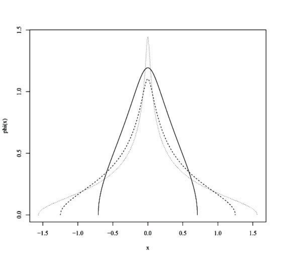
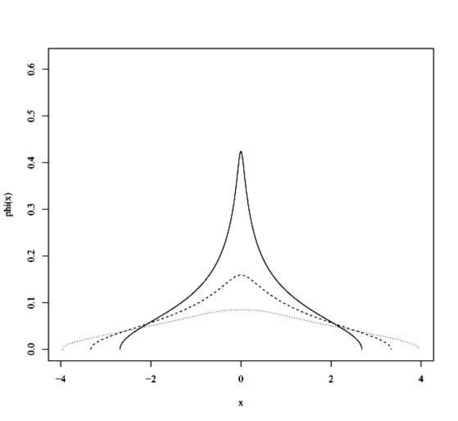
Figures 1 and 2 display the density functions $\phi_{c}(x)$ with $c<1$ and $c>1$, respectively. From these two figures, it is shown that as $c$ increases, the support of $\phi_{c}(x)$ gets wider, and $\phi_{c}(x)$ achieves the maximum at $x=0$ which is sharper as $c$ gets closer to 1.

The goal of the paper is devoted to giving a more direct method of deriving (4), by using Theorem 4.1 in Bai and Silverstein (2010). It is worth noting that for our method to work, we only require the finiteness of the 2nd moment of the underlying random variable, which is weaker than the finite $(2+\delta)$-th moment requirement in Jin et al. (2014). Once (4) is obtained, Theorem 1.1 will follow by employing the technique in Jin et al. (2014) and thus will not be presented again.

Before proceeding, it is necessary to rewrite ${\bf M}_{N}(\tau)$ into another form. For any $\tau\geq 1$ fixed, write

			$\displaystyle{\bf M}_{N}(\tau)$
		$\displaystyle=$	$\displaystyle\sum_{k=1}^{T}({\bf\gamma}_{k}{\bf\gamma}_{k+\tau}^{*}+{\bf\gamma}_{k+\tau}{\bf\gamma}_{k}^{*})$
		$\displaystyle=$	$\displaystyle\frac{1}{2T}\sum_{k=1}^{T}({\bf e}_{k}{\bf e}_{k+\tau}^{*}+{\bf e}_{k+\tau}{\bf e}_{k}^{*})$
		$\displaystyle=$	$\displaystyle\frac{1}{T}({\bf e}_{1},{\bf e}_{2},\cdots,{\bf e}_{T+\tau-1},{\bf e}_{T+\tau})\begin{pmatrix}0&\cdots&\frac{1}{2}&\cdots&0\\ \vdots&\ddots&0&\frac{1}{2}&\vdots\\ \frac{1}{2}&0&\ddots&0&\frac{1}{2}\\ \vdots&\frac{1}{2}&0&\ddots&\vdots\\ 0&\cdots&\frac{1}{2}&\cdots&0\\ \end{pmatrix}\begin{pmatrix}{\bf e}_{1}^{*}\\ {\bf e}_{2}^{*}\\ \vdots\\ {\bf e}_{T+\tau-1}^{*}\\ {\bf e}_{T+\tau}^{*}\end{pmatrix}$
		$\displaystyle\equiv$	$\displaystyle\frac{1}{T}\textbf{X}_{T}\textbf{C}_{T,\tau}\textbf{X}_{T}^{*},$

where the two bands of $\frac{1}{2}$’s are $\tau-$distance from the main diagonal.

Proof. Fix $n$ and let $\lambda$ be an eigenvalue of $\textbf{C}_{n,\tau}$.
Define $D_{n}=D_{n,\tau}=\det(\lambda\textbf{I}-\textbf{C}_{n,\tau})$ (for simplicity, we omit $\tau$ from the subscript).
When $n<\tau$, all the entries of $\textbf{C}_{n,\tau}$ are 0 and hence we have $D_{n}=\lambda^{n}$. For $n\geq\tau$, expand along the first row, and we have $D_{n}=\lambda D_{n-1}+\frac{(-1)^{\tau}}{2}\tilde{D}_{n-1}.$
Expand along the first column of the matrix wrt $\tilde{D}_{n-1}$, and we have $\tilde{D}_{n-1}=\frac{(-1)^{\tau-1}}{2}D_{n-2}.$
Therefore, for $n\geq\tau$, we have

$\displaystyle D_{n}=\lambda D_{n-1}-\frac{1}{4}D_{n-2}$

Solve the characteristic equation $x^{2}=\lambda x-\frac{1}{4}$ and we have $\lambda_{1,2}=\frac{\lambda\pm\sqrt{\lambda^{2}-1}}{2}$.
Thus, we have, for $n\geq\tau$,

$\displaystyle D_{n}=\lambda^{\tau}(a\lambda_{1}^{n-\tau}+b\lambda_{2}^{n-\tau}),$

where $a,b$ can be determined by $D_{\tau}$ and $D_{\tau+1}$, i.e.

	$\displaystyle\lambda^{\tau}$	$\displaystyle=$	$\displaystyle\lambda^{\tau}(a+b)$
	$\displaystyle\lambda^{\tau+1}-\frac{\lambda^{\tau-1}}{4}$	$\displaystyle=$	$\displaystyle\lambda^{\tau}(a\lambda_{1}+b\lambda_{2}).$

Substitute $a,b$ into the equation $D_{n}=0$ and use the facts that $\lambda_{1}+\lambda_{2}=\lambda$ and $\lambda_{1}\lambda_{2}=\frac{1}{4}$, we have

$$\frac{\lambda^{\tau-1}(\lambda_{1}^{n-\tau+2}-\lambda_{2}^{n-\tau+2})}{\lambda_{1}-\lambda_{2}}=0.$$

Therefore, if $\lambda\neq 0$, we must have

$$\Big(\frac{\lambda_{2}}{\lambda_{1}}\Big)^{n-\tau+2}=1,\quad\lambda_{1}\neq\lambda_{2},$$

from which we obtain $\frac{\lambda_{2}}{\lambda_{1}}=\cos\frac{2k\pi}{n-\tau+2}+i\sin\frac{2k\pi}{n-\tau+2}$, $k=1,2,\cdots,n-\tau+1$ ($k=0$ corresponds to the case $\lambda_{1}=\lambda_{2}$ and thus is rejected).
Hence, among the $n$ eigenvalues of $\textbf{C}_{n,\tau}$, $\tau-1$ of them are 0 and the rest $n-\tau+1$ are

$$\lambda=\lambda_{1}+\lambda_{2}=\cos\frac{k\pi}{n-\tau+2},\quad k=1,2,\cdots,n-\tau+1.$$

Define a uniform random variable $K$ taking values in $\{1,2,\cdots,n-\tau+1\}$. Then we have

	$\displaystyle\textrm{P}(\lambda\leq t)$	$\displaystyle=$	$\displaystyle\frac{\tau-1}{n}I_{[0,\infty)}(t)+\frac{n-\tau+1}{n}\textrm{P}\Big(\frac{K}{n-\tau+2}\geq\frac{\cos^{-1}(t)}{\pi}\Big)$
		$\displaystyle\to$	$\displaystyle 1-\frac{\cos^{-1}(t)}{\pi}=:H(t),\quad t\in(-1,1)$

since $\frac{K}{n-\tau+2}\overset{D}{\rightarrow}\textrm{Uniform}(0,1)$ as $n\to\infty$.
Taking the derivative, we have

$$H^{\prime}(t)=\frac{1}{\pi\sqrt{1-t^{2}}},\quad t\in(-1,1).$$

The proof of the lemma is complete.

To derive the Stieltjes transform, we mainly use Theorem 4.1 in Bai and Silverstein (2010).

Also, according to (4.4.4) in Bai and Silverstein (2010),

$\displaystyle\frac{1}{z}m_{F}\Big(\frac{1}{z}\Big)=\frac{1}{y}-1+\frac{1}{2\pi iyz}\oint_{|\zeta|=\rho}\log\Big(1-z\zeta^{-1}+zy\zeta^{-1}+\zeta^{-2}zym_{H}\Big(\frac{1}{\zeta}\Big)\Big)d\zeta.$

(7)

Replacing $z^{-1}$ by $z$, we have

$\displaystyle zm_{F}(z)=\frac{1}{y}-1+\frac{z}{2\pi iy}\oint_{|\zeta|=\rho}\log\Big(z-\zeta^{-1}+y\zeta^{-1}+\zeta^{-2}ym_{H}\Big(\frac{1}{\zeta}\Big)\Big)d\zeta,$

(8)

where we have used the fact that the integral for $\log z$ with respect to $\zeta$ on the contour $|\zeta|=\rho$ is 0.
Next, set $\psi(u)=-\frac{1}{u}+y\int\frac{t}{1+tu}dH(t)$. Then (8) becomes

	$\displaystyle zm_{F}(z)$	$\displaystyle=$	$\displaystyle\frac{1}{y}-1+\frac{z}{2\pi iy}\oint_{|\zeta|=\rho}\log(z-\psi(-\zeta))d\zeta$		(9)
		$\displaystyle=$	$\displaystyle\frac{1}{y}-1-\frac{z}{2\pi iy}\oint_{|\zeta|=\rho}\frac{\zeta}{z-\psi(-\zeta)}d\psi(-\zeta)$
		$\displaystyle=$	$\displaystyle\frac{1}{y}-1-\frac{z}{2\pi iy}\oint_{\mathcal{C}}\frac{\psi^{-1}(s)}{z-s}ds.$

When $\zeta$ is in the contour $|\zeta|=\rho$ with $\rho\in(0,1/\tau_{0})$, where $\tau_{0}$ is a truncation point of eigenvalues of $T_{n}$ as defined in Section 4.3.1 in Bai and Silverstein (2010) and here we can take $\tau_{0}=1+\varepsilon$ for some $\varepsilon>0$ by Lemma 3.1, we have $\psi^{-1}(s)=-\zeta$ being bounded. Therefore, we have $s=z$ as the only pole.
Moreover, as the contour $\mathcal{C}$ is the image of the contour $|\zeta|=\rho$ under the map $\zeta\mapsto\psi(-\zeta)$ and note that $\zeta$ lies on a small circle enclosing the origin. Hence, $\mathcal{C}$ encloses the whole complex plane except a small region containing the origin. Also, by Silverstein and Bai (1995), for each $z\in\mathds{C}^{+}\equiv\{z\in\mathds{C}:\Im(z)>0\}$, there exists a unique solution $\xi\in\mathds{C}^{+}$ such that $z=\psi(-\xi)$. By taking $\tau_{0}$ large enough, we have $s=z$ in the contour $\mathcal{C}$. Therefore,

$\displaystyle zm_{F}(z)=\frac{1}{y}-1+\frac{z}{y}\psi^{-1}(z),$

or equivalently,

$\displaystyle z=\psi(ym_{F}+\frac{y-1}{z}).$

(10)

Note that

	$\displaystyle\psi(u)$	$\displaystyle=$	$\displaystyle-\frac{1}{u}+y\int\frac{t}{1+tu}dH(t)$
		$\displaystyle=$	$\displaystyle\frac{y-1}{u}-\frac{y}{\pi u}\int_{-1}^{1}\frac{1}{(1+tu)\sqrt{1-t^{2}}}dt$
		$\displaystyle=$	$\displaystyle\frac{y-1}{u}-\frac{y}{2\pi u}\int_{0}^{2\pi}\frac{1}{1+u\cos\theta}d\theta$
		$\displaystyle=$	$\displaystyle\frac{y-1}{u}-\frac{y}{2\pi ui}\oint_{|s|=1}\frac{2}{us^{2}+2s+u}ds.$

The integrand has two poles at $s_{1}=\frac{-1+\sqrt{1-u^{2}}}{u}$ and $s_{2}=\frac{-1-\sqrt{1-u^{2}}}{u}$. As $s_{1}s_{2}=1$, we must have one of them is inside the contour and the other is outside. Therefore, we have

	$\displaystyle\psi(u)$	$\displaystyle=$	$\displaystyle\frac{y-1}{u}-\frac{y}{2\pi ui}\oint_{|s|=1}\frac{2}{us^{2}+2s+u}ds$
		$\displaystyle=$	$\displaystyle\frac{y-1}{u}\pm\frac{2y}{u^{2}(s_{1}-s_{2})}$
		$\displaystyle=$	$\displaystyle\frac{y-1}{u}\pm\frac{y}{u\sqrt{1-u^{2}}},$

where the choice of $+$ or $-$ sign is determined by which of $s_{1,2}$ is inside the contour. Substitute the above expression into (8), and we have

$\displaystyle m_{F}^{2}z^{2}[1-(ym_{F}+\frac{y-1}{z})^{2}]=1.$

Note that in our question, $c=\lim_{N\to\infty}N/T=1/y$. Therefore, the Stieltjes transform $\widetilde{m}$ of the LSD of $\widetilde{{\bf M}}_{N}=\frac{1}{N}\textbf{X}_{T}^{*}\textbf{X}_{T}\textbf{C}_{T,\tau}$ satisfies

$\displaystyle\widetilde{m}^{2}z^{2}[1-(\frac{\widetilde{m}}{c}+\frac{1/c-1}{z})^{2}]=1.$

Next, the Stieltjes transform $\underline{m}$ of the LSD of $\underline{{\bf M}}_{N}=\frac{1}{N}\textbf{X}_{T}\textbf{C}_{T,\tau}\textbf{X}_{T}^{*}$ satisfies $\underline{m}=\frac{\widetilde{m}}{c}+\frac{1/c-1}{z}$ and therefore,

$\displaystyle(c\underline{m}-\frac{1-c}{z})^{2}z^{2}(1-\underline{m}^{2})=1.$

Finally, the Stieltjes transform $m$ of LSD of ${\bf M}_{N}=\frac{1}{T}\textbf{X}_{T}\textbf{C}_{T,\tau}\textbf{X}_{T}^{*}$ satisfies

$\displaystyle m(z)$

$\displaystyle=$

$\displaystyle\lim_{N\to\infty}\frac{1}{N}\sum_{i=1}^{N}\frac{1}{\lambda_{i}-z}=\lim_{N\to\infty}\frac{1}{N}\sum_{i=1}^{N}\frac{1}{\frac{N}{T}\underline{\lambda}_{i}-z}=\lim_{N\to\infty}\frac{1}{cN}\sum_{i=1}^{N}\frac{1}{\underline{\lambda}_{i}-\frac{1}{c}z}=\frac{1}{c}\underline{m}(\frac{z}{c}).$

Substituting back to the above equation, we have

$\displaystyle(czm(z)+c-1)^{2}(1-c^{2}m^{2}(z))=1,$

which is the same as (4).

References

• [1] Bai, J. and Ng, S. (2002) Determining the number of factors in approximate factor models. Econometrica 70(1), 191–221.
• [2] Bai, Z. D. and Silverstein, J. W. (2010) Spectral Analysis of Large Dimensional Random Matrices, 2nd ed. Springer Verlag, New York.
• [3] Bai, Z. D. and Silverstein, J. W. (2012) No Eigenvalues Outside the Support of the Limiting Spectral Distribution of Information-Plus-Noise Type Matrices. Random Matrices: Theory and Applications 1, 1150004.
• [4] Bai, Z. D. and Yao, J. F. (2008) Central limit theorems for eigenvalues in a spiked population model. Ann. Inst. H. Poincare Probab. Statist. Volume 44, Number 3, 447–474.
• [5] Baik, Jinho and Silverstein, J. W. (2006) Eigenvalues of large sample covariance matrices of spiked population models. J. Multivariate Anal. 97(6), 1382–1408.
• [6] Dozier, R. B. and Silverstein, J. W. (2007a) On the Empirical Distribution of Eigenvalues of Large Dimensional Information-Plus-Noise Type Matrices. J. Multivariate Anal. 98(4), 678–694.
• [7] Dozier, R. B. and Silverstein, J. W. (2007b) Analysis of the Limiting Spectral Distribution of Large Dimensional Information-Plus-Noise Type Matrices. J. Multivariate Anal. 98(6), 1099–1122.
• [8] Harding, M. C. (2012) Estimating the number of factors in large dimensional factor models. Under Review.
• [9] Jin, B. S., Wang, C., Bai, Z. D., Nair, K. K. and Harding, M. C. (2014) Limiting spectral distribution of a symmetrized auto-cross covariance matrix. Ann. Appl. Probab. (To appear)
• [10] Johnstone, I. (2001) On the distribution of the largest eigenvalue in principal components analysis. Ann. Statist. 29, 295–327.
• [11] Marčenko, V. A. and Pastur, L. A. (1967) Distribution of eigenvalues for some sets of matrices. Mat. Sb. 72, 507–536.
• [12] Silverstein, J. W., and Bai, Z. D. (1995) On the empirical distribution of eigenvalues a class of large dimensional random matrices. J. Multivariate Anal. 54, 175–192.
KLASMOE and School of Mathematics and Statistics, Northeast Normal University, P.R.C, Changchun 130024
Email: baizd@nenu.edu.cn
Department of Statistics and Applied Probability, National University of Singapore, Singapore 117546
Email: wangchen2351@gmail.com