Theoretical Evaluation of Offloading through Wireless LANs

We conducted a significance test of the null hypothesis of a homogeneous Poisson process. We divided the entire region into subregions and counted the number of APs in each region. Let $a_{i}(j)$ be the number of APs provided by the $j$-th operator in the $i$-th subregion, $A_{j}$ be the sample mean of the number of APs provided by the $j$-th operator ($A_{j}\stackrel{{\scriptstyle\mathrm{def}}}{{=}}\sum_{i=1}^{n_{a}}a_{i}(j)/n_{a}$), and $V_{j}$ be its sample variance($V_{j}\stackrel{{\scriptstyle\mathrm{def}}}{{=}}\sum_{i=1}^{n_{a}}(a_{i}(j)-A_{j}))^{2}/(n_{a}-1)$), where $n_{a}$ is the number of subregions. The index of dispersion $I_{d}(j)$ proposed by Sachs was applied to the WLAN APs deployed by the $j$-th operator: $I_{d}(j)\stackrel{{\scriptstyle\mathrm{def}}}{{=}}(n_{a}-1)V_{j}/A_{j}$ (p.54 in [6]). For a significance test of the null hypothesis of a homogeneous Poisson process, $I_{d}(j)$ follows a $\chi^{2}$ distribution with the $n_{a}-1$ degree of freedom ([6], p.104 in [5]). The index $I_{d}$ for each operator and two-side 5% bounds of $\chi^{2}$ for the hypothesis of a homogeneous Poisson process are plotted in Fig. 2. The results in Fig. 2 indicate that we can reject the hypothesis of a homogeneous Poisson process of significance level 0.05. That is, $\{{\bf w}_{i}\}_{i}$ is more clustered than a homogeneous Poisson process, where ${\bf w}_{i}$ is the location of the $i$-th WLAN AP.

By carefully observing the maps in Fig. 1, we can see that all three operators have some common sparse regions. These are regions such as parks or shrines; therefore, WLAN APs are not allowed or it is practically impossible to place them in these regions. We should adopt a model that can describe this fact. Similarly, the operators also have busy regions in common, for example, regions around train/subway stations. To evaluate whether there are common sparse/busy regions, the cross-correlations $c(j,k)$ of $\{a_{i}(j)\}_{i}$ and $\{a_{i}(k)\}_{i}$ were evaluated, where $c(j,k)$ is defined as follows: $c(j,k)\stackrel{{\scriptstyle\mathrm{def}}}{{=}}\frac{\sum_{i}(a_{i}(j)-A_{j})(a_{i}(k)-A_{k})}{(n_{a}-1)\sqrt{V_{j}V_{k}}}$. Figure 3 shows that there are non-negligible cross correlations, particularly between (b) and (c) and between (c) and (a).

Spatial point process models can be classified into two types. In the first type, the placement of WLAN APs is assumed to be mainly determined by the locations of other WLAN APs. We call these internal models. Typical examples of internal models are Matern, simple sequential inhibition, and Gibbs point processes [4],[6]. In the other type, which we call external models, the placement of APs is assumed to be mainly determined by the location features of the APs themselves, rather than the locations of other APs. An inhomogeneous Poisson process, i.e., a Poisson process with inhomogeneous intensity, is a typical example of an external model. Because an inhomogeneous Poisson process model is one in which each point location is determined independently of the other point locations (unlike the other typical models described above), we adopt an inhomogeneous Poisson process as a spatial point process model for $\{{\bf w}_{i}\}_{i}$. In practice, it is impossible for us to reject the internal model based on the data that we have. However, because of this cross-correlation analysis and the fact that the high- or low-density subregions are closely related to the existence of facilities there, we assume the approximation that the WLAN AP locations follow an inhomogeneous Poisson process with intensity $\lambda({\bf x})$, where $\lambda({\bf x})$ is the function of location ${\bf x}$.

Assuming that $\{{\bf w}_{i}\}_{i}$ follow an inhomogeneous Poisson process, the later sections analyze, derive, and evaluate performance metrics, such as mean available bandwidth for a user and the number of vertical handovers through integral geometry.

In the remainder of this paper, $\|X\|$ denotes the size of $X$, $|X|$ denotes the perimeter length of $X$, $\partial X$ denotes the boundary of $X$, and $\overline{X}$ denotes the complementary set (region) of $X$ for region $X\subset\mathbb{R}^{2}$. In addition, for a given line $G$, $\sigma(X)$ denotes the length of the chord $X\cap G$. For regions $X,Y\subset\mathbb{R}^{2}$, $l_{\partial X\cap Y}$ denotes the length of the arc created by $\partial X$ and $Y$, that is, the part of $\partial X$ included in $Y$.

We introduce the concepts of integral geometry and geometric probability [19] as a preliminary to the following analysis.

Consider a bounded set $X\subset\mathbb{R}^{2}$ and a condition $X_{c}$. A typical example of $X_{c}$ is $X_{c}=\{X\cap X_{1}\neq\emptyset\}$ for a given set $X_{1}$. Here, $X$ is, for example, a region covered by a WLAN AP and $X_{1}$ is the cell of a cellular network. Integral geometry provides a method for measuring the expectation of the quantity $q(X)$ for the set of positions of $X$ satisfying a condition $X_{c}$. Then, if we would like to consider the size of the intersection of $X$ and $X_{1}$ when $X$ intesects $X_{1}$, set $q(X)=\|X\cap X_{1}\|$ and $X_{c}=\{X\cap X_{1}\neq\emptyset\}$.

For a set of $X$ whose position is defined by the reference point $(x,y)$ and the angle $\theta$ that a reference line fixed in $X$ makes with another reference line fixed to the fixed coordinates, integral geometry defines $E[q(X)]$ by $\int_{X_{c}}q(X)dX/\int_{X_{c}}dX=\int_{X_{c}}q(X)dx\,dy\,d\theta/\int_{X_{c}}dx\,dy\,d\theta$. The numerator means the integral of $q(X)$ at a position $(x,y,\theta)$ uniformly over the possible parameter space $(x,y,\theta)$ satisfying $X_{c}$, and the denominator means the area size of the parameter space $(x,y,\theta)$ satisfying $X_{c}$. That is, the numerator is (roughly speaking) a summation of $q(X)$ at every points specified by $(x,y,\theta)$ satisfying $X_{c}$, and the denominator is (roughly speaking) the number of points satisfying $X_{c}$. Therefore, it is an expectation of $q(X)$.

In particular, if $q(X)={\bf 1}$ (the position $(x,y,\theta)$ satisfies $Y_{c}$) where ${\bf 1}(\cdot)$ denotes the indicator function and $Y_{c}\subseteqq X_{c}$, $E[q(X)]=\int_{Y_{c}}dx\,dy\,d\theta/\int_{X_{c}}dx\,dy\,d\theta=\Pr(Y_{c}|X_{c})$ is the (conditional) probability of the positions of $X$ satisfying a condition $Y_{c}$ among the positions of $X$ satisfying a condition $X_{c}$. (This is called a geometric probability [19].) In this sense, $\int_{Y_{c}}dx\,dy\,d\theta$ is a non-normalized probability, because it is proportional to the probability and normalized by $\int_{X_{c}}dx\,dy\,d\theta$. In the remainder of this paper, this non-normalized probability is called the measure of the set of positions of $X$ satisfying a condition $Y_{c}$.

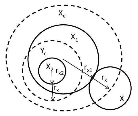
A simple example is shown in Fig. 4, where $X$ is a disk of radius $r_{x}$, $X_{c}=\{X\cap X_{1}\neq\emptyset\}$, $X_{1}$ is a disk of radius $r_{x1}$, $Y_{c}=\{X\cap X_{2}\neq\emptyset\}$, and $X_{2}\subset X_{1}$ is a disk of radius $r_{x2}$. Because this example is independent of $\theta$, we can easily draw a picture. Because integral geometry implicitly assumes that the position $(x,y,\theta)$ uniformly moves in the parameter space (if not explicitly indicated otherwise), we can easily understand that $\Pr(Y_{c}|X_{c})$ is given by $\int_{Y_{c}}dx\,dy\,d\theta/\int_{X_{c}}dx\,dy\,d\theta=\int_{Y_{c}}dx\,dy/\int_{X_{c}}dx\,dy=(r_{x2}+r_{x})^{2}/(r_{x1}+r_{x})^{2}$.

When $X$ is a line $G$, we should use the parameterization by the angle $\theta$, in which the direction perpendicular to $G$ is a fixed direction ($-\pi\leq\theta\leq\pi$), and by its distance $p$ from the origin $O$ ($0\leq p$). (We can use another parameterization, but we cannot calculate the integral uniformly over the possible parameter space $X_{c}$ when the parameters $\theta$ and $p$ are not used. This is because integral geometry requires the calculated results to be invariant under the group of motions in the plane.) By using $\theta$ and $p$, the expectation of the quantity $q(G)$ satisfying $X_{c}$ can be calculated by $\int_{X_{c}}q(G)dG/\int_{X_{c}}dG=\int_{X_{c}}q(G)dp\,d\theta/\int_{X_{c}}dp\,d\theta$.

In Section VI-B, we assume that a user moves on $G$. By defining $X_{c}$ such that $G$ intersects the cell and setting $q(G)$ as the chord length of $G$ in the cell, we can calculate the mean distance (that is, the mean length of the chord) that a user moves in the cell.

The following basic formulas are known or directly derived through integral geometry.

Accoring to Eqs. (3.12) and (3.6) in [19], for a fixed convex set $K$, the measure in which the set of positions of a line $G$ that meets $K$ is given by

and the (non-normalized) mean length of the chord made by $\partial K$ and $G$ is given by

For a fixed convex set $K_{0}$, the measure of the set of positions of a convex set $K_{1}$ that meets $K_{0}$ is given as follows (Eq. (6.48) in [19]).

where $f(X,Y)\stackrel{{\scriptstyle\mathrm{def}}}{{=}}2\pi(\|X\|+\|Y\|)+|X|\cdot|Y|$.

Particularly when $K_{0}$ is a point, Eq. (3) becomes

For a fixed convex set $K_{0}$, the measure of the set of positions of a convex set $K_{1}$ that is contained in $K_{0}$ is given as follows (Eq. (6.52) in [19]).

Formally speaking, additional conditions on the curvature of $\partial K_{0}$ and that of $\partial K_{1}$ are needed for Eq. (5) where $\partial K$ for a set $K\subset\mathbb{R}^{2}$ means the boundary of $K$.

For a fixed set $K_{0}$, the integral of $\|K_{0}\cap K_{1}\|$ over the position of the set of $K_{1}$ is given as follows. (Eq. (6) is Eq. (6.57) in [19]. Although Eq. (6.57) in [19] does not include $\pi$, Eqs. (6.55) and (6.56) used in [19] to derive Eq. (6.57) show that Eq. (6) is correct and the original Eq. (6.57) in [19] is incorrect.).

Due to Eq. (6.61) in [19] and Eq. (5), Eq. (9) concerning the integral of $l_{\partial K_{1}\cap K_{0}}$ (the length of the arc of $\partial K_{1}$ intersecting $K_{0}$) is given as follows.

Based on Eq. (6), for any $K_{2}\subset K_{0}$,

This is because (i) $\int_{K_{0}\cap K_{1}\neq\emptyset}\|K_{2}\cap K_{1}\|dK_{1}=\int_{K_{2}\cap K_{1}\neq\emptyset}\|K_{2}\cap K_{1}\|dK_{1}+\int_{K_{2}\cap K_{1}=\emptyset,K_{0}\cap K_{1}\neq\emptyset}\|K_{2}\cap K_{1}\|dK_{1}$, and (ii) the second term is 0 due to $\|K_{2}\cap K_{1}\|=0$ for $K_{2}\cap K_{1}=\emptyset$.

To analyze an inhomogeneous Poisson process, we propose the following extensions for the basic formulas mentioned above. We assume that $\Omega$ is a convex set and that $dK_{1}=d{\bf w}\ d\gamma$ where ${\bf w}$ is a reference point in $K_{1}$, and $\gamma$ is the angle characterizing $K_{1}$. These extensions require that the reference point ${\bf w}$ must be within $\Omega$. For a fixed $K_{0}$, the relative location of $\Omega$ is assumed to be fixed. In the following, the term $\hat{r}(K_{1})$ is similar to the radius of $K_{1}$, and we adopt the definition $\hat{r}(K_{1})\stackrel{{\scriptstyle\mathrm{def}}}{{=}}|K_{1}|/(2\pi)$. This term is identical to the radius when $K_{1}$ is a disk.

Eqs. (3) and (5) are approximately extended to the following. For a fixed convex set $K_{0}$, the measure of the set of positions of a convex set $K_{1}$ that meets $K_{0}$ and is contained in $K_{0}$ are given as follows.

This is due to Fig. 5-(a), (b) where the gray regions indicate where ${\bf w}$ can exist. Thus, the right-hand sides of Eqs. (11) and (12) are approximations of the size of these regions times 2$\pi$.

When $K_{0}$ is a point, the following approximation, which is an analogy of Eq. (4), is proposed.

Eq. (6) is approximately extended to the following. For a fixed set $K_{0}$, the integral of $\|K_{0}\cap K_{1}\|$ and the integral of $l_{\partial K_{1}\cap K_{0}}$ over positions of a set $K_{1}$ are given as follows.

This is due to Fig. 5-(c). Here, $\|K_{0}\cap K_{1}\|$ becomes $\|K_{1}\|$ for ${\bf w}$ in the black region in this figure, and it becomes approximately half of $\|K_{1}\|$ for ${\bf w}$ in the gray region. The size of the black region is approximately $\|K_{0}\cap\Omega\|-\hat{r}(K_{1})l_{\partial K_{0}\in\Omega}$ and that of the gray region is approximately $2\hat{r}(K_{1})l_{\partial K_{0}\in\Omega}$. Therefore, we obtain Eq. (15).

Applying Eq. (15), for any $K_{2}\subset K_{0}$,

Eq. (9) is approximately extended to the following. Because $l_{\partial K_{1}\cap K_{0}}\approx|K_{1}|/2$ and $\int_{\partial K_{0}\cap K_{1}\neq\emptyset,{\bf w}\in\Omega}d{\bf w}\approx 2\hat{r}(K_{1})l_{\partial K_{0}\cap\Omega}$,

Eqs. (11), (12), (15) (as a result, Eq. (16)), and (17) are exact when $\partial K_{0}$ is a line segment in $\Omega$, $K_{1}$ is a disk with radius $r_{K_{1}}$, and $\partial\Omega\subset(\overline{K_{0}}\cap(K_{0}\oplus r_{K_{1}}))$ is a line segment vertical to $\partial K_{0}$ where $K_{0}\oplus r_{K_{1}}$ is a Minkoski sum of $K_{0}$ and a disk with radius $r_{K_{1}}$.

This subsection provides $B_{s}$ and $q_{s}(x)$. First, we evaluate the expected area size of $C_{j}\cap_{m=i_{1},\cdots,i_{k}}D_{m}$ under the condition $\{C\cap D_{i}\neq\emptyset\}_{i=1}^{l}$. Second, by describing $p_{j}$, which is the probability that the point is in $C_{j}-C_{j+1}$ and is covered by at least a single WLAN, with this expected area size, we derive $p_{j}$. Third, based on $p_{j}$, $B_{s}$ and $q_{s}(x)$ are derived.

References

• [1] Y. Choi, H. W. Ji, J.-Y, Park, H.-C Kim, and J. A. Silvester, A 3W Network Strategy for Mobile Data Traffic Offloading, IEEE Communications Magazine, 49, 10, pp. 118-123, 2011.
• [2] A. de la Oliva, C. J. Bernardos, M. Calderon, T. Melia, and J. C. Zuniga, IP Flow Mobility: Smart Traffic Offload for Future Wireless Networks, IEEE Communications Magazine, 49, 10, pp. 124-132, 2011.
• [3] C. B. Sankaran, Data Offloading Techniques in 3GPP Rel-10 Networks: A Tutorial, IEEE Communications Magazine, 50, 6, pp.46-53, 2012.
• [4] Noel A. C. Cressie, Statistics for Spatial Data, John Wiley & Sons, 1991.
• [5] B. D. Ripley, Spatial Statistics, John Wiley & Sons, 1981.
• [6] S. Mase and J. Takeda, Spatial Data Modeling, Kyoritsu, 2001 (in Japanese).
• [7] A. Baddeley and R. Turner, spatstat: An R Package for Analyzing Spatial Point Patterns, Journal of Statistical Software, 12, 6, 2005.
• [8] J. Riihijärvi and P. Mähönen, and M. Rübsamen, Characterizing Wireless Networks by Spatial Correlations, IEEE Communication Letters 2007.
• [9] J. Riihijärvi and P. Mähönen, Modeling Spatial Structure of Wireless Communication Networks, NetSciCom 2010, 2010.
• [10] M. Michalopoulou, J. Riihijärvi and P. Mähönen, Studying the Relationships between Spatial Structures of Wireless Networks and Population Densities, IEEE Globecom 2010.
• [11] J. G. Andrews, F. Baccelli, R. K. Ganti, A Tractable Approach to Coverage and Rate in Cellular Networks, IEEE Transactions on Communications 59, 11, pp. 3122-3134, 2011.
• [12] C. Gloaguen, F. Voss, and V. Schmidt, Parametric Distance Distributions for Fixed Access Network Analysis and Planning, 21st International Teletraffic Congress (ITC21), Paris, 2011.
• [13] C. Gloaguen, H. Schmidt, R. Thiedmannz, J. Lanquetiny, and V. Schmidt, Comparison of Network Trees in Deterministic and Random Settings using Different Connection Rules, Modeling and Optimization in Mobile, Ad Hoc and Wireless Networks and Workshops, 2007.
• [14] H. Saito, K. Shimogawa, S. Shioda, and J. Harada, Shape Estimation Using Networked Binary Sensors, INFOCOM 2009, 2009.
• [15] H. Saito, S. Tanaka, and S. Shioda, Estimating Parameters of Multiple Heterogeneous Target Objects Using Composite Sensor Nodes, IEEE Trans. Mobile Computing, 11, 1, pp. 125-138, 2012.
• [16] H. Saito, S. Tanaka, and S. Shioda, Stochastic Geometric Filter and its Application to Shape Estimation for Target Objects, IEEE Trans. Signal Processing, 59, 10, pp. 4971-4984, 2011.
• [17] L. Lazos, R. Poovendran, and J. A. Ritcey, Probabilistic Detection of Mobile Targets in Heterogeneous Sensor Networks, IPSN07, pp. 519–528, 2007.
• [18] L. Lazos and R. Poovendran, Stochastic Coverage in Heterogeneous Sensor Networks, ACM Transactions on Sensor Networks, 2, 3, pp. 325–358, 2006.
• [19] L. A. Santaló, Integral Geometry and Geometric Probability, Second edition. Cambridge University Press, Cambridge, 2004.
• [20] S. Kwon and N. B. Shroff, Analysis of Shortest Path Routing for Large Multi-Hop Wireless Networks, IEEE/ACM Trans. Networking, 17, 3, pp. 857–869, 2009.
• [21] W. Choi and S. K. Das, A Novel Framework for Energy-Conserving Data Gathering in Wireless Sensor Networks, INFOCOM 2005, pp. 1985–1996, 2005.
• [22] S. Neumayer and E. Modiano, Network Reliability With Geographically Correlated Failures, INFOCOM 2010, 2010.
• [23] H. Saito, Disaster Evaluation Model for Networks and its Analysis, submitted for publication.
• [24] livedoor public wireless LAN internet access service site (in Japanese): http://wireless.livedoor.com/map/ [Last access: 2 Oct., 2013].
• [25] NTT East FLET’s public wireless LAN internet access service site (in Japanese):
http://flets.com/spot/ap/ap_search_s.html [Last access: 2 Oct., 2013].
• [26] SoftBank public wireless LAN internet access service site (in Japanese):
http://mb.softbank.jp/mb/service_area/sws/ [Last access: 2 Oct., 2013].
• [27] K. I. Pedersen, T. E. Kolding, F. Frederiksen, I. Z. Kovacs, D. Laselva, and P. E. Mogensen, An Overview of Downlink Radio Resource Management for UTRAN Long-Term Evolution, IEEE Communications Magazine, pp. 86-93, July 2009.
• [28] P. Bhat, S. Nagata, L. Campoy, I. Berberana, T. Derham, G. Liu, X. Shen, P. Zong, and Jin Yang, LTE-Advanced: An Operator Perspective, IEEE Communications Magazine, pp. 104-114, February 2012.
• [29] E. Dahlman, S. Parkvall, J. Skold, and P. Beming, 3G evolution: HSPA and LTE for mobile broadband (2nd edition), Elsevier, UK, 2008.
• [30] J. C. Chen and J. M. Gilbert, Measured Performance of 5-GHz 802.11a Wireless LAN Systems:
http://www.iet.unipi.it/f.giannetti/documenti/wlan/Data/refer/AtherosRangeCapacityPaper.pdf [Last access: 4 Oct., 2013]
• [31] http://en.wikipedia.org/wiki/Wi-Fi
• [32] P. Deshpande, X. Hou, and S. R. Das, Performance Comparison of 3G and Metro-Scale WiFi for Vehicular Network Access, ACM IMC 2010.
• [33] A. Balasubramanian, R. Mahajan, and A. Venkataramani, Augmenting Mobile 3G Using WiFi, ACM MobiSys Conference, 2010.
• [34] R. Gass and C. Diot, An Experimental Performance Comparison of 3G and Wi-Fi, PAM 2010.
• [35] A. L. Wijesinha, Y.-T. Song, M. Krishnan, V. Mathur, J. Ahn, and V. Shyamasundar, Throughput Measurement for UDP Traffic in an IEEE 802.11g WLAN, SNPD/SAWM 2005, May 2005.
Appendix A Proof of Eq. (33)
Because Cj∩Di1∩Di2∩⋯C_{j}\cap D_{i_{1}}\cap D_{i_{2}}\cap\cdots is convex, by applying Eq. (28) for i≠i1,⋯,iki\neq i_{1},\cdots,i_{k},
∫{C∩Di≠∅}i=1l∥Cj∩m=i1,⋯,ikDm∥(dD)l\displaystyle\int_{\{C\cap D_{i}\neq\emptyset\}_{i=1}^{l}}\|C_{j}\cap_{m=i_{1},\cdots,i_{k}}D_{m}\|(dD)^{l} (124)
≈\displaystyle\approx Πi≠i1,⋯,ikρ0g1(C,Di)∫C∩Di1≠∅,⋯,C∩Dik≠∅∥Cj∩m=i1,⋯,ikDm∥dDi1⋯dDik\displaystyle\Pi_{i\neq i_{1},\cdots,i_{k}}\rho_{0}g_{1}(C,D_{i})\int_{C\cap D_{i_{1}}\neq\emptyset,\cdots,C\cap D_{i_{k}}\neq\emptyset}\|C_{j}\cap_{m=i_{1},\cdots,i_{k}}D_{m}\|dD_{i_{1}}\ \cdots\ dD_{i_{k}} (125)
Use Eq. (26) with ϕ=∥Cj∩m=i1,⋯,ikDm∥,Xc={C∩Di≠∅}i=1l\phi=\|C_{j}\cap_{m=i_{1},\cdots,i_{k}}D_{m}\|,X_{c}=\{C\cap D_{i}\neq\emptyset\}_{i=1}^{l}, and apply Eqs. (10) and (16).
∫{C∩Di≠∅}i=1l∥Cj∩m=i1,⋯,ikDm∥dDik\displaystyle\int_{\{C\cap D_{i}\neq\emptyset\}_{i=1}^{l}}\|C_{j}\cap_{m=i_{1},\cdots,i_{k}}D_{m}\|dD_{i_{k}} (126)
=\displaystyle= ρ0{∫{C∩Di≠∅}i=1l,𝐰ik∈ℝ2∥Cj∩m=i1,⋯,ikDm∥d𝐰ikdγik\displaystyle\rho_{0}\{\int_{\{C\cap D_{i}\neq\emptyset\}_{i=1}^{l},{\bf w}_{i_{k}}\in{\mathbb{R}}^{2}}\|C_{j}\cap_{m=i_{1},\cdots,i_{k}}D_{m}\|d{\bf w}_{i_{k}}\ d\gamma_{i_{k}} (129)
+ρH∫{C∩Di≠∅}i=1l,𝐰ik∈ΩH∥Cj∩m=i1,⋯,ikDm∥d𝐰ikdγik\displaystyle+\rho_{H}\int_{\{C\cap D_{i}\neq\emptyset\}_{i=1}^{l},{\bf w}_{i_{k}}\in\Omega_{H}}\|C_{j}\cap_{m=i_{1},\cdots,i_{k}}D_{m}\|d{\bf w}_{i_{k}}\ d\gamma_{i_{k}}
−ρL∫{C∩Di≠∅}i=1l,𝐰ik∈ΩL∥Cj∩m=i1,⋯,ikDm∥d𝐰ikdγik}\displaystyle-\rho_{L}\int_{\{C\cap D_{i}\neq\emptyset\}_{i=1}^{l},{\bf w}_{i_{k}}\in\Omega_{L}}\|C_{j}\cap_{m=i_{1},\cdots,i_{k}}D_{m}\|d{\bf w}_{i_{k}}\ d\gamma_{i_{k}}\}
≈\displaystyle\approx 2πρ0∥Dik∥(∥Cj∩m=i1,⋯,ik−1Dm∥\displaystyle 2\pi\rho_{0}\|D_{i_{k}}\|(\|C_{j}\cap_{m=i_{1},\cdots,i_{k-1}}D_{m}\| (131)
+ρH∥Cj∩m=i1,⋯,ik−1Dm∩ΩH∥−ρL∥Cj∩m=i1,⋯,ik−1Dm∩ΩL∥).\displaystyle\qquad+\rho_{H}\|C_{j}\cap_{m=i_{1},\cdots,i_{k-1}}D_{m}\cap\Omega_{H}\|-\rho_{L}\|C_{j}\cap_{m=i_{1},\cdots,i_{k-1}}D_{m}\cap\Omega_{L}\|).
Again, due to Eqs. (10), (16), and (26),
∫{C∩Di≠∅}i=1l∥Cj∩m=i1,⋯,ik−1Dm∩ΩH∥dDik−1\displaystyle\int_{\{C\cap D_{i}\neq\emptyset\}_{i=1}^{l}}\|C_{j}\cap_{m=i_{1},\cdots,i_{k-1}}D_{m}\cap\Omega_{H}\|dD_{i_{k-1}} (132)
≈\displaystyle\approx 2πρ0∥Dik−1∥(∥Cj∩m=i1,⋯,ik−2Dm∩ΩH∥+ρH∥Cj∩m=i1,⋯,ik−2Dm∩ΩH∥)\displaystyle 2\pi\rho_{0}\|D_{i_{k-1}}\|(\|C_{j}\cap_{m=i_{1},\cdots,i_{k-2}}D_{m}\cap\Omega_{H}\|+\rho_{H}\|C_{j}\cap_{m=i_{1},\cdots,i_{k-2}}D_{m}\cap\Omega_{H}\|) (133)
=\displaystyle= 2πρ0(1+ρH)∥Dik−1∥⋅∥Cj∩m=i1,⋯,ik−2Dm∩ΩH∥,\displaystyle 2\pi\rho_{0}(1+\rho_{H})\|D_{i_{k-1}}\|\cdot\|C_{j}\cap_{m=i_{1},\cdots,i_{k-2}}D_{m}\cap\Omega_{H}\|, (134)
because ΩH∩ΩH=ΩH\Omega_{H}\cap\Omega_{H}=\Omega_{H} and ΩH∩ΩL=∅\Omega_{H}\cap\Omega_{L}=\emptyset. Therefore,
∫{C∩Di≠∅}i=1l∥Cj∩m=i1,⋯,ik−1Dm∩ΩH∥dDi1⋯dDik−1\displaystyle\int_{\{C\cap D_{i}\neq\emptyset\}_{i=1}^{l}}\|C_{j}\cap_{m=i_{1},\cdots,i_{k-1}}D_{m}\cap\Omega_{H}\|dD_{i_{1}}\cdots dD_{i_{k-1}} (135)
≈\displaystyle\approx {2​π​ρ0​(1+ρH)}k−1​Πm=1k−1​‖Dim‖⋅‖Cj∩ΩH‖.\displaystyle\{2\pi\rho_{0}(1+\rho_{H})\}^{k-1}\Pi_{m=1}^{k-1}\|D_{i_{m}}\|\cdot\|C_{j}\cap\Omega_{H}\|. (136)
Similarly,
∫{C∩Di≠∅}i=1l∥Cj∩m=i1,⋯,ik−1Dm∩ΩL∥dDi1⋯dDik−1\displaystyle\int_{\{C\cap D_{i}\neq\emptyset\}_{i=1}^{l}}\|C_{j}\cap_{m=i_{1},\cdots,i_{k-1}}D_{m}\cap\Omega_{L}\|dD_{i_{1}}\cdots dD_{i_{k-1}} (137)
≈\displaystyle\approx {2​π​ρ0​(1−ρL)}k−1​Πm=1k−1​‖Dim‖⋅‖Cj∩ΩL‖.\displaystyle\{2\pi\rho_{0}(1-\rho_{L})\}^{k-1}\Pi_{m=1}^{k-1}\|D_{i_{m}}\|\cdot\|C_{j}\cap\Omega_{L}\|. (138)
Hence,
∫{C∩Di≠∅}i=1l∥Cj∩m=i1,⋯,ikDm∥dDi1⋯dDik\displaystyle\int_{\{C\cap D_{i}\neq\emptyset\}_{i=1}^{l}}\|C_{j}\cap_{m=i_{1},\cdots,i_{k}}D_{m}\|dD_{i_{1}}\ \cdots\ dD_{i_{k}} (139)
≈\displaystyle\approx 2πρ0∥Dik∥∫C∩Di1≠∅,⋯,C∩Dik−1≠∅∥Cj∩m=i1,⋯,ik−1Dm∥dDi1⋯dDik−1\displaystyle 2\pi\rho_{0}\|D_{i_{k}}\|\int_{C\cap D_{i_{1}}\neq\emptyset,\cdots,C\cap D_{i_{k-1}}\neq\emptyset}\|C_{j}\cap_{m=i_{1},\cdots,i_{k-1}}D_{m}\|dD_{i_{1}}\ \cdots\ dD_{i_{k-1}} (141)
+ρH​(1+ρH)k−1​Πm=1k​(2​π​ρ0​‖Dim‖)​‖Cj∩ΩH‖−ρL​(1−ρL)k−1​Πm=1k​(2​π​ρ0​‖Dim‖)​‖Cj∩ΩL‖.\displaystyle\qquad+\rho_{H}(1+\rho_{H})^{k-1}\Pi_{m=1}^{k}(2\pi\rho_{0}\|D_{i_{m}}\|)\|C_{j}\cap\Omega_{H}\|-\rho_{L}(1-\rho_{L})^{k-1}\Pi_{m=1}^{k}(2\pi\rho_{0}\|D_{i_{m}}\|)\|C_{j}\cap\Omega_{L}\|.
Define
Jk\displaystyle J_{k} =def\displaystyle\stackrel{{\scriptstyle\mathrm{def}}}{{=}} ∫C∩Di1≠∅,⋯,C∩Dik≠∅∥Cj∩m=i1,⋯,ikDm∥dDi1⋯dDik\displaystyle\int_{C\cap D_{i_{1}}\neq\emptyset,\cdots,C\cap D_{i_{k}}\neq\emptyset}\|C_{j}\cap_{m=i_{1},\cdots,i_{k}}D_{m}\|dD_{i_{1}}\ \cdots\ dD_{i_{k}}
−(1+ρH)k​Πm=1k​(2​π​ρ0​‖Dim‖)​‖Cj∩ΩH‖\displaystyle\qquad\qquad-(1+\rho_{H})^{k}\Pi_{m=1}^{k}(2\pi\rho_{0}\|D_{i_{m}}\|)\|C_{j}\cap\Omega_{H}\|
−(1−ρL)k​Πm=1k​(2​π​ρ0​‖Dim‖)​‖Cj∩ΩL‖.\displaystyle\qquad\qquad-(1-\rho_{L})^{k}\Pi_{m=1}^{k}(2\pi\rho_{0}\|D_{i_{m}}\|)\|C_{j}\cap\Omega_{L}\|.
Then, the equation above can be described as Jk≈2​π​ρ0​‖Dik‖​Jk−1J_{k}\approx 2\pi\rho_{0}\|D_{i_{k}}\|J_{k-1}. Therefore, Jk≈(2​π​ρ0)k​Πj=1k​‖Dij‖​J0=(2​π​ρ0)k​Πj=1k​‖Dij‖​(‖Cj‖−‖Cj∩ΩH‖−‖Cj∩ΩL‖)J_{k}\approx(2\pi\rho_{0})^{k}\Pi_{j=1}^{k}\|D_{i_{j}}\|J_{0}=(2\pi\rho_{0})^{k}\Pi_{j=1}^{k}\|D_{i_{j}}\|(\|C_{j}\|-\|C_{j}\cap\Omega_{H}\|-\|C_{j}\cap\Omega_{L}\|).
∫{C∩Di≠∅}i=1l∥Cj∩m=i1,⋯,ikDm∥dDi1⋯dDik\displaystyle\int_{\{C\cap D_{i}\neq\emptyset\}_{i=1}^{l}}\|C_{j}\cap_{m=i_{1},\cdots,i_{k}}D_{m}\|dD_{i_{1}}\ \cdots\ dD_{i_{k}} (142)
=\displaystyle= g2​(Cj,k)​Πi=i1,⋯,ik​(2​π​ρ0​‖Di‖)\displaystyle g_{2}(C_{j},k)\Pi_{i=i_{1},\cdots,i_{k}}(2\pi\rho_{0}\|D_{i}\|) (143)
By applying this result to Eq. (125), we obtain Eq. (33).