Batch latency analysis and phase transitions for a tandem of queues with exponentially distributed service times
Abstract
We analyze the latency or sojourn time for the last customer in a batch of customers to exit from the -th queue in a tandem of queues in the setting where the queues are in equilibrium before the batch of customers arrives at the first queue. We first characterize the distribution of exactly for every and , under the assumption that the queues have unlimited buffers and that each server has customer independent, exponentially distributed service times with an arbitrary, known rate. We then evaluate the first two leading order terms of the distributions in the large and limit and bring into sharp focus the existence of phase transitions in the system behavior. The phase transition occurs due to the presence of either slow bottleneck servers or a high external arrival rate. We determine the critical thresholds for the service rate and the arrival rate, respectively, about which this phase transition occurs; it turns out that they are the same. This critical threshold depends, in a manner we make explicit, on the individual service rates, the number of customers and the number of queues but not on the external arrival rate.
1 Introduction
Tandem queues are important models for production systems [31] and communication networks [52]. The fact that the output process of a server is the arrival process for the subsequent queue makes tandem queues difficult to analyze. There are several results in the literature on the waiting time [43] of customers in such queues [24, 47], moment generating functions [23], scaling properties [13], heavy traffic approximations [27] and bounds thereof [50, 36, 37], to list a few. These results capture the behavior of a single randomly selected customer. In this paper, in contrast, we are interested in the latency or sojourn time of a batch of customers entering a system of tandem queues with unlimited buffers that are in equilibrium due to an external arrival process of rate at the first queue before the first customer of the batch arrives; the same setup with was considered by Glynn and Whitt in their seminal paper [25] and more recently by Baccelli, Borovkov and Mairesse in [2]. The batch latency analysis problem is motivated by networking applications such as peer-to-peer sharing where a (large) file is transferred from a source to a destination over a large multi-hop network [14, 16].
This setting is considerably more difficult to analyze at a level that captures what happens as the “wave” of customers traverses the network. Of particular relevance to this work is using the analysis to provide insights on what happens when a few bottleneck servers are particularly slow or when the rate of the external arrival process is relatively large.
In this paper, we leverage recent results from directed last passage percolation (DLPP) and random matrix theory (e.g. [28, 40, 12]) to show that the latency distribution equals that of the largest eigenvalue of a specially constructed random matrix (see Theorem 2.1).
We then employ asymptotics to uncover a phase transition which separates a regime in which the presence of slow bottleneck servers results in a latency that differs from the case where there are no slow servers. It is shown that the leading order of the latency is affected only if the slowest server has the service rate below a critical threshold. We also show that the next order fluctuations change in this case with different order of the variance. The analysis highlights why optimizing the service rates of a limited or number of bottleneck servers might produce asymptotically vanishing gains in the latency reduction achieved.
A similar phase transition occurs with respect to the external arrival rate . In this case the leading order of the latency is affected if is higher than a critical threshold. It is shown that this critical threshold is the same as the one that arises from the slow server phase transition analysis.
The paper is organized as follows. In Section 2, we state the problem addressed in this paper formally and present the main results. Some examples where our results may be applied along with a numerical computation are discussed in Section 3. The proofs of the main results are provided in Sections 4 and 6. Section 5 contains an intuitive explanation for the origin of the phase transition.
2 Main results
2.1 Problem
Consider a tandem of queues associated with servers labeled from left to right as . We assume that each queue is and that the service time at server is exponentially distributed with a customer-independent rate equal to . Each customer starts at queue . After being served by , the customer joins queue and waits for the turn to be served by . After being served, the customer then joins queue and so on until the customer exists queue . We assume that the queue buffers are infinitely long and there are no external arrivals in the system except to queue . The arrival process to the first queue is an independent Poisson process of rate . Suppose that the system is in equilibrium. We assume that for all so that the queues are stable.
Now suppose that we send in a batch of customers to queue . We assume that this arrival is according to the arrival Poisson process: we may think that when a new customer arrives at queue according to the Poisson process, we send in more customers immediately. Let denote the latency or sojourn time for the last of the batch of customers to exit from the last queue . Here the time is measured from the instance when the customers arrive at queue . If we assume that the batch of customers is sent in at an arbitrary time, rather than as a part of the arrival Poisson process, it is easy to see that the asymptotic results in this section still hold even though the exact result, Theorem 2.1, does not hold.
We note that the case corresponds to the setting where the queues are initially empty. The batch of customers are sent into queue and the latency is measured from this point.
2.2 Exact distribution
The standard complex normal distribution is denoted by . The notation means that where and are i.i.d. .
Theorem 2.1 (Exact distribution).
Define the diagonal matrices
Let and denote an matrix and an vector of i.i.d. entries, respectively. Consider the random Hermitian matrix
Then we have that for all and ,
Here denotes the largest eigenvalue of and denotes equality in distribution.
This result follows from interpreting the tandem queues model in terms of directed last passage percolation (DLPP) model [47, 25, 42] and then using a result due to Borodin and Péché [12] on the relation between certain DLPP models and random matrices. See Section 4.
Remark 2.1.
Note that since the normal distribution is rotationally invariant, the distribution of the eigenvalues of is unchanged even if we re-arrange the ordering of ’s. Hence we find that the distribution of does not depend on the ordering of ’s, a fact first proved in [51].
2.3 Asymptotic result I. Leading order
We first introduce some definitions and assumptions. Let
| (1) |
be an ordered re-arrangement of the services rates . Consider the probability measure (the spectral measure for the service rates)
| (2) |
Assume that there is a compactly supported probability measure such that
| (3) |
as (i.e. for all bounded continuous functions .) This includes examples such as (a) for all , (b) and for all , and (c) for for a piecewise-continuous, non-negative and compactly support function with total mass . We denote the support of and by and respectively. Note that the minimum of is .
Define the function
| (4) |
See Figure 1 for an example. It is easy to see that for . Since as and as , there is a unique point such that . We denote this point by ;
| (5) |
Note that for and for .
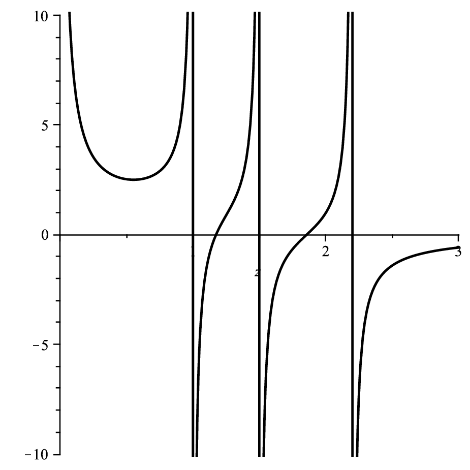
Theorem 2.2 (Asymptotic result I. Leading order).
Assume (3). Let and be defined as in (4)) and (5)) respectively. Recall that is the arrival rate and assume that . From the definition, . The following asymptotic result holds in probability as such that .
- (a)
If and , then
(6) - (b)
If , then
(7) - (c)
Suppose that and there is a fixed (which does not grow in ) such that and . Furthermore, assume that where is the unique real root of the equation in where
(8) Then
(9)
The above theorem can be simplified if we assume that the limit of as exists.
Corollary 2.1 (Easier conditions when ).
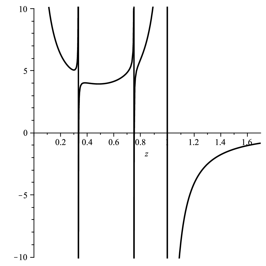
Suppose that as for some . Set
| (10) |
and let be the unique solution to in ;
| (11) |
(Hence is the analogue of with replaced by in (3), and is the analogue of . See Figure 2 for an example.) Then the following asymptotic result holds in probability as such that .
- (i)
If , then .
- (ii)
If , then .
- (iii)
If , and if for some fixed and , then .
Proof.
Note that as weakly, , and hence . If , it is easy to check, using the fact that and using the analyticity of for , that , and also for each . Hence we are in the case (a) or (b) of Theorem 2.2 depending on or , and the above results for (i) and (ii) follow. On the other hand if , then it is also easy to check that for any compact interval of , there is no zero of the equation (5) for all large enough . This means that , and hence we find that the conditions for the case (c) of Theorem 2.2 are satisfied. It is also direct to check that for each since is analytic in any closed interval in this interval for all large enough . Thus the case (iii) follows. ∎

2.4 Asymptotic result II. Second order
The next theorem is about the second order asymptotics. We evaluate the law of the asymptotic fluctuations. Let denote the complex Tracy-Widom random variable from random matrix theory [48]. There are other Tracy-Widom random variables, , and the subscript in signifies that this random variable is related to the so-called complex case in random matrix theory. See (52) below for an explicit formula of and Section 8 for additional information. The notation means convergence in distribution.
Theorem 2.3 (Asymptotic result II. Second order).
Note that the denominator in (12) is while the denominators in (13) and (14) are . Hence the order of the fluctuations in the case (a) is different from the cases (b) and (c).
Remark 2.2.
In the case (c), if and for a fixed , then we have the same scaling but a different limiting distribution. The new distribution is same as the largest eigenvalue of the so-called matrix from the Gaussian unitary ensemble [33].
The above theorem can be simplified as follows under some extra conditions. The proof of this Corollary is similar to the argument in the proof of Corollary 2.2 and we skip it.
2.5 Related results from random matrix theory
Phase transitions have also been studied in random matrix theory, especially for the so-called ‘spiked random matrix’ models. These models are of particular interest for principal component analysis in statistics [30] and in this context the phase transition was first obtained in [4]. By Theorem 2.1, such results in random matrix theory can be interpreted as results for tandem queues. The following cases have been studied:
- (1)
and in [28],
- (2)
- (3)
From Theorem 2.1, one can see that the case when and is almost the same as the case when and only is different from other service rates. Thus, case (2) above also includes the case when
- (4)
and .
For the above case, both the leading order and the second order asymptotics are known. For general ’s, the following cases have been studied:
In this paper we obtain the asymptotic results for the general setting where and are arbitrary. This general case does not follow from existing results in the literature.
3 Examples and discussions
Example 3.1 (Equal service rates, initially empty queues).
Example 3.2 (Equal service rates, queues in equilibrium).
The only change from the previous example is that . Hence case (ii) may occur and we find that
| (22) |
Example 3.2 shows a phase transition phenomenon. When is below the threshold , the latency is same as that of the system with initially empty queues. The existing customers do not contribute to the leading order asymptotic of . (Actually they do not contributed even to the second leading order asymptotic; see Corollary 2.2 and Example 3.6.) On the other hand, if is above the threshold, then we see the effect of the existing customers. Note that the first customer in the batch of customers sees a geometrically distributed random number of customers in each queue since the queues are in equilibrium. This results that the time for this customer stays in each queue is exponential of rate . Hence the expectation of the time it takes this customer exit from all the queues is . The asymptotic formula in (22) is larger than this number. This is natural since is same order as and therefore the other customers contribute to the leading order asymptotic of . See Section 5 for an intuitive reason for the value of the critical threshold for and the asymptotic latency .
In the next examples, we assume that .
Example 3.3 (Quantized service times).
Let be a piecewise-continuous, non-negative and compactly support function with total mass Suppose that for . Then and . Thus Corollary 2.1 applies and case (iii) does not occur. Let be the unique solution to the equation
| (23) |
Then
| (24) |
Example 3.4 (One slow server).
Suppose that all service rates are equal except for one server whose rate is smaller than the rest. From Remark 2.1, we may assume that the slow server is the first server without loss of generality. Set and where are fixed numbers such that . Then as is a constant, Corollary 2.1 applies with . We have . This is same as in the Example 3.1. Thus we find that as before. The difference is that since is different from , the case (iii) can occur. We obtain
| (25) |
Figure 3 numerically validates the theoretical predictions.


This example illustrates another phase transition. The last equation in (25) shows that the leading order asymptotic of changes if the rate of the slow server is below a threshold. If this rate is small enough, i.e. below the threshold , then the time spent by the customers in this queue is significant large and it affects the total exit time. However, if the rate is above the threshold, the effect of the single slow server is not detectable in terms of the leading order (and second order indeed) asymptotic of , as seen in the first two equations in (25). Note that this threshold is same as the one for .
Example 3.5 (Two slow servers).
Assume , , and where . Then we can apply Corollary 2.1, and we have , , and . Using Corollary 2.1, we have exactly the same result as (25). Note that for the case (iii) in which the slow servers affect the batch latency, the leading order of the exit time depends only on the lowest service rate, not the second lowest service rate. It is easy to check that (25) also holds if or if there are three slow servers, etc.
Hence the two key parameters are and the rate of the slowest server.
4 Proof of Theorem 2.1
In a tandem of queues, let denote the service time for customer at server . Here we label the customers in the order that they exit the system and label the servers in the usual order. The exit time of customer from queue satisfies a recursive relation
| (27) |
This recursion can be found in the seminal paper by Glynn and Whitt [25] wherein the authors attribute the formulation to Tembe and Wolff [47]. Note that this recursion holds for any service times .
The above recursion can be recast [25] as the following directed last passage percolation (DLPP) problem :
| (28) |
where is the set of ‘up/right paths’ ending at i.e. if such that and is either or for all . Here we take if there is no customer or if the customer starts at the server labeled larger than at the initial time so that the customer does not need any service from the server . The above identity can be obtained by noting that the right-hand-side of (28) satisfies the same recurrence as in (27). In the context of DLPP, is referred as the ‘last passage time’ to the site and are called weights (see, for example, [28, 22, 15]).
Certain DLPP models with special weights are called ‘solvable’ and they are defined as follows.
Definition 4.1 (Solvable DLPP models).
Let and , , be the real numbers in such that for all . For , let be independent exponential random variables with rate (so that the mean is .) For other in , we set . The DLPP model with these weights are defined as solvable.
A special property of these solvable DLPP models is that they are related to certain random matrices. The following result is due to Borodin and Péché [12]. The case when all and are same was first obtained by Johansson in [28].
Proposition 4.1 ([12]).
Let be the last passage time for the solvable DLPP model. On the other hand, let be an matrix with independent entries distributed as
| (29) |
Then
| (30) |
where denotes the largest eigenvalue.
Another special property of the solvable DLPP models is that the cdf of can be obtained explicitly for all . This will be stated in Proposition 6.1.
Our setting of tandem in equilibrium can be thought of a special case of the solvable DLPP problem as follows. Note that the exit time of a customer who arrives via an external Poissonian arrival process of rate at an queue in equilibrium with service rate (where ) is exponentially distributed with rate . Moreover, if the same customer arrives at a tandem of queues in equilibrium, then the exit time of the customer from all queues is distributed as where are independent exponential random variables with rate . This means that it is as if the customer arrives at a tandem of queues which are all empty but the service rate is changed to . Hence if a batch of customers arrive to a tandem of queues in equilibrium, then in terms of the latency it is as if the queues are initially all empty, the service rates for the first of the customers are , and the service rates for the other following customers are . Thus the weight is exponential with rate for , while is exponential with rate for . All other . Hence,
Proposition 4.2.
The latency for the model in Section 2 is distributed as the last passage time of the solvable DLPP model with
| (31) |
and all other .
The same idea was used in [42] to map an interacting particle system starting in equilibrium to a solvable DLPP model.
We note that there are a few results on the asymptotics of the last passage time for i.i.d. weights other than exponential random variables: [25, 44, 6, 9, 46, 26]. These results can be interpreted as the results for the latency of a batch of customers in a tandem of queues which are initially empty and the service rates are i.i.d.
5 Intuition for the critical threshold
The value of the critical threshold in the Examples in Section 3 can be understood using the DLPP formulation if we already know the asymptotic of when . Consider the setup of Example 3.2 when all are . Then the rate of for DLPP model is for and is for . Let us use the notation in order to indicate the dependence on . Suppose we already know that . Now a path in the formula (28) consists of two parts, one from to some point and the other from to . See Figure 5 (a). Here may be .


The expectation of the sum of along the first part is using the sum of independent exponential random variables. On the other hand, the second part lies in a rectangle of size where all rates are . If we choose the maximal path in this part, its expectation is using the formula for . Now since can be any point, we expect that
| (32) |
It is easy to check that the maximum occurs at if and occurs at if where . This gives the threshold for . The maximum is given by in the first case and by in the second case which is consistent to (22). This is same argument given in Section 6 of [4].
The threshold for the rate of the slow servers in Example 3.4 and Example 3.5 can be understood in a similar way. In the setting of Example 3.5, when , the up/right path consists of three parts as indicated in Figure 5 (b), and we are lead to
| (33) |
Recall that . A direct calculation shows that the maximum occurs when and the maximum does not depend on . This shows that the latency depends only on the slowest rate, not the other slow rates. If , then the maximum is which is attained at , and if , then the maximum is which is attained at . This calculation is consistent to Example 3.5. If , then one needs to take a maximum of (33) and (32).
It is possible to make the above intuitive argument rigorous for all the examples discussed in Section 3. However since we would like to prove general asymptotic theorems for much wider settings, we do not attempt to use the above argument and use a different approach discussed in the next section.
6 Proof of Theorems 2.2 and 2.3
We now prove Theorems 2.2 and 2.3. Note that Theorem 2.2 follows from Theorem 2.3, except for the case (c) when . This case follows from Remark 2.2 instead for which we comment at the end how the proof should be modified. Hence we focus on the proof of Theorem 2.3.
6.1 Formula of cumulative distribution function
The starting point of the asymptotic analysis is an explicit formula of the cdf of . We state the cdf for general solvable model and then specialize it to our case. Recall the parameters in Proposition 4.1. Define the kernel
| (34) |
Here the contours are simple closed curves in the complex plane , oriented counter-clockwise, such that the contour of contains all ’s inside, the contour of contains all ’s inside, and they do not intersect. See Figure 6. Note that the condition guarantees that such contours exist.

Now let be the integral operator on the defined by the kernel :
| (35) |
Then we have:
Here the determinant is the Fredholm determinant of the operator . It can be expressed explicitly as
| (37) |
However, we do not use this expansion here. We only use the fact that if a sequence of operators converges to in trace norm, then converges to . When the operators are given by kernels, as in our case, the convergence in trace norm is obtained if the kernels and their derivatives converge. See, for example, chapter 3 and 4 of [45].
Proposition 6.1 was first obtained by Johansson in [28] when all ’s and ’s are equal. For general and , the result was obtained for the geometric weights by Okounkov [40] (see Section 2.2.3). A simple limit to exponential weights of geometric weights yield the above proposition. A good place where this is summarized explicitly is Theorem 3 of [12] (where one should set ). For the choice of parameters (31) of our case,
| (38) |
where denotes a simple closed, counter-clockwise contour in which encloses the points in the set .
Theorem 2.3 can now be obtained if we show that the kernel (38) converges, after appropriate scaling, to the Airy kernel as . This is done by applying the method of steepest-descent. Some general references for the method of steepest-descent analysis are [20] [34]. The idea of steepest-descent method is to find the contour so that the real part of the exponent of the integrand has a unique maximum so that the contribution to the integral in the large limit is obtained from a small neighborhood of this maximum point. The exponent is approximated by a few terms of the Taylor expansion, and then the approximate integral is evaluated explicitly. The key step is to find the appropriate contour. This is obtained first by evaluating the critical point of the exponent and then finding the contour of the constant-phase passing through this critical point. For the case at hand, there is a difference to the standard method of steepest-descent: The critical point vanished to the second order instead of the first order. This leads to Airy-type functions instead of Gaussian functions in the end. The second order vanishing of the critical point is indeed how the centering in a limit theorem is determined. This is a typical phenomenon in the application of the method of steepest-descent in the theory of random matrices (see e.g. [4] [19]). In the proofs that follows, we make a special effort to highlight this key step and the associated issue of the determination of the centering in our Theorem so that the reader may understand the origin of the phase transitions.
6.2 Scaling and conjugation of determinant
Before we take the limit, we first recall two basic facts about Fredholm determinants [45]. The first is that the determinant is invariant under scalings. Namely, let be the trace class operator acting on the space with kernel and let the scaled operator defined by the kernel which acts on . Then .
The second is that the determinant is invariant under conjugations by multiplicative operators. Let be a non-vanishing function on . Let . Suppose that the operator on defined by the kernel is a bounded trace-class operator. Then .
These properties follow from the definition (37). The first property is obtained from a simple change of variables, and the second property is a consequence of a property of the determinants of finite matrices.
6.3 Critical points
Fix . Recall that we take the limit such that for some . For each case of Theorem 2.3, we will show that for some constants and , the probability converges to a function in . In the analysis below, we will determine and .
From (36), . The operator acts on the Hilbert space which varies in . From the scale invariance, we see that where is defined by the scaled kernel
| (39) |
Note that now the Hilbert space for the operator does not depend on . We have
| (40) |
By (38), the kernel (39) equals
| (41) |
where
| (42) |
Now,
| (43) |
where with defined in (4). Some examples of the graphs of are in Figure 1 in Section 2. It is easy to check that is a strictly increasing function in the interval from to , and hence has a unique minimizer in the interval. From the definition (5) of , we see that . Note that is independent of .
The critical points of (i.e. the roots of ) play a key role. We note that since is convex in the interval , the number of real roots of in is , , and if , , and , respectively.
6.4 Case (a)
We are yet to determine and . Here is a heuristic argument how we determine . Note the exponential term in the double integral (41). If we can deform the contours to the path of steepest-descent for and the path of steepest-descent for , and use the method of steepest-descent, the leading contribution to the double integral becomes where and are the critical points. (It can be shown that since we need to deform the original contours to the new contours analytically, the critical points and should be in the strip .) Note that the path of steepest-descent for is the path of steepest-ascent for . Hence and are both critical points of the same function . Now unless , the leading term is not of order . This suggests that we should have , which is attained if has a unique critical point in . From the discussion in the last paragraph of the previous section, this happens if we take .
We now set
| (44) |
and show that the application of the method of steepest-descent to (39) indeed yields the desired asymptotic result. In this case, from the discussion at the end of the last subsection, there is only one real root of in , given by , and hence since is convex in the same interval, this implies that . Via the same approach as in (43), it is straightforward to check that in , and hence especially .
Let be the path of the steepest-decent of passing through the point . Since and , we have for locally for near . Hence starting at , there are three directions, given by the angles , , about the positive real line, to which the real part of decreases most rapidly, i.e. the direction of the steepest-descent. We use the path which goes off at the angles and in the complex plane. Since the paths of steepest-descent and steepest-ascent are given by the constant-phase condition (equivalently, given by the integral curves of the vector field ), the full curve satisfies the equation . See the solid curve in Figure 7 for an example of the general shape of the path of steepest-descent. The path of steepest-ascent can also be obtained in a similar way and its general shape is indicated by the dashed curve in Figure 7. This curve goes off at the angles and .

We deform the contour for to and the contour for to . (We orient the new contours consistent with the original contours.) During this deformation, we need to be careful of the poles of the integrand. The poles are , , and . Since we assume that (as we are in the case (a))
| (45) |
we see that we can deform the contours to and without passing through the poles and . About the pole , even though the new contours meet at , we can modify the contours locally near the critical point as follows. It can be shown that if we take the contours and be , respectively, near the critical point, the pole does not contribute but the method of steepest-descent still applies (see e.g. [4])
Since the critical point is away from the poles due to (45), the main contribution to the double integral comes from a small neighborhood of the critical point. By localizing the integral near the critical point and expanding the exponent in a Taylor series, we find the leading asymptotic term of :
| (46) |
where the expression means that as throughout the paper. Here we used the fact that at . Changing the variables and where , the above becomes
| (47) |
Here the contour for is from to , and the contour for is from to such that the first is to the right of the second: see Figure 8.

Since , the term in the bracket is if we take
| (48) |
This is how the parameter is determined.
Now, define the Airy kernel
| (49) |
and the Airy operator on defined by the above kernel. Hence we have obtained
| (50) |
By mimicking the arguments in Section 3 of [4] (see also [19]), we can show that the difference between the left-hand side and the right-hand side, and its derivative, tends to zero uniformly. This allows us to establish that the operator converges to the operator with the above kernel in trace norm. Since these arguments are ‘standard’ and rather tedious, while providing no additional insight, they provide no archival value to this paper and so we do not copy them here. Having established convergence of , we obtain, using the invariance of the Fredholm determinants under scaling and conjugation,
| (51) |
From (40), the left-hand side equals . Therefore, after changing to , we obtain
| (52) |
The last equality is one of the definitions of the Tracy-Widom distribution [48]. Since , we conclude that
| (53) |
and hence Theorem 2.3 (a) is proved.
6.5 Case (b)
If we take as (44) and take the same new contours as in the previous section, then due to the condition (54), the deformation from the original contour to the new contour for -variable passes through the pole . In this case the leading contribution to the -integral does not come from the critical point , but comes from the pole . Then since , the leading contribution to the double integral is not . This means that the choice (44) is not suitable for case (b).
Unlike the case (a) where we defined so that there is a unique critical point of in , we now assume that we have so that there are two real critical values in . Note that depend on , which is to be determined. As and is convex in (see the last three paragraphs of Section 6.3), we see that and . (Recall that the definition of does not involve .) It is easy to check that the path of steepest-descent of passing through the critical point (the future contour for the -integral) is locally a vertical line near and the path of steepest-ascent of (the future contour for the -integral) passing through the critical point is locally a vertical linear near . The general shape of these paths are shown in Figure 9. If we deform the original contours to these contours, the deformation of the -integral, whose original contour is , passes the pole due to the condition (54).

With this in mind, before applying the method of steepest-descent, we first deform the contours of the double integral (40) so that so that is outside of the contour for . By evaluating the residue at , we find
| (55) |
where
| (56) |
and
| (57) |
Note that the contour for in contains inside, but outside. Now we deform the contours to the paths of steepest-descent/steepest-ascent described above. Then the leading term of is . But since is convex in , we see that . Thus the double integral is exponentially small for any choice of . Hence for some constant .
On the other hand, the integral in has the leading term . If this term is same as , then . This is achieved if , which means that is one of the critical points of , i.e. . We choose to satisfy
| (58) |
With the above choice of , the method of steepest-descent yields that
| (59) |
where the integral is localized near the critical point . Changing the variables , we see that the two exponents in the integral are balanced if we take
| (60) |
With this choice of , we find that
| (61) |
and hence
| (62) |
Thus, we find that . Using the invariance of determinants under conjugations, we find that
| (63) |
where is an operator on defined by the kernel . Since does not depend on , it is easy to check that the only eigenfunction of is with the eigenvalue . Hence the determinant
| (64) |
which is the cdf of a normal distribution. Therefore, changing , we obtain
| (65) |
and Theorem 2.3 (b) is proved.
6.6 Case (c)
Due to the condition (66), one of the real critical points (assuming that again) becomes close to the pole and hence we cannot argue that the main contribution is localized near the critical point. In this case, we first change the contour for the -integral in (41) to which excludes the pole . (Recall that in the previous section, we changed the contour for the -integral to .) Evaluating the residue at , we obtain where
| (68) |
and
| (69) |
where
| (70) |
We set (see (8))
| (71) |
Then
| (72) |
The function is convex in and is defined to be the unique solution of in . As , we have and hence . Thus from the condition (66), we find that . The condition (67) implies that indeed here the inequality holds strictly.
Now the rest of the analysis is similar to the previous section with the role of is now played by . The proper choice of is now (cf. (58))
| (73) |
Then from (72) and (67), we find that there are two real roots of in . The smaller root is , and we denote the other root by . The path of steepest-descent of passing through and the path of steepest-ascent passing through are of shape in Figure 10.

Since at and at , we are lead to choose . With this choice, the evaluation of is similar to that of in the previous section and we obtain
| (74) |
On the other hand, the method of steepest-descent implies that is of order . Since is convex in , the exponent is negative and hence the second term is exponentially small. This argument works without any problem if . (Note that the double integral has a pole at .) Even if , we can still show that the second term is exponentially small. This is because is decreasing as increases from to and hence it is possible to choose a -contour which passes the real axis in-between and . We skip the details.
Therefore, we find that
| (75) |
where is an operator on defined by the kernel as in (63) with the new defined in (74). From (64), we find, after changing , that
| (76) |
and Theorem 2.3 (c) is proved.
Finally we discuss Remark 2.2. If for some independent of and as in Remark 2.2, the pole is not simple but is of order . This changes the formula of and in (68) and (69). However the rest of the analysis is same except that in the end the limit of is of different form. The limit is where the kernel of the operator is a certain rank generalization of . This kernel appeared in [4] in which it was shown that is the distribution function of the largest eigenvalue of matrix from the Gaussian unitary ensemble.
7 Appendix. Basics of the method of steepest-descent
The asymptotic analysis of the kernel in Section 6 was done by using the method of steepest-descent. For the benefit of the unfamiliar readers, here we briefly discuss some basics of the method of steepest-descent.
We first consider the Laplace method. The method of steepest-descent can be thought of as the Laplace method for complex functions. Suppose we are interested in the large asymptotics of the integral where is a smooth real function. Assume, furthermore, that has a unique maximum value obtained at (hence ), and . Then necessarily , and for close to , . Since has a unique maximum, we can choose a small interval around so that the value of the function for outside this interval is strictly less than the minimum of , . When , the value of for is exponentially smaller than , . From this, we can imagine that
| (77) |
This can be shown easily under some mild extra conditions on the behavior of as . Now in the small interval , we may approximate by its Taylor expansion , and hence it is plausible to expect that
| (78) |
Indeed this can be shown to be true for very general functions . Finally, the right-hand side can be approximated by the integral over ,
| (79) |
because the last integral over is for some . Combining (77), (78), and (79), and evaluating the Gaussian integral (note that ), we obtain
| (80) |
Note that the method above can be applied without change to the integrals for a general (smooth) contour in the complex plane as long as is real-valued for .
Now suppose that we would like to evaluate the large asymptotics of where is a contour in and is an analytic complex function. Write where and are real functions. Suppose that we were able to find a contour such that the imaginary part of is a constant on : there is such that for all . Then using the Cauchy’s theorem, we can deform the contour to and the integral becomes . This integral can be evaluated asymptotically using the Laplace method if the function has a unique maximum on . Thus we need to choose a contour such that the imaginary part of is a constant and the real part of has a critical point. Let us now find a condition for such a contour. Since is a constant on the contour, its derivative along the contour is zero. And hence at the critical point of , we should have due to the Cauchy-Riemann equations. Thus the desired contour should pass through the critical point of (in the complex sense). Hence we first find the critical point(s) of and then choose the contour passing through given by . Since the level curves of and are orthogonal (due to the Cauchy-Riemann equation), decays as travels away from along . (And this is the path of the steepest-descent for , and hence the method is called the method of steepest-descent.) After we deform the original contour to the new contour, we apply the Laplace method.
If the function has isolated singularities, then one may need to pass through the singular points whiling deforming the original contour to the curve of steepest-descent. In that case the contribution from the singular points may be larger than that from the curve of steepest-descent. This happens in case (b) and (c) in the previous section.
When we apply the Laplace method, it may happen that also vanishes at the critical point. Then the Gaussian integral (79) is changed to a different integral. This happens in the previous section.
8 Appendix: The distribution

The (or complex Tracy-Widom) distribution can be computed from the solution of the Painlevé II equation:
| (81) |
with the boundary condition
| (82) |
The probability distribution , has pdf given by
| (83) |
where
| (84) |
These distributions can be readily computed numerically. See [18] for a simple solution and [10, 11] for more accurate technique. The distribution has a mean of and a variance of . The density is as , and is as for any unlike the Gaussian [48]. Figure 11 compares the ‘standard” distribution, computed using the methods described in [10], to the standard (zero mean, unit variance) normal distribution. Table 1 lists some quantiles of the distribution that the reader might find useful in the context of hypothesis testing based on the distribution of .
| 0.990000 | 0.010000 | -3.72444594640057 |
| 0.950000 | 0.050000 | -3.19416673215810 |
| 0.900000 | 0.100000 | -2.90135093847591 |
| 0.700000 | 0.300000 | -2.26618203984916 |
| 0.500000 | 0.500000 | -1.80491240893658 |
| 0.300000 | 0.700000 | -1.32485955606020 |
| 0.100000 | 0.900000 | -0.59685129711735 |
| 0.050000 | 0.950000 | -0.23247446976400 |
| 0.010000 | 0.990000 | 0.47763604739084 |
| 0.001000 | 0.999000 | 1.31441948008634 |
| 0.000100 | 0.999900 | 2.03469175457082 |
| 0.000010 | 0.999990 | 2.68220732168978 |
| 0.000001 | 0.999999 | 3.27858828203370 |
9 Acknowledgements
J.B.’s work was support in part by NSF grants DMS-1068646. R.R.N’s work was supported in part by NSF grant CCF-1116115. We thank the reviewers and the editors for their careful reading of our manuscript and for their feedback and many valuable suggestions.
References
- [1] G. Akemann, J. Baik, and P. Di Francesco. The Oxford Handbook of Random Matrix Theory. Oxford Handbooks in Mathematics. Oxford University Press, 2011.
- [2] F. Baccelli, A. Borovkov, and J. Mairesse. Asymptotic Results on Infinite Tandem Queueing Networks. Probab. Theory Relat. Fields, 118(3): 365–405, 2000.
- [3] Z. D. Bai and J. W. Silverstein. Spectral Analysis of Large Dimensional Random Matricec. Springer Series in Statistics. Springer, second edition, 2009.
- [4] J. Baik, G. Ben Arous, and S. Péché. Phase transition of the largest eigenvalue for nonnull complex sample covariance matrices. Ann. Probab., 33(5):1643–1697, 2005.
- [5] J. Baik and J. W. Silverstein. Eigenvalues of large sample covariance matrices of spiked population models. J. Multivariate Anal., 97(6):1382–1408, 2006.
- [6] J. Baik and T. M. Suidan. A GUE central limit theorem and universality of directed first and last passage site percolation. Int. Math. Res. Not., (6):325–337, 2005.
- [7] F. Benaych-Georges, A. Guionnet, and M. Maïda. Fluctuations of the extreme eigenvalues of finite rank deformations of random matrices. Electron. J. Probab., 16(60):1621–1662, 2011.
- [8] F. Benaych-Georges and R. R. Nadakuditi. The eigenvalues and eigenvectors of finite, low rank perturbations of large random matrices. Adv. Math., 227(1):494–521, 2011.
- [9] T. Bodineau and J. Martin. A universality property for last-passage percolation paths close to the axis. Electron. Comm. Probab., 10:105–112 (electronic), 2005.
- [10] F. Bornemann. On the numerical evaluation of Fredholm determinants. Math. of Computation, 79(270):871–915, 2010.
- [11] F. Bornemann. On the numerical evaluation of distributions in random matrix theory: a review. Markov Processes Relat. Fields, 16:803–866, 2010.
- [12] A. Borodin and S. Péché. Airy kernel with two sets of parameters in directed percolation and random matrix theory. J. Stat. Phys., 132(2):275–290, 2008.
- [13] F. Ciucu, A. Burchard, and J. Liebeherr. Scaling properties of statistical end-to-end bounds in the network calculus. Information Theory, IEEE Transactions on, 52(6):2300–2312, 2006.
- [14] M. Conti and S. Giordano. Multihop ad hoc networking: The theory. IEEE Comm. Magazine, 45(4): 78–86, 2007.
- [15] I. Corwin. The Kadar-Parisi-Zhang equation and universality class. Random Matrices: Theory and Applications, 1:1130001, 2012.
- [16] G. Ding and B. Bhargava. Peer-to-peer file-sharing over mobile ad hoc networks. Proc. of the Second IEEE Annual Conference on Perv. Computing and Comms. Workshops,104–108, 2004.
- [17] M. Draief, J. Mairesse and N. O’Connell. Queues, stores, and tableaux. J. Appl. Probab. 42(4):1145–1167, 2005.
- [18] A. Edelman and N. R. Rao Random matrix theory. Acta Numerica, 14:233–297, 2005.
- [19] N. El Karoui. Tracy-Widom limit for the largest eigenvalue of a large class of complex sample covariance matrices. Ann. Probab., 35(2):663–714, 2007.
- [20] A. Erdélyi. Asymptotic expansions, Dover Publications, New York, 1956.
- [21] P. Ferrari and H. Spohn. Scaling Limit for the Space-Time Covariance of the Stationary Totally Asymmetric Simple Exclusion Process. Comm. Math. Phys., 256(1):1–44, 2006.
- [22] P. Ferrari and H. Spohn. Random Growth Models. In The Oxford Handbook of Random Matrix Theory, edited by G. Akemann, J. Baik, and P. Di Francesco, Oxford University Press, 2011.
- [23] M. Fidler. An end-to-end probabilistic network calculus with moment generating functions. In Quality of Service, 2006. IWQoS 2006. 14th IEEE International Workshop on, pages 261–270. IEEE, 2006.
- [24] H. Friedman. Reduction methods for tandem queueing systems. Operations Research, 13(1):121–131, 1965.
- [25] P. W. Glynn and W. Whitt. Departures from many queues in series. Ann. Appl. Probab., 1(4):546–572, 1991.
- [26] B. Hambly and J. Martin. Heavy tails in last-passage percolation. Probab. Theory Related Fields, 137(1-2):227–275, 2007.
- [27] J. Harrison. The diffusion approximation for tandem queues in heavy traffic. Advances in Applied Probability, 10(4):886–905, 1978.
- [28] K. Johansson. Shape fluctuations and random matrices. Comm. Math. Phys., 209(2):437–476, 2000.
- [29] K. Johansson. Toeplitz determinants, random growth and determinantal processes, in Proceedings of the International Congress of Mathematicians, Vol. III (Beijing, 2002), pages 53–62, Higher Ed. Press, Beijing, 2002.
- [30] I. M. Johnstone. On the distribution of the largest eigenvalue in principal components analysis. Ann. Statist. 29(2):295–327, 2001.
- [31] J. Li and S. Meerkov. Production systems engineering. Springer Verlag, 2008.
- [32] J. Martin. Batch queues, reversibility and first-passage percolation. Queueing Syst. 62(4):411–427, 2009.
- [33] M. L. Mehta. Random matrices, volume 142 of Pure and Applied Mathematics (Amsterdam). Elsevier/Academic Press, Amsterdam, third edition, 2004.
- [34] P. D. Miller. Applied asymptotic analysis, volume 75 of Graduate Studies in Mathematics. American Mathematical Society, Providence, 2006.
- [35] R. R. Nadakuditi and J. W. Silverstein. Fundamental limit of sample generalized eigenvalue based detection of signals in noise using relatively few signal-bearing and noise-only samples. J. Sel. Topics in Signal Proc., 4:468–480, June 2010.
- [36] S. Niu. Bounds for the expected delays in some tandem queues. Journal of Applied Probability, 17(3):831–838, 1980.
- [37] S. Niu. On the comparison of waiting times in tandem queues. Journal of Applied Probability, 18(3):707–714, 1981.
- [38] N. O’Connell. Directed percolation and tandem queues, HP Labs technical report, HPL-BRIMS-2000-28, 2000. http://www.hpl.hp.com/techreports/2000/
- [39] N. O’Connell. Random matrices, non-colliding processes and queues, Séminaire de Probabilités, XXXVI, 165–182, Lecture Notes in Math., 1801, Springer, Berlin, 2003.
- [40] A. Okounkov. Infinite wedge and random partitions. Selecta Math. (N.S.), 7(1):57–81, 2001.
- [41] D. Paul. Asymptotics of sample eigenstructure for a large dimensional spiked covariance model. Statist. Sinica, 17(4):1617–1642, 2007.
- [42] M. Prähofer and H. Spohn. Current fluctuations for the totally asymmetric simple exclusion process. In In and out of equilibrium (Mambucaba, 2000), volume 51 of Progr. Probab., pages 185–204. Birkhäuser Boston, Boston, MA, 2002.
- [43] E. Reich. Waiting times when queues are in tandem. The Annals of Mathematical Statistics, 28(3):768–773, 1957.
- [44] T. Seppäläinen. A scaling limit for queues in series. Ann. Appl. Probab., 7(4):855–872, 1997.
- [45] B. Simon. Trace ideals and their applications, volume 120 of Mathematical Surveys and Monographs, American Mathematical Society, Providence, RI, second edition, 2005.
- [46] T. Suidan. A remark on a theorem of Chatterjee and last passage percolation. J. Phys. A, 39(28):8977–8981, 2006.
- [47] S. V. Tembe and R. W. Wolff. The optimal order of service in tandem queues. Operations Res., 22(4):824–832, 1974.
- [48] C. A. Tracy and H. Widom. Level-spacing distributions and the Airy kernel. Comm. Math. Phys., 159(1):151–174, 1994.
- [49] C. .A. Tracy and H. Widom. The distributions of random matrix theory and their applications. New Trends in Mathematical Physics, 753–765, 2009.
- [50] N. Van Dijk and B. Lamond. Simple bounds for finite single-server exponential tandem queues. Operations research, 36(3):470–477, 1988.
- [51] R. R. Weber. The interchangeability of ./M/1 queues in series. J. Appl. Prob., 16(3):690–695, 1979.
- [52] M. Xie and M. Haenggi. Towards an end-to-end delay analysis of wireless multihop networks. Ad Hoc Networks, 7(5):849–861, 2009.