TRK-11-002
\RCS \RCS \cmsNoteHeaderTRK-11-002
Alignment of the CMS tracker with LHC and cosmic ray data
Abstract
The central component of the CMS detector is the largest silicon tracker ever built. The precise alignment of this complex device is a formidable challenge, and only achievable with a significant extension of the technologies routinely used for tracking detectors in the past. This article describes the full-scale alignment procedure as it is used during LHC operations. Among the specific features of the method are the simultaneous determination of up to 200 000 alignment parameters with tracks, the measurement of individual sensor curvature parameters, the control of systematic misalignment effects, and the implementation of the whole procedure in a multi-processor environment for high execution speed. Overall, the achieved statistical accuracy on the module alignment is found to be significantly better than 10\mum.
0.1 Introduction
The scientific programme of the Compact Muon Solenoid (CMS) experiment [1] at the Large Hadron Collider (LHC) [2] covers a very broad spectrum of physics and focuses on the search for new phenomena in the TeV range. Excellent tracking performance is crucial for reaching these goals, which requires high precision of the calibration and alignment of the tracking devices. The task of the CMS tracker [3, 4] is to measure the trajectories of charged particles (tracks) with very high momentum, angle, and position resolutions, in combination with high reconstruction efficiency [5]. According to design specifications, the tracking should reach a resolution on the transverse momentum, \PT, of 1.5% (10%) for 100\GeVc(1000\GeVc) momentum muons [5]. This is made possible by the precise single-hit resolution of the silicon detectors of the tracker and the high-intensity magnetic field provided by the CMS solenoid.
The complete set of parameters describing the geometrical properties of the modules composing the tracker is called the tracker geometry and is one of the most important inputs used in the reconstruction of tracks. Misalignment of the tracker geometry is a potentially limiting factor for its performance. The large number of individual tracker modules and their arrangement over a large volume with some sensors as far as 6\unitm apart takes the alignment challenge to a new stage compared to earlier experiments. Because of the limited accessibility of the tracker inside CMS and the high level of precision required, the alignment technique is based on the tracks reconstructed by the tracker in situ. The statistical accuracy of the alignment should remain significantly below the typical intrinsic silicon hit resolution of between 10 and 30\mum[6, 7]. Another important aspect is the efficient control of systematic biases in the alignment of the tracking modules, which might degrade the physics performance of the experiment. Systematic distortions of the tracker geometry could potentially be introduced by biases in the hit and track reconstruction, by inaccurate treatment of material effects or imprecise estimation of the magnetic field, or by the lack of sensitivity of the alignment procedure itself to such degrees of freedom. Large samples of events with different track topologies are needed to identify and suppress such distortions, representing a particularly challenging aspect of the alignment effort.
The control of both the statistical and systematic uncertainties on the tracker geometry is crucial for reaching the design physics performance of CMS. As an example, the b-tagging performance can significantly deteriorate in the presence of large misalignments [5, 8]. Electroweak precision measurements are also sensitive to systematic misalignments. Likewise, the imperfect knowledge of the tracker geometry is one of the dominant sources of systematic uncertainty in the measurement of the weak mixing angle, [9].
The methodology of the tracker alignment in CMS builds on past experience, which was instrumental for the fast start-up of the tracking at the beginning of LHC operations. Following simulation studies [10], the alignment at the tracker integration facility [11] demonstrated the readiness of the alignment framework prior to the installation of the tracker in CMS by aligning a setup with approximately 15% of the silicon modules by using cosmic ray tracks. Before the first proton-proton collisions at the LHC, cosmic ray muons were recorded by CMS in a dedicated run known as “cosmic run at four Tesla” (CRAFT) [12] with the magnetic field at the nominal value. The CRAFT data were used to align and calibrate the various subdetectors. The complete alignment of the tracker with the CRAFT data involved 3.2 million cosmic ray tracks passing stringent quality requirements, as well as optical survey measurements carried out before the final installation of the tracker [13]. The achieved statistical accuracy on the position of the modules with respect to the cosmic ray tracks was 3–4\mumand 3–14\mumin the central and forward regions, respectively. The performance of the tracking at CMS has been studied during the first period of proton-proton collisions at the LHC and proven to be very good already at the start of the operations [14, 15, 16].
While the alignment obtained from CRAFT was essential for the early physics programme of CMS, its quality was still statistically limited by the available number of cosmic ray tracks, mainly in the forward region of the pixel detector, and systematically limited by the lack of kinematic diversity in the track sample. In order to achieve the ultimate accuracy, the large track sample accumulated in the proton-proton physics run must be included. This article describes the full alignment procedure for the modules of the CMS tracker as applied during the commissioning campaign of 2011, and its validation. The procedure uses tracks from cosmic ray muons and proton-proton collisions recorded in 2011. The final positions and shapes of the tracker modules have been used for the reprocessing of the 2011 data and the start of the 2012 data taking. A similar procedure has later been applied to the 2012 data.
The structure of the paper is the following: in section 0.2 the tracker layout and coordinate system are introduced. Section 0.3 describes the alignment of the tracker with respect to the magnetic field of CMS. In section 0.4 the algorithm used for the internal alignment is detailed with emphasis on the topic of systematic distortions of the tracker geometry and the possible ways for controlling them. The strategy pursued for the alignment with tracks together with the datasets and selections used are presented in section 0.5. Section 0.6 discusses the stability of the tracker geometry as a function of time. Section 0.7 presents the evaluation of the performance of the aligned tracker in terms of statistical accuracy. The measurement of the parameters describing the non-planarity of the sensors is presented in section 0.8. Section 0.9 describes the techniques adopted for controlling the presence of systematic distortions of the tracker geometry and the sensitivity of the alignment strategy to systematic effects.
0.2 Tracker layout and coordinate system
The CMS experiment uses a right-handed coordinate system, with the origin at the nominal collision point, the -axis pointing to the centre of the LHC ring, the -axis pointing up (perpendicular to the LHC plane), and the -axis along the anticlockwise beam direction. The polar angle () is measured from the positive -axis and the azimuthal angle () is measured from the positive -axis in the - plane. The radius () denotes the distance from the -axis and the pseudorapidity () is defined as .
A detailed description of the CMS detector can be found in [1]. The central feature of the CMS apparatus is a 3.8\unitT superconducting solenoid of 6\unitm internal diameter.
Starting from the smallest radius, the silicon tracker, the crystal electromagnetic calorimeter (ECAL), and the brass/scintillator hadron calorimeter (HCAL) are located within the inner field volume. The muon system is installed outside the solenoid and is embedded in the steel return yoke of the magnet.
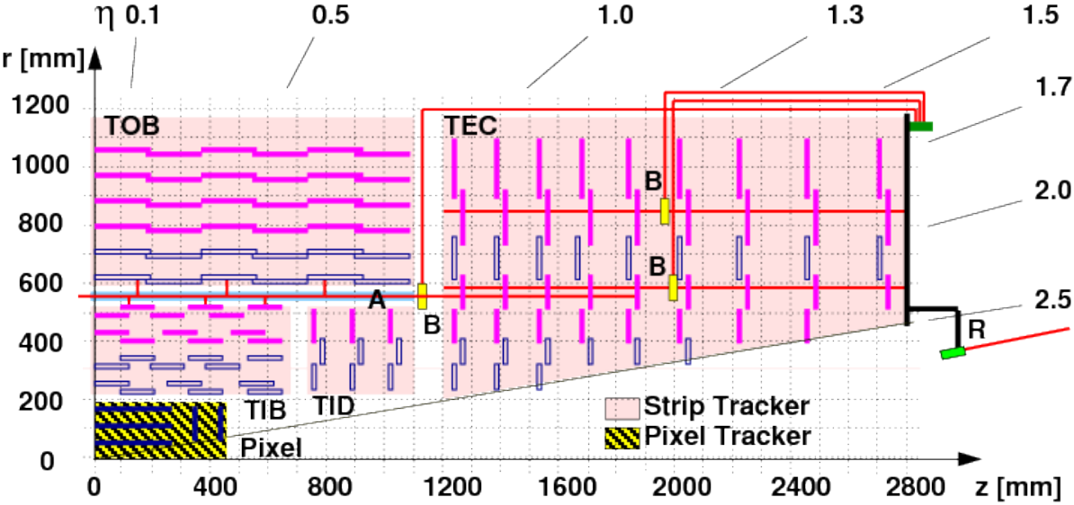
The CMS tracker is composed of 1440 silicon pixel and 15 148 silicon microstrip modules organised in six sub-assemblies, as shown in figure 1. Pixel modules of the CMS tracker are grouped into the barrel pixel (BPIX) and the forward pixel (FPIX) in the endcap regions. Strip modules in the central pseudorapidity region are divided into the tracker inner barrel (TIB) and the tracker outer barrel (TOB) at smaller and larger radii respectively. Similarly, strip modules in the endcap regions are arranged in the tracker inner disks (TID) and tracker endcaps (TEC) at smaller and larger values of -coordinate, respectively.
The BPIX system is divided into two semi-cylindrical half-shells along the - plane. The TIB and TOB are both divided into two half-barrels at positive and negative values, respectively. The pixel modules composing the BPIX half-shells are mechanically assembled in three concentric layers, with radial positions at 4\cm, 7\cm, and 11\cmin the design layout. Similarly, four and six layers of microstrip modules compose the TIB and TOB half-barrels, respectively. The FPIX, TID, and TEC are all divided into two symmetrical parts in the forward () and backward () regions. Each of these halves is composed of a series of disks arranged at different , with the FPIX, TID, and TEC having two, three, and nine such disks, respectively. Each FPIX disk is subdivided into two mechanically independent half-disks. The modules on the TID and TEC disks are further arranged in concentric rings numbered from 1 (innermost) to 3 (outermost) in TID and from 1 up to 7 in TEC.
Pixel modules provide a two-dimensional measurement of the hit position. The pixels composing the modules in BPIX have a rectangular shape, with the narrower side in the direction of the “global” and the larger one along the ”global” -coordinate, where “global” refers to the overall CMS coordinate system introduced at the beginning of this section. Pixel modules in the FPIX have a finer segmentation along global and a coarser one roughly along global , but they are tilted by 20∘ around . Strip modules positioned at a given in the barrel generally measure the global coordinate of the hit. Similarly, strip modules in the endcaps measure the global coordinate of the hit. The two layers of the TIB and TOB at smaller radii, rings 1 and 2 in the TID, and rings 1, 2, and 5 in the TEC are instrumented with pairs of microstrip modules mounted back-to-back, referred to as “” and “stereo” modules, respectively. The strip direction of the stereo modules is tilted by 100\unitmrad relative to that of the modules, which provides a measurement component in the -direction in the barrel and in the -direction in the endcaps. The modules in the TOB and in rings 5–7 of the TEC contain pairs of sensors with strips connected in series.
The strip modules have the possibility to take data in two different configurations, called “peak” and “deconvolution” modes [17, 18]. The peak mode uses directly the signals from the analogue pipeline, which stores the amplified and shaped signals every 25\unitns. In the deconvolution mode, a weighted sum of three consecutive samples is formed, which effectively reduces the rise time and contains the whole signal in 25\unitns. Peak mode is characterised by a better signal-over-noise ratio and a longer integration time, ideal for collecting cosmic ray tracks that appear at random times, but not suitable for the high bunch-crossing frequency of the LHC. Therefore, the strip tracker is operated in deconvolution mode when recording data during the LHC operation. The calibration and time synchronization of the strip modules are optimized for the two operation modes separately.
A local right-handed coordinate system is defined for each module with the origin at the geometric centre of the active area of the module. As illustrated in the left panel of figure 2, the -axis is defined along the more precisely measured coordinate of the module (typically along the azimuthal direction in the global system), the -axis orthogonal to the -axis and in the module plane, pointing away from the readout electronics, and the -axis normal to the module plane. The origin of the -axis is in the middle of the module thickness. For the pixel system, is chosen orthogonal to the magnetic field, \iein the global direction in the BPIX and in the radial direction in the FPIX. The -coordinate is perpendicular to in the sensor plane, \iealong global in the BPIX and at a small angle to the global direction in the FPIX. The angles , , and indicate right-handed rotations about the -, -, and -axes, respectively. As illustrated in the right panel of figure 2, the local track angle () with respect to the module normal is defined in the - (-) plane.
0.3 Global position and orientation of the tracker
While the track based internal alignment (see section 0.4) mainly adjusts the positions and angles of the tracker modules relative to each other, it cannot ascertain the absolute position and orientation of the tracker. Survey measurements of the TOB, as the largest single sub-component, are thus used to determine its shift and rotation around the beam axis relative to the design values. The other sub-components are then aligned relative to the TOB by means of the track based internal alignment procedure. The magnetic field of the CMS solenoid is to good approximation parallel to the -axis. The orientation of the tracker relative to the magnetic field is of special importance, since the correct parameterisation of the trajectory in the reconstruction depends on it. This global orientation is described by the angles and , which correspond to rotations of the whole tracker around the - and -axes defined in the previous section. Uncorrected overall tilts of the tracker relative to the magnetic field could result in biases of the reconstructed parameters of the tracks and the measured masses of resonances inferred from their charged daughter particles. Such biases would be hard to disentangle from the other systematic effects addressed in section 0.4.4. It is therefore essential to determine the global tracker tilt angles prior to the overall alignment correction, because the latter might be affected by a wrong assumption on the magnetic field orientation. It is not expected that tilt angles will change significantly with time, hence one measurement should be sufficient for many years of operation. The tilt angles have been determined with the 2010 CMS data, and they have been used as the input for the internal alignment detailed in subsequent sections of this article. A repetition of the procedure with 2011 data led to compatible results.
The measurement of the tilt angles is based on the study of overall track quality as a function of the and angles. Any non-optimal setting of the tilt angles will result, for example, in incorrect assumptions on the transverse field components relative to the tracker axis. This may degrade the observed track quality. The tilt angles and are scanned in appropriate intervals centred around zero. For each set of values, the standard CMS track fit is applied to the whole set of tracks, and an overall track quality estimator is determined. The track quality is estimated by the total of all the fitted tracks, . As cross-checks, two other track quality estimators are also studied: the mean normalised track per degree of freedom, , and the mean p value, , which is the probability of the to exceed the value obtained in the track fit, assuming a distribution with the appropriate number of degrees of freedom. All methods yield similar results; remaining small differences are attributed to the different relative weight of tracks with varying number of hits and the effect of any remaining outliers.
Events are considered if they have exactly one primary vertex reconstructed by using at least four tracks, and a reconstructed position along the beam line within \unitcm of the nominal centre of the CMS detector. Tracks are required to have at least ten reconstructed hits and a pseudorapidity of . The track impact parameter with respect to the primary vertex must be less than 0.15\unitcm (2\unitcm) in the transverse (longitudinal) direction. For the baseline analysis that provides the central values, the transverse momentum threshold is set to 1\GeVc; alternative values of 0.5 and 2\GeVcare used to check the stability of the results. Only tracks with are selected in order to reject those with wrongly associated hits. For each setting of the tilt angles, each track is refitted by using a full 3D magnetic field model [19, 20] that also takes tangential field components into account. This field model is based on measurements obtained during a dedicated mapping operation with Hall and NMR probes [21].
Each tilt angle is scanned at eleven settings in the range 2\unitmrad. The angle of correct alignment is derived as the point of maximum track quality, corresponding to minimum total , determined by a least squares fit with a second-order polynomial function. The dependence of the total divided by the number of tracks on the tilt angles and is shown in figure 3.
In each plot, only one angle is varied, while the other remains fixed at 0. The second-order polynomial fit describes the functional dependence very well. There is no result for the scan point at \unitmrad, because this setting is outside the range allowed by the track reconstruction programme. While the dependence is symmetric with a maximum near , the dependence is shifted towards positive values, indicating a noticeable vertical downward tilt of the tracker around the -axis with respect to the magnetic field. On an absolute scale, the tilt is small, but nevertheless visible within the resolution of beam line tilt measurements [15].
Figure 4 shows the resulting values of and for five intervals of track pseudorapidity, for tracks with for the total estimator. The statistical uncertainties are taken as the distance corresponding to a one unit increase of the total ; they are at most of the order of the symbol size and thus hardly visible. The outer error bars show the root mean square (RMS) of the changes observed in the tilt angle estimates when changing the track quality estimators and the \ptthreshold. The right plot shows the results of the method applied to simulated events without any tracker misalignment. They are consistent with zero tilt within the systematic uncertainty. The variations are smaller in the central region within , and they are well contained within a margin of 0.1\unitmrad, which is used as a rough estimate of the systematic uncertainty of this method. The left plot in figure 4 shows the result obtained from data; the values are systematically shifted by 0.3\unitmrad, while the values are close to zero. The nominal tilt angle values used as alignment constants are extracted from the central region of figure 4 (left) as \unitmrad and \unitmrad, thus eliminating an important potential source of systematic alignment uncertainty. These results represent an important complementary step to the internal alignment procedure described in the following sections.
0.4 Methodology of track based internal alignment
Track-hit residual distributions are generally broadened if the assumed positions of the silicon modules used in track reconstruction differ from the true positions. Therefore standard alignment algorithms follow the least squares approach and minimise the sum of squares of normalised residuals from many tracks. Assuming the measurements , \ieusually the reconstructed hit positions on the modules, with uncertainties are independent, the minimised objective function is
| (1) |
where is the trajectory prediction of the track model at the position of the measurement, depending on the geometry () and track () parameters. An initial geometry description is usually available from design drawings, survey measurements, or previous alignment results. This can be used to determine approximate track parameters . Since alignment corrections can be assumed to be small, can be linearised around these initial values. Minimising after the linearisation leads to the normal equations of least squares. These can be expressed as a linear equation system with , \iethe alignment parameters and corrections to all parameters of all used tracks . If the alignment corrections are not small, the linear approximation is of limited precision and the procedure has to be iterated.
For the alignment of the CMS tracker a global-fit approach [22] is applied, by using the Millepede II program [23]. It makes use of the special structure of that facilitates, by means of block matrix algebra, the reduction of the large system of equations to a smaller one for the alignment parameters only,
| (2) |
Here and sum contributions from all tracks. To derive , the solutions of the track fit equations are needed. For , also the covariance matrices have to be calculated. The reduction of the matrix size from to is dramatic. For tracks with on average 20 parameters and alignment parameters, the number of matrix elements is reduced by a factor larger than . Nevertheless, no information is lost for the determination of the alignment parameters .
The following subsections explain the track and alignment parameters and that are used for the CMS tracker alignment. Then the concept of a hierarchical and differential alignment by using equality constraints is introduced, followed by a discussion of “weak modes” and how they can be avoided. The section closes with the computing optimisations needed to make Millepede II a fast tool with modest computer memory needs, even for the alignment of the CMS tracker with its unprecedented complexity.
0.4.1 Track parameterisation
In the absence of material effects, five parameters are needed to describe the trajectory of a charged particle in a magnetic field. Traversing material, the particle experiences multiple scattering, mainly due to Coulomb interactions with atomic nuclei. These effects are significant in the CMS tracker, \iethe particle trajectory cannot be well described without taking them into account in the track model. This is achieved in a rigorous and efficient way as explained below in this section, representing an improvement compared to previous Millepede II alignment procedures [10, 11, 13] for the CMS silicon tracker, which ignored correlations induced by multiple scattering.
A rigorous treatment of multiple scattering can be achieved by increasing the number of track parameters to , \egby adding two deflection angles for each of the thin scatterers traversed by the particle. For thin scatterers, the trajectory offsets induced by multiple scattering can be ignored. If a scatterer is thick, it can be approximately treated as two thin scatterers. The distributions of these deflection angles have mean values of zero. Their standard deviations can be estimated by using preliminary knowledge of the particle momentum and of the amount of material crossed. This theoretical knowledge is used to extend the list of measurements, originally containing all the track hits, by “virtual measurements”. Each scattering angle is virtually measured to be zero with an uncertainty corresponding to the respective standard deviation. These virtual measurements compensate for the degrees of freedom introduced in the track model by increasing its number of parameters. For cosmic ray tracks this complete parameterisation often leads to . Since in the general case the effort to calculate is proportional to , a significant amount of computing time would be spent to calculate and thus and . The progressive Kalman filter fit, as used in the CMS track reconstruction, avoids the scaling by a sequential fit procedure, determining five track parameters at each measurement. However, the Kalman filter does not provide the full (singular) covariance matrix of these parameters as needed in a global-fit alignment approach. As shown in [24], the Kalman filter fit procedure can be extended to provide this covariance matrix, but since Millepede II is designed for a simultaneous fit of all measurements, another approach is followed here.
The general broken lines (GBL) track refit [25, 26] that generalises the algorithm described in Ref. [27], avoids the scaling for calculating by defining a custom track parameterisation. The parameters are , where is the change of the inverse momentum multiplied by the particle charge and are the two-dimensional offsets to an initial reference trajectory in local systems at each scatterer and at the first and last measurement. All parameters except influence only a small part of the track trajectory. This locality of all track parameters (but one) results in being a bordered band matrix with band width and border size , \iethe matrix elements are non-zero only for , or . By means of root-free Cholesky decomposition () of the band part into a diagonal matrix and a unit left triangular band matrix , the effort to calculate and is reduced to and , respectively. This approach saves a factor of 6.5 in CPU time for track refitting in Millepede II for isolated muons (see section 0.5) and of 8.4 for cosmic ray tracks in comparison with an (equivalent) linear equation system with a dense matrix solved by inversion.
The implementation of the GBL refit used for the Millepede II alignment of the CMS tracker is based on a seed trajectory derived from the position and direction of the track at its first hit as resulting from the standard Kalman filter track fit. From the first hit, the trajectory is propagated taking into account magnetic-field inhomogeneities, by using the Runge–Kutta technique, and the average energy loss in the material as for muons. As in the CMS Kalman filter track fit, all traversed material is assumed to coincide with the silicon measurement planes that are treated as thin scatterers. The curvilinear frame defined in [28] is chosen for the local coordinate systems at these scatterers. Parameter propagation along the trajectory needed to link the local systems uses Jacobians assuming a locally constant magnetic field between them [28]. To further reduce the computing time, two approximations are used in the standard processing: material assigned to stereo and modules that are mounted together is treated as a single thin scatterer, and the Jacobians are calculated assuming the magnetic field to be parallel to the -axis in the limit of weak deflection, . This leads to a band width of in the matrix .
0.4.2 Alignment parameterisation
To first approximation, the CMS silicon modules are flat planes. Previous alignment approaches in CMS ignored possible deviations from this approximation and determined only corrections to the initial module positions, \ieup to three shifts (, , ) and three rotations (, , ). However, tracks with large angles of incidence relative to the silicon module normal are highly sensitive to the exact positions of the modules along their directions and therefore also to local variations if the modules are not flat. These local variations can arise from possible curvatures of silicon sensors and, for strip modules with two sensors in a chain, from their relative misalignment. In fact, sensor curvatures can be expected because of tensions after mounting or because of single-sided silicon processing as for the strip sensors. The specifications for the construction of the sensors required the deviation from perfect planarity to be less than 100\mum [1]. To take into account such deviations, the vector of alignment parameters is extended to up to nine degrees of freedom per sensor instead of six per module. The sensor shape is parameterised as a sum of products of modified (orthogonal) Legendre polynomials up to the second order where the constant and linear terms are equivalent to the rigid body parameters , and :
| (3) |
Here () is the position on the sensor in the - (-) direction, normalised to its width (length ). The coefficients , and quantify the sagittae of the sensor curvature as illustrated in figure 5.
The CMS track reconstruction algorithm treats the hits under the assumption of a flat module surface. To take into account the determined sensor shapes, the reconstructed hit positions in and (for pixel modules) are corrected by and , respectively. Here the track angle from the sensor normal () is defined in the - (-) plane (figure 2), and the track predictions are used for and .
To linearise the track-model prediction , derivatives with respect to the alignment parameters have to be calculated. If is in the local () direction, denoted as () in the following, the derivatives are
| (4) |
Unlike the parameterisation used in previous CMS alignment procedures [29], the coefficients of the first order polynomials and are used as alignment parameters instead of the angles. This ensures the orthogonality of the sensor surface parameterisation. The in-plane rotation is replaced by with . This has the advantage that all parameters have a length scale and their derivatives have similar numerical size.
The pixel modules provide uncorrelated measurements in both and directions. The strips of the modules in the TIB and TOB are parallel along , so the modules provide measurements only in the direction. For TID and TEC modules, where the strips are not parallel, the hit reconstruction provides highly correlated two-dimensional measurements in and . Their covariance matrix is diagonalised and the corresponding transformation applied to the derivatives and residuals as well. The measurement in the less precise direction, after the diagonalisation, is not used for the alignment.
0.4.3 Hierarchical and differential alignment by using equality constraints
The CMS tracker is built in a hierarchical way from mechanical substructures, \egthree BPIX half-layers form each of the two BPIX half-shells. To treat translations and rotations of these substructures as a whole, six alignment parameters for each of the considered substructures can be introduced. The derivatives of the track prediction with respect to these parameters, , are obtained from the six translational and rotational parameters of the hit sensor by coordinate transformation with the chain rule
| (5) |
where is the Jacobian matrix expressing the effect of translations and rotations of the large structure on the position of the sensor.
These large-substructure parameters are useful in two different cases. If the track sample is too small for the determination of the large number of alignment parameters at module level, the alignment can be restricted to the much smaller set of parameters of these substructures. In addition they can be used in a hierarchical alignment approach, simultaneously with the alignment parameters of the sensors. This has the advantage that coherent misplacements of large structures in directions of the non-sensitive coordinate of strip sensors can be taken into account.
This hierarchical approach introduces redundant degrees of freedom since movements of the large structures can be expressed either by their alignment parameters or by combinations of the parameters of their components. These degrees of freedom are eliminated by using linear equality constraints. In general, such constraints can be formulated as
| (6) |
where the index runs over all the alignment parameters. In Millepede II these constraints are implemented by extending the matrix equation (2) by means of Lagrangian multipliers. In the hierarchical approach, for each parameter of the larger structure one constraint with has to be applied and then all constraints for one large structure form a matrix equation,
| (7) |
where are the shift and rotation parameters of component of the large substructure. Similarly, the technique of equality constraints is used to fix the six undefined overall shifts and rotations of the complete tracker.
The concept of “differential alignment” means that in one alignment step some parameters are treated as time-dependent while the majority of the parameters stays time-independent. Time dependence is achieved by replacing an alignment parameter in the linearised form of equation (1) by several parameters, each to be used for one period of time only. This method allows the use of the full statistical power of the whole dataset for the determination of parameters that are stable with time, without neglecting the time dependence of others. This is especially useful in conjunction with a hierarchical alignment: the parameters of larger structures can vary with time, but the sensors therein are kept stable relative to their large structure.
0.4.4 Weak modes
A major difficulty of track based alignment arises if the matrix in equation (2) is ill-conditioned, \iesingular or numerically close to singular. This can result from linear combinations of the alignment parameters that do not (or only slightly) change the track-hit residuals and thus the overall in equation (1), after linearisation of the track model . These linear combinations are called “weak modes” since the amplitudes of their contributions to the solution are either not determinable or only barely so.
Weak modes can emerge if certain coherent changes of alignment parameters can be compensated by changes of the track parameters . The simplest example is an overall shift of the tracker that would be compensated by changes of the impact parameters of the tracks. For that reason the overall shift has to be fixed by using constraints as mentioned above. Other weak modes discussed below influence especially the transverse momenta of the tracks. A specific problem is that even very small biases in the track model can lead to a significant distortion of the tracker if a linear combination of the alignment parameters is not well determined by the data used in equation (1). As a result, weak modes contribute significantly to the systematic uncertainty of kinematic properties determined from the track fit.
The range of possible weak modes depends largely on the geometry and segmentation of the detector, the topology of the tracks used for alignment, and on the alignment and track parameters. The CMS tracker has a highly segmented detector geometry with a cylindrical layout within a solenoidal magnetic field. If aligned only with tracks passing through the beam line, the characteristic weak modes can be classified in cylindrical coordinates, \ieby module displacements , , and as functions of , , and [30]. To control these weak modes it is crucial to include additional information in equation (1), \egby combining track sets of different topological variety and different physics constraints by means of
- •
cosmic ray tracks that break the cylindrical symmetry,
- •
straight tracks without curvature, recorded when the magnetic field is off,
- •
knowledge about the production vertex of tracks,
- •
knowledge about the invariant mass of a resonance whose decay products are observed as tracks.
Earlier alignment studies [13] have shown that the usage of cosmic ray tracks is quite effective in controlling several classes of weak modes. However, for some types of coherent deformations of the tracker the sensitivity of an alignment based on cosmic ray tracks is limited. A prominent example biasing the track curvature (with being the track charge) is a twist deformation of the tracker, in which the modules are moved coherently in by an amount directly proportional to their longitudinal position (). This has been studied extensively in [31]. Other potential weak modes are the off-centring of the barrel layers and endcap rings (sagitta), described by , and a skew, parameterised as . Here and denote the amplitudes of the sagitta and skew weak modes, whereas and are their azimuthal phases.
As a measure against weak modes that influence the track momenta, such as a twist deformation, information on the mass of a resonance decaying into two charged particles is included in the alignment fit with the following method. A common parameterisation for the two trajectories of the particles produced in the decay is defined as in [32]. Instead of parameters (plus those accounting for multiple scattering), the nine common parameters are the position of the decay vertex, the momentum of the resonance candidate, two angles defining the direction of the decay products in the rest-frame of the resonance, and the mass of the resonance. The mean mass of the resonance is added as a virtual measurement with an uncertainty equal to the standard deviation of its invariant mass distribution. Mean and standard deviation are estimated from the distribution of the invariant mass in simulated decays, calculated from the decay particles after final-state radiation. In the sum on the right hand side of equation (1), the two individual tracks are replaced by the common fit object. With the broken lines parameterisation the corresponding has the border size . This approach to include resonance mass information in the alignment fit implies an implementation of a vertex constraint as well, since the coordinates of the decay vertex are parameters of the combined fit object and thus force the tracks to a common vertex.
The dependence of the reconstructed resonance mass on the size of a twist deformation can be shown to follow
| (8) |
Here denotes the strength of the solenoidal magnetic field along the -axis, () and () are the momentum and its longitudinal component of the positively (negatively) charged particle, respectively. Equation (8) shows that the inclusion of a heavy resonance such as the \Zboson in the alignment procedure is more effective for controlling the twist than the \JPsiand \PgU quarkonia, since at the LHC the decay products of the latter are usually boosted within a narrow cone, and the difference of their longitudinal momenta is small. The decay channel of \Zto muons is particularly useful because the high-\ptmuons are measured precisely and with high efficiency by the CMS detector. The properties of the \Zboson are predicted by the Standard Model and have been characterised experimentally very well at the LHC [33, 34] and in past experiments [35]. This allows the muonic decay of the \Zboson to be used as a standard reference to improve the ability of the alignment procedure to resolve systematic distortions, and to verify the absence of any bias on the track reconstruction.
Under certain conditions, equality constraints can be utilised against a distortion in the starting geometry induced by a weak mode in a previous alignment attempt. The linear combination of the alignment parameters corresponding to the weak mode and the amplitude of the distortion in the starting geometry have to be known. In this case, a constraint used in a further alignment step can remove the distortion, even if the data used in the alignment cannot determine the amplitude. If, for example, each aligned object is, compared to its true position, misplaced in according to a twist with reference point (), this constraint takes the form , where the sums over and include the aligned objects and the sum over includes their active alignment parameters .
0.4.5 Computing optimisation
The Millepede II program proceeds in a two-step approach. First, the standard CMS software environment [5] is used to produce binary files containing the residuals , their dependence on the parameters and of the linearised track model, the uncertainties , and labels identifying the fit parameters. Second, these binary files are read by an experiment-independent program that sets up equation (2), extends it to incorporate the Lagrangian multipliers to implement constraints, and solves it, \egby the iterative Minres algorithm [36]. In contrast to other fast algorithms for solving large matrix equations, Minres does not require a positive definite matrix, and because of the Lagrangian multipliers is indefinite. Since the convergence speed of Minres depends on the eigenvalue spectrum of the matrix , preconditioning is used by multiplying equation (2) by the inverse of the diagonal of the matrix. The elements of the symmetric matrix in general require storage in double precision while they are summed. For the 200 000 alignment parameters used in this study, this would require 160\unitGB of RAM. Although the matrix is rather sparse and only non-zero elements are stored, the reduction is not sufficient. High alignment precision also requires the use of many millions of tracks of different topologies that are fitted several times within Millepede II, leading to a significant contribution to the CPU time. To cope with the needs of the CMS tracker alignment described in this article, the Millepede II program has been further developed, in particular to reduce the computer memory needs, to enlarge the number of alignment parameters beyond what was used in [13], and to reduce the processing time. Details are described in the following.
Since the non-zero matrix elements are usually close to each other in the matrix, further reduction of memory needs is reached by bit-packed addressing of non-zero blocks in a row. In addition, some matrix elements sum contributions of only a few tracks, \egcosmic ray tracks from rare directions. For these elements, single precision storage is sufficient.
Processing time is highly reduced in Millepede II by shared-memory parallelisation by means of the Open Multi-Processing (OpenMP) package [37] for the most computing intensive parts like the product of the huge matrix with a vector for Minres, the track fits for the calculation of and , and the construction of from those. Furthermore, bordered band matrices are automatically detected and root-free Cholesky decomposition is applied subsequently (see section 0.4.1).
Reading data from local disk and memory access are further potential bottlenecks. The band structure of that is due to the GBL refit and the approximations in the track model (see section 0.4.1) also aim to alleviate the binary file size. To further reduce the time needed for reading, Millepede II reads compressed input and caches the information of many tracks to reduce the number of disk accesses.
0.5 Strategy of the internal alignment of the CMS tracker
In general, the tracker has been sufficiently stable throughout 2011 to treat alignment parameters as constant in time. The stability of large structures has been checked as described in section 0.6. An exception to this stability is the pixel detector whose movements have been carefully monitored and are then treated as described below. Validating the statistical alignment precision by means of the methods of section 0.7 shows no need to have a further time dependent alignment at the single module parameter level. Also, calibration parameters influence the reconstructed position of a hit on a module. These parameters account for the Lorentz drift of the charge carriers in the silicon due to the magnetic field and for the inefficient collection of charge generated near the back-plane of strip sensors if these are operated in deconvolution mode. Nevertheless, for 2011 data there is no need to integrate the determination of calibration parameters into the alignment procedure. The hit position effect of any Lorentz drift miscalibration is compensated by the alignment corrections and as long as the Lorentz drift is stable with time, the exact miscalibration has no influence on the statistical alignment precision. Also the back-plane correction has only a very minor influence. No significant degradation of the statistical alignment precision with time has been observed.
Given this stability, the 2011 alignment strategy of the CMS tracker consists of two steps; both apply the techniques and tools described in section 0.4. The first step uses data collected in 2011 up to the end of June, corresponding to an integrated luminosity of about 1\fbinv. This step is based on the full exploitation of different track topologies, making use of resonance mass and vertex information. The details are described in the rest of this section. The second step treats the four relevant movements of the pixel detector after the end of June, identified with the methods of section 0.6.2. Six alignment parameters for each BPIX layer and FPIX half-disk are redetermined by a stand-alone alignment procedure, keeping their internal structures unchanged and the positions of the strip modules constant.
Tracks from several data sets are used simultaneously in the alignment procedure. The following selection criteria are applied:
- •
Isolated muons: Global muons [16] are reconstructed in both the tracker and the muon system. They are selected if their number of hits in the tracker exceeds nine (at least one of which is in the pixel detector, ), their momenta are above 8\GeVc(in order to minimise the effects of Multiple Coulomb scattering), and their transverse momenta \ptare above 5\GeVc. Their distances from the axes of jets reconstructed in the calorimeter and fulfilling have to be larger than 0.1. This class of events is populated mainly by muons belonging to leptonic -boson decays and about 15 million of these tracks are used for the alignment.
- •
Tracks from minimum bias events: a minimum bias data sample is selected online with a combination of triggers varying with pileup conditions, i.e. the mean number of additional collisions, overlapping to the primary one, within the same bunch crossing (on average 9.5 for the whole 2011 data sample). These triggers are based, for example, on pick-up signals indicating the crossing of two filled proton bunches, signals from the Beam Scintillator Counters [1], or moderate requirements on hit and track multiplicity in the pixel detectors. The offline track selection requires , . Three million of these tracks are used for alignment.
- •
Muons from \Z-boson decays: events passing any trigger filter requesting two muons reconstructed online are used for reconstructing \Z-boson candidates. Two muons with opposite charge must be identified as global muons and fulfil the requirement ( ). Their transverse momenta must exceed and their distances to jets reconstructed in the calorimeter . The invariant mass of the reconstructed dimuon system must lie in the range , in order to obtain a pure sample of \Z-boson candidates. The total number of such muon pairs is 375 000.
- •
cosmic ray tracks: cosmic ray events used in the alignment were recorded with the strip tracker operated both in peak and deconvolution modes. Data in peak mode were recorded in a dedicated cosmic data taking period before the restart of the LHC operations in 2011 and during the beam-free times between successive LHC fills. In addition, cosmic ray data were taken in deconvolution mode both during and between LHC fills, making use of a dedicated trigger selecting cosmic ray tracks passing through the tracker barrel. In total 3.6 million cosmic ray tracks with and are used, where about half of the sample has been collected with the strip tracker operating in peak mode, while the other half during operations in deconvolution mode.
For all the data sets, basic quality criteria are applied on the hits used in the track fit and on the tracks themselves:
- •
the signal-over-noise ratio of the strip hits must be higher than 12 (18) when the strip tracker records data in deconvolution (peak) mode;
- •
for pixel hits, the probability of the hit to match the expected shape of the charge cluster for the given track parameters [38] must be higher than () in the () direction;
- •
for all hits, the angle between the track and the module surface must be larger than () for tracks from proton-proton collisions (cosmic rays) to avoid a region where the estimates of the hit position and uncertainty are less reliable;
- •
to ensure a reliable determination of the polar track angle, , tracks have to have at least two hits in pixel or stereo strip modules;
- •
tracks from proton-proton collisions have to satisfy the “high-purity” criteria [14] of the CMS track reconstruction code;
- •
in the final track fit within Millepede II, tracks are rejected if their value is larger than the 99.87% quantile (corresponding to three standard deviations) of the distribution for the number of degrees of freedom of the track.
The tracker geometry, as determined by the alignment with the 2010 data [31], is the starting point of the 2011 alignment procedure. In general, for each sensor all nine parameters are included in the alignment procedure. Exceptions are the coordinate for strip sensors since it is orthogonal to the measurement direction, and the surface parameterisation parameters , , , , for the FPIX modules. The latter exception is due to their small size and smaller sensitivity compared to the other subdetectors, caused by the smaller spread of track angles with respect to the module surface.
The hierarchical alignment approach discussed in section 0.4.3 is utilised by introducing parameters for shifts and rotations of half-barrels and end-caps of the strip tracker and of the BPIX layers and FPIX half-disks. For the parameters of the BPIX layers and FPIX half-disks the differential alignment is used as well. The need for nine time periods (including one for the cosmic ray data before the LHC start) has been identified with the validation procedure of section 0.6.2. The parameters for the six degrees of freedom of each of the two TOB half-barrels are constrained to have opposite sign, fixing the overall reference system.
Three approaches have been investigated to overcome the twist weak mode introduced in section 0.4.4. The first uses tracks from cosmic rays, recorded in 2010 when the magnetic field was off. This successfully controls the twist, but no equivalent data were available in 2011. Second, the twist has been measured in the starting geometry with the method of section 0.9.2. An equality constraint has been introduced to compensate for it. While this method controls the twist, it does not reduce the dependence of the muon kinematics on the azimuthal angle seen in sections 0.9.1 and 0.9.2. Therefore the final alignment strategy is based on the muons from \Z-boson decays to include mass information and vertex constraints in the alignment procedure as described in section 0.4.4, with a virtual mass measurement of .
In total, more than 200 000 alignment parameters are determined in the common fit, by using 138 constraints. To perform this fit, 246 parallel jobs produce the compressed input files containing residuals, uncertainties, and derivatives for the linearised track model for the Millepede II program. The total size of these files is 46.5\unitGB. The matrix constructed from this by Millepede II contains 31% non-zero off-diagonal elements. With a compression ratio of 40% this fits well into an affordable 32\unitGB of memory. The Minres algorithm has been run four times with increasingly tighter rejection of bad tracks. Since is not significantly changed by this rejection, it does not need to be recalculated after the first iteration. By means of eight threads on an Intel Xeon L5520 processor with 2.27\unitGHz, the CPU usage was 44:30\unith with a wall clock time of only 9:50\unith. This procedure has been repeated four times to treat effects from non-linearity: iterating the procedure is particularly important for eliminating the twist weak mode.
The same alignment procedure as used on real data was run on a sample of simulated tracks, prepared with the same admixture of track samples as in the recorded data. The geometry obtained in this way is characterised by a physics performance comparable to the one obtained with recorded data and can be used for comparisons with simulated events. This geometry is referred as the “realistic” misalignment scenario.
0.6 Monitoring of the large structures
A substantial fraction of the analyses in CMS use data reconstructed immediately after its acquisition (prompt reconstruction) for obtaining preliminary sets of results. Therefore, it is important to provide to the physics analyses the best possible geometry for use in the prompt reconstruction, immediately correcting any possible time-dependent large misalignment. Specifically, the position of the large structures in the pixel detector is relevant for the performance of b-tagging algorithms. As described in [8], misalignment at the level of a few tens of microns can seriously affect the b-tagging performance.
In order to obtain the best possible track reconstruction performance, the tracker geometry is carefully monitored as a function of time, so that corrections can be applied upon movements large enough to affect the reconstruction significantly. The CMS software and reconstruction framework accommodates time-dependent alignment and calibration conditions by “intervals of validity” (IOV), which are periods during which a specific set of constants retain the same values [5]. While the alignment at the level of the single modules needs data accumulated over substantial periods of time, the stability of the position of the large structures can be controlled with relatively small amounts of data or via a system of infrared lasers. The short data acquisition times required by these monitoring methods allow fast and frequent feedback to the alignment procedure. A system of laser beams is able to monitor the positions of a restricted number of modules in the silicon strip tracker. Movements of large structures in the pixel tracker can be detected with high precision with collision tracks by a statistical study of the primary-vertex residuals, defined as the distance between the tracks and the primary vertex at the point of closest approach of the tracks to the vertex. All these techniques allow the monitoring of the position of the large structures on a daily basis. This frequent monitoring, together with the fast turn-around of the alignment with Millepede II, allows, if needed, the correction of large movements on the timescale of one day.
0.6.1 Monitoring of the strip tracker geometry
The CMS laser alignment system (LAS) [39] provides a source of alignment information independent of tracks. It is based on 40 near-infrared (1075\unitnm) laser beams passing through a subset of the silicon sensors that are used also for the standard track reconstruction (see figure 1). The laser optics are mounted on mechanical structures independent of those used to support the tracker. With this limited number of laser beams one can align large-scale structures such as the TOB, TIB, and both TECs. The mechanical accuracy of LAS components limits the absolute precision of this alignment method to 50\mumin comparison to the alignment with tracks, which reaches better than 10\mumresolution (see section 0.7), but the response time of the LAS is at the level of only a few minutes. Within this margin of accuracy, the LAS measurement demonstrated very good stability of the strip detector geometry over the whole 2011 running period. This observation is confirmed by a dedicated set of alignments with tracks, where the dataset was divided into different time periods. No significant movements of the large structures of the silicon strip tracker were found.
0.6.2 Monitoring of the pixel detector geometry with tracks
The large number of tracks produced in a pp collision allows precise reconstruction of the interaction vertices [15]. The resolution of the reconstructed vertex position is driven by the pixel detector since it is the sub-structure that is closest to the interaction point and has the best hit resolution. The primary vertex residual method is based on the study the distance between the track and the vertex, the latter reconstructed without the track under scrutiny (unbiased track-vertex residual). Events used in this analysis are selected online with minimum bias triggers as mentioned in section 0.5. The analysis uses only vertices with distances from the nominal interaction point \unitcm and \unitcm in the transverse and longitudinal direction, respectively. The fit of the vertex must have at least 4 degrees of freedom. For each of these vertices, the impact parameters are measured for tracks with:
- •
more than six hits in the tracker, of which at least two are in the pixel detector,
- •
at least one hit in the first layer of the BPIX or the first disk of the FPIX,
- •
,
- •
of the track smaller than 5.
The vertex position is recalculated excluding the track under scrutiny from the track collection. A deterministic annealing clustering algorithm [40] is used in order to make the method robust against pileup, as in the default reconstruction sequence.
The distributions of the unbiased track-vertex residuals in the transverse plane, , and in the longitudinal direction, , are studied in bins of and of the track. Random misalignments of the modules affect only the resolution of the unbiased track-vertex residual, increasing the width of the distributions, but without biasing their mean. Systematic movements of the modules will bias the distributions in a way that depends on the nature and size of the misalignment and the and of the selected tracks. As an example, the dependence of the means of the and distributions as a function of the azimuthal angle of the track is shown in figure 6. The focus on the -dependence is motivated by the design of the BPIX, which is divided into one half-shell with modules at and another with modules at . Small movements of the two half-shells are mechanically allowed by the mechanical design of the pixel detector. The observed movements have not been associated to a specific cause, although thermal cycles executed on the pixel detector increase the chances that such movements will happen. As an example, the impact of a movement of one half-shell with respect to the other in the longitudinal direction is shown by the open circles in figure 6 for a simulated sample of minimum bias events. Such a movement is reflected in a very distinctive feature in the dependence of the mean of the distribution as a function of . The size of the movement can be estimated as the average bias in the two halves of the BPIX. The time dependence of this quantity in the 2011 data is illustrated in figure 7, which shows some discontinuities. Studies carried out on simulated data show that the b-tagging performance is visibly degraded in the case of uncorrected shifts with amplitude [8]. For this reason, IOVs with different alignments of the pixel layers are conservatively defined according to the boundaries of periods with steps of larger than 10\mum. The time-dependent alignment parameters of BPIX layers and FPIX half-disks during the first eight IOVs (until end of June 2011) were determined in a single global fit. Within each time interval, the positions of the modules with respect to the structure were found not to need any further correction. Because of this, the positions of the pixel layers and half-disks were determined by a dedicated alignment procedure keeping the other hierarchies of the geometry unchanged. The aligned geometry performs well over the entire data-taking period, reducing the observed jumps in the expected way. Residual variations can be attributed to small misalignments with negligible impact on physics performance and to the resolution of the validation method itself.
0.7 Statistical accuracy of the alignment
A method for assessing the achieved statistical precision of the aligned positions in the sensitive direction of the modules has been successfully explored and adopted in the alignment of the CMS tracker during commissioning with cosmic rays, described in [13]. The results from the validation are based on isolated muon tracks with a transverse momentum of \GeVcand at least ten hits in the tracker. The tracks are refitted with the alignment constants under study. Hit residuals are determined with respect to the track prediction, which is obtained without using the hit in question to avoid any correlation between hit and track. From the distribution of the unbiased hit residuals in each module, the median is taken and histogrammed for all modules in a detector subsystem. The median is relatively robust against stochastic effects from multiple scattering, and thus the distribution of the medians of residuals (DMR) is a measure of the alignment accuracy. Only modules with at least 30 entries in their distribution of residuals are considered.
The addition of proton-proton collision events leads to a huge increase of the number of tracks available for the alignment, especially for the innermost parts of the tracker. Compared to the alignment with cosmic rays alone [13], considerable improvements are consequently observed in the pixel tracker, especially in the endcaps. The corresponding DMR are shown in the figure 8, separately for the and coordinates; for both pixel tracker barrel (BPIX) and endcap (FPIX) detectors, the RMS is well below 3\mumin both directions, compared to about 13\mumfor the endcaps in the cosmic ray-only alignment. These numbers are identical or at most only slightly larger than those obtained in simulation without any misalignment, which are below 2\mumand thus far below the expected hit resolution. In the case of no misalignment, the remaining DMR width is non-zero because of statistical fluctuations reflecting the limited size of the track sample. Thus, the DMR width of the no-misalignment case indicates the intrinsic residual uncertainty of the DMR method itself. The remaining uncertainty after alignment determined from recorded data is close to the sensitivity limit of the DMR method. The DMR obtained with the realistic misalignment scenario (see section 0.5) are also shown in figure 8. The distributions are very close to the ideal case.
The alignment accuracy of the strip detector is investigated in smaller groups of sensors with a different method by using normalised residuals [41]. Each group consists of sensors that are expected to have similar alignment accuracy. The distinction is by layer (“L”) or ring (“R”) number, by longitudinal hemisphere (“” and “” for positive and negative coordinate, respectively), and according to whether the surface of a barrel module points inwards (“i”), \ietowards the beamline, or outwards (“o”). The letter “S” indicates a stereo module. The method applied here is based on the widths of the distributions of normalised unbiased residuals of each sensor group. Since the misalignment dilutes the apparent hit resolution, its degree can be derived from the widening of these distributions of normalised residuals. The residual resolution is the square root of the quadratic sum of the resolutions of the intrinsic hit reconstruction and of the track prediction, excluding the hit in question. The alignment uncertainty is added in quadrature to the intrinsic hit resolution of the cluster and adjusted such that the width of the distribution of normalised residuals matches the ideal one, which is determined from simulated events. In this way, misalignment in all degrees of freedom of the modules is contributing to the measurement.
Since the width of each distribution of normalised residuals is also influenced by the alignment uncertainties of the surrounding detector areas, these parameters are highly coupled, and iteration is required. Each track is refitted with the current estimate of all alignment uncertainties taken into account, and the procedure is repeated. In each iteration, a damping factor of 0.6 is applied to the correction to mitigate oscillations. Convergence is achieved after 15 iterations.
The resulting alignment accuracy per sensor group, , is shown in figure 9 for the TIB, TID and TEC subsystems. In all cases, a significant improvement resulting from the alignment procedure is observed. The alignment accuracy is between 3–8\mumfor TIB, between 6–10\mumfor TID, and better than 13\mumfor the TEC. The only exception in ring 7 of the TEC is well understood; it is due to a systematic misplacement of these sensors in the (almost insensitive) radial direction by about 1.3\mm, which has been corrected for in further alignment procedures. For large parts of the TOB and the pixel detector, the remaining misalignment cannot be distinguished from zero within the systematic limitations of this method.
Overall, the statistical accuracy of the alignment is such that its effect is small compared to the intrinsic measurement precision of the sensors. It should be noted, however, that quality estimators based on track-residual distributions have little or no sensitivity to weak modes; these will be addressed in section 0.9.
0.8 Sensor and module shape parameters
As discussed in section 0.4.2, the tracker modules are not expected to be absolutely flat. If a silicon module is not flat, the local -coordinate of the point where a track intersects the sensor (see figure 2) depends on the relative position (, ). The module shape can thus be investigated by track-hit residuals in as a function of the track position on the module [30]. These residuals can be calculated from the one in the -direction and the track angle (figure 2), The mean values of these residuals are shown in figures 10 and 11 as a function of the relative local track coordinates and , averaged over many modules of the strip and pixel subdetectors, respectively. Since tracks with a large angle relative to the surface normal are most sensitive to any deviation from flatness, each residual in the average is weighted by .
Several module shape parameterisations are investigated in the alignment procedure as shown in figures 10 and 11. The blue open circles are deduced by using alignment constants obtained in a procedure similar to the one described in section 0.5, but without taking any module shape parameters into account. Clear deviations from zero are observed in almost all cases, indicating that the modules are systematically not flat. The red filled triangles are obtained with the same alignment procedure except that the two sensors of the modules in the TOB and in the TEC rings 5–7 are aligned independently. Finally, the black points represent the full alignment.
For the distributions along for “flat modules”, a parabolic shape of the sensors of all subdetectors is clearly observed. These structures are correctly compensated when curvatures are taken into account as for the “curved sensors”. At the largest values of in the TEC there are few tracks since the modules are wedge-like in shape and their widths are defined by their longer edges. The distributions along the strip direction () show more varied features. In the TIB, a structure remains that could be corrected by a fourth order polynomial, but the amplitude is only a few and thus negligible for tracking purposes. For the TOB, the V-shaped curve of the “flat modules” parameterisation indicates a systematic kink between the two sensors of the modules. After correcting for the relative misalignment of the sensors by means of the “flat sensors” parameterisation, a parabolic shape can be seen for the sensors at positive . Only the use of the “curved sensors” correction results in a flat dependence. For the double-sensor modules in the TEC rings 5–7, no systematic kink between the sensors is visible. However, both sensors are clearly curved, which is corrected for with the “curved sensors” parameterisation.
In the pixel detectors, no systematic structure is observed along the -direction. The mean -residual distributions along the -direction, determined with tracks from proton-proton collisions, is shown in figure 11.
An average curvature of the BPIX modules can clearly be seen. The FPIX modules also show curvatures, but with smaller amplitude. No corrections are necessary for this subtle effect.
The “curved sensor” parameterisation leads to a sizable improvement of the quality of the tracks that cross modules with large angles relative to the module normal; specifically, cosmic ray tracks crossing the barrel of the tracker from the top to the bottom with large distances of closest approach to the beam line predominantly have these large track angles. Figure 12 shows the average fit probability as a function of for cosmic ray tracks.
Tracks with small cross the modules with modest angles relative to the normal. With larger , the average angle of incidence of the track with respect to the module also increases, resulting in a significant degradation of the average fit quality for the “flat modules” parameterisation. For “curved sensors” the distribution is approximately flat for \cm, resulting in improved consistency of the important cosmic ray track sample with tracks from proton-proton collisions. The remaining features of the dependence are correlated with the radii of the barrel layers. If tracks cross a layer tangentially, the treatment of multiple scattering effects by using thin scatterers only is an oversimplified approximation.
The average sizes of the sagittae of the sensor curvatures along the - () and -direction (), as determined sensor-by-sensor, are shown in figure 13 for the different layers and rings, further differentiating for stereo and modules, \iegrouping modules with similar sensors and mounting.
While the average sagitta for BPIX sensors is almost zero, it is usually around in the strip subdetectors. This matches well the sagittae of the average module shapes along seen for the “flat module” distributions on the left pane of figure 10. Stronger curvatures with average sagittae up to are observed for specific sensor types and mounting positions, \egthe modules in TEC ring 2. The average sagitta shows variations from for BPIX modules (matching with the left pane of figure 11) to almost \mumfor some sensor types in the TEC. While the average sensor sagittae shown here are clearly below the construction specifications of 100\mum, the tails of the distributions extend to \mumand even beyond. This could be due to stresses induced by the mechanics.
Aligning both sensors of the modules in the TOB and the TEC rings 5–7 independently indicates that the sensors were slightly misaligned with respect to each other during module assembly. As an example, figure 15 shows their average differences of the rotation angles around the local -axis, , where the first sensor is the one closer to the readout electronics at .
The TOB modules show an average kink of \unitmrad, matching well the kink seen in the TOB graph \vs of figure 10. The value varies significantly among different modules in the TEC. This variation has averaged out the kink effect in the TEC distribution \vs. The angular misalignment of the two sensors exhibits a significant spread as shown for and, for the rotation around , of the TOB modules in figure 15. Values of \unitmrad are reached, corresponding to at the edges of the 10\cmlong sensors.
In summary, the module shapes can be described with polynomials up to the second order for each sensor, and their coefficients are successfully determined sensor-by-sensor within the alignment procedure. Applying corrections to the hit positions that depend on the module parameters determined and on the track parameters on the module surface significantly improves the overall track description, especially for the important cosmic ray tracks. The sensor parameterisation used here is valid as long as the effect of the curvatures can be approximated by a change of the local coordinate only, neglecting changes in and . Within these boundaries, the construction criterion of sensor bows below 100\mumcould have been relaxed since the alignment successfully takes care of this effect.
0.9 Control of systematic misalignment
The monitoring of standard physics references and the comparison with other subdetectors of CMS provides a direct check of the robustness of the alignment procedure and potentially indicates the presence of systematic misalignments. This information can be included in the alignment algorithm in order to better constrain the systematic misalignments, as described in section 0.4.4. The sensitivity to weak modes of the alignment procedure followed in this analysis is discussed in section 0.9.3 following the approach presented in [13, 30].
0.9.1 Monitoring of the tracker geometry with events
As described in sections 0.4.4 and 0.5, muonic decays of \Zbosons provide a standard reference that can be used for validating the aligned geometry. The selection of well-reconstructed candidates requires two muons reconstructed with both the tracker and the muon system (global muons), where at least one of them passes the tight quality selections as defined in [16]. The muons must pass the following kinematic selections:
- •
\GeVc,
- •
,
- •
\GeVcc.
The distribution of the mass of the \Zcandidates is then fitted with a Voigtian function to model the reconstructed \Z-boson lineshape and an exponential function to model the background. The width of the Breit–Wigner component of the Voigtian function is fixed to the decay width of the \Zboson. The mass of the \Zcandidates is estimated with the mean of the fitted Voigtian. The reconstructed mass is slightly below the nominal mass of 91.2\GeVcc, at about 90.8\GeVcc, mostly because of the presence of QED final-state radiation [16]. The mass of the \Zcandidates is measured as a function of and of the positively charged muon. A twist-like weak mode would bias the curvature measurement of each muon depending on its polar angle, manifesting itself as a strong dependence of the \Z-boson mass on the muon pseudorapidity (with opposite signs for the two muon charges).
The result of this study is presented in figure 16 for both the 2011 data and the simulation, and the corresponding dependence of the \Z-boson mass on the difference in pseudorapidity of the two muons, , is shown in figure 17. By using the nominal geometry, the estimated value of the \Z-boson mass in the simulation is 90.8\GeVcc, as expected after final-state radiation. Without using the \Z-boson mass information (downward-pointing triangles), a pronounced and dependence of the reconstructed invariant mass is observed, which extends over a range of more than 5\GeVccand is attributed to a twist weak mode as seen in section 0.9.2. The inclusion of the \Z-boson mass information (upward-pointing triangles) removes this bias and leads to an almost flat dependence on and .
The agreement between the data and the simulation is good. A small offset of about 100\MeVccin the simulation with respect to the data is visible. The size of any remaining bias, also as a function of the azimuthal angle, is of the order of a few per mil and thus small compared to the \ptresolution targeted for muons in the typical momentum range of the \Z-boson decays, which is at best 1% [16]. This suggests that in terms of performance the aligned geometry in data is very close to a perfectly aligned tracker, with a beneficial impact on the physics measurements of CMS. Offline corrections to the muon momentum can be applied after the reconstruction level, further improving the momentum scale and resolution of the muons [16].
0.9.2 Monitoring of the tracker geometry with the CMS calorimeter
The measurements of the CMS electromagnetic and hadron calorimeters can be exploited to study systematic effects in the momentum measurement. This check is valuable since it is an alternative to the decays, which are already used in the alignment procedure. Weak modes altering the true azimuthal angle of the modules would modify the track curvature in the opposite way for positively and negatively charged tracks. If denotes the change of the azimuthal position at the radius of a track due to bending in the magnetic field, the following relation holds for the reconstructed \ptof the track in case of a twist-like deformation:
| (9) |
A longitudinal magnetic field strength of 3.8 T is assumed. The indicates the electric charge of the particle, is the radius (measured in metres) at which the particle leaves the tracker volume, and is the azimuthal misplacement of the hits due to the deformation. So the relative angle is related to the asymmetry in the \ptmeasurement of oppositely charged tracks with the same true \ptand same . An external measurement of the energy of the charged particle, , is provided by the ECAL and the HCAL [42]. At a given value of , the average ratio between the energy and momentum of a charged track at fixed \pt, is measured as a function of the asymmetry between positively and negatively charged tracks, :
| (10) |
which for large \pt() and small misalignments () approximates to
| (11) |
The track sample used for the validation is selected from an input data set of events triggered by requiring a track with a total momentum and matched to an HCAL cluster. A charged-track isolation requirement is applied at the trigger level ensuring that no track with a transverse momentum of is allowed to be in a circle with a radius of 40\cmaround the impact point on the ECAL surface of the track considered. The distributions of and for particles with similar energy are fitted with a Gaussian function. The means of the fits are used in equation (11) in order to measure the for that specific bin. The results for different bins of the calorimeter energy are finally averaged. This method uses the calorimetric information only to identify tracks with the same energy, improving its robustness against miscalibrations of the absolute energy scale of the calorimeters. The dependence of on the -component of the impact point at the radial position \unitm and on the of the track is shown in figure 18 for different geometries. A twist deformation would show as a linear trend in the dependence. From the observed dependence, no significant systematic distortion in the aligned geometry is visible within the current uncertainties of the validation method. A clear improvement with respect to a geometry not exploiting the mass information is visible. A linear fit to the distributions is performed in order to quantify the bias. In the absence of the mass information in the alignment procedure, the linear fit exhibits a slope significantly different from zero, . In the case of the baseline alignment on data, the slope is . Slopes compatible with zero are observed also in the simulation case, both without misalignment and in the realistic misalignment scenario. A layer rotation, \iea systematic rotation of the layers with an amplitude proportional to the radius (), would appear as a constant offset. The -dependence displays the same trend as already seen in the validation with decays of figure 16. The trend of is quantitatively characterised by means of a fit to the binned distribution with a sinusoidal function. The fit returns a parameterisation of .
0.9.3 Sensitivity to systematic misalignment
Beyond the validation of the aligned geometry, the sensitivity to weak modes of the alignment procedure has been studied. Following the approach in [13, 30], a set of basic deformations were applied on top of the aligned tracker geometry. The full alignment procedure was then repeated starting from the misaligned scenario, obtaining a set of ”realigned” geometries. Nine systematic misalignment scenarios were studied, giving a matrix of deformations expressed with , , and as a function of the same three variables. These misalignments were applied only to the directions to which the silicon modules are effectively sensitive. Movements along non-measurement directions (\egthe longitudinal direction for strip barrel modules) are irrelevant, since the alignment procedure does not associate any parameters with them.
The ability of the alignment procedure to compensate for misalignments indicates its robustness against systematic distortions of this or similar type. A close match between the realigned and initial geometry means that the procedure is fully sensitive to this specific deformation and able to keep it under control. On the other hand, few or no changes compared to the misaligned scenario indicate poor sensitivity.
The left-hand side of figure 19 displays the difference between the positions of the modules in the initial aligned and the deliberately misaligned geometry for some benchmark misalignment scenarios. The behaviour of the distribution of the normalised for the three stages of the study (initially aligned, misaligned and realigned) is presented in the right-hand side of figure 19, by using a sample of isolated muons. The upper, middle and bottom rows present the cases of twist, skew and sagitta deformations as introduced in section 0.4.4. The results show that the alignment procedure has very good control over twist-like deformations. The normalised of the isolated muons does not change significantly when introducing the twist-like deformation because this type of tracks does not have sensitivity to it. The control over twists comes largely from the constraining power of the muonic \Z-boson decays. Skew and sagitta are interesting because they are the systematic distortions most difficult to control. The skew misalignment is fully recovered in the pixel barrel, but not in the other subdetectors. The alignment procedure is only partially resilient against sagitta distortion, with the best recovery observed at small radii. The other six misalignment scenarios considered prove to be well controlled. These results represent a significant improvement with respect to [13], thanks to the inclusion of tracks from proton-proton collisions with several different topologies and the usage of vertex constraint and mass information with muons coming from \Z-boson decays.
0.10 Summary
The alignment procedure for the CMS tracker and its results for the first high-luminosity data-taking period during the year 2011 have been presented. Among the most prominent features are the successful handling of the large degree of complexity of a highly granular silicon detector, the simultaneous determination of shape parameters at the sensor level, the use of the Z resonance signature to control systematic effects, and the parallelised implementation of the whole procedure resulting in a fast execution of the workflow.
The alignment is based on global minimisation of track-to-hit residuals. The internal alignment is performed with the Millepede II algorithm, which is enhanced compared to its predecessor to handle about 200 000 alignment parameters simultaneously. A dedicated track parameterisation is included, based on the general broken lines method, which allows rigorous and execution-time-efficient treatment of multiple scattering in the global fit. The execution time of the fit is considerably shortened by parallelisation on a multi-core architecture.
The time dependence of the tracker alignment is monitored with laser beams and tracks. The tracker geometry is found to be very stable with time. The most important movements are observed between the half-shells of the barrel pixel detector, whose longitudinal separation varies by up to 40\mum. The alignment procedure corrects for these movements such that the residual variation after alignment is kept below 10\mum.
The overall tilt angles of the tracker with respect to the magnetic field are determined to be at the sub-mrad level. The statistical accuracy of the alignment is found to be generally—often significantly—better than 10\mum, with the exception of some rings in the tracker endcap disks. Sensor- and module-shape parameters are determined at the module level simultaneously with other alignment parameters. Curvatures of individual sensors and kink angles of adjacent sensors in modules are observed and measured; sensor curvature amplitudes vary according to subsystem, and their averages per layer and ring range up to about 80\mumin the endcap systems. Kink angles of up to several mrad are observed.
Besides cosmic ray tracks, reconstructed decays play an essential role in constraining systematic deformations of the aligned geometry with small leverage to the track , also known as weak modes. The remaining variation of the \Z-boson mass peak is less than 0.5% and thus small compared to other resolution effects in the corresponding momentum range. The successful control of weak modes is confirmed by studies involving the energy measured in the hadronic calorimeter.
The stability of the alignment with respect to weak modes is further investigated by the study of the effect of deliberately added distortions and subsequent re-alignment. The procedure is found to have very good control over twist modes, while strong sagitta and skew misalignments are at least partially recovered.
In summary, this article describes the comprehensive alignment procedure for the largest and most complex silicon detector ever built. The achieved alignment accuracy enables the tracking to take full benefit of the high intrinsic resolution of the silicon modules. The quality of the alignment is thus an essential building block for the excellent physics performance of the CMS detector.
Acknowledgements
We congratulate our colleagues in the CERN accelerator departments for the excellent performance of the LHC and thank the technical and administrative staffs at CERN and at other CMS institutes for their contributions to the success of the CMS effort. In addition, we gratefully acknowledge the computing centres and personnel of the Worldwide LHC Computing Grid for delivering so effectively the computing infrastructure essential to our analyses. Finally, we acknowledge the enduring support for the construction and operation of the LHC and the CMS detector provided by the following funding agencies: the Austrian Federal Ministry of Science and Research and the Austrian Science Fund; the Belgian Fonds de la Recherche Scientifique, and Fonds voor Wetenschappelijk Onderzoek; the Brazilian Funding Agencies (CNPq, CAPES, FAPERJ, and FAPESP); the Bulgarian Ministry of Education and Science; CERN; the Chinese Academy of Sciences, Ministry of Science and Technology, and National Natural Science Foundation of China; the Colombian Funding Agency (COLCIENCIAS); the Croatian Ministry of Science, Education and Sport, and the Croatian Science Foundation; the Research Promotion Foundation, Cyprus; the Ministry of Education and Research, Recurrent financing contract SF0690030s09 and European Regional Development Fund, Estonia; the Academy of Finland, Finnish Ministry of Education and Culture, and Helsinki Institute of Physics; the Institut National de Physique Nucléaire et de Physique des Particules / CNRS, and Commissariat à l’Énergie Atomique et aux Énergies Alternatives / CEA, France; the Bundesministerium für Bildung und Forschung, Deutsche Forschungsgemeinschaft, and Helmholtz-Gemeinschaft Deutscher Forschungszentren, Germany; the General Secretariat for Research and Technology, Greece; the National Scientific Research Foundation, and National Innovation Office, Hungary; the Department of Atomic Energy and the Department of Science and Technology, India; the Institute for Studies in Theoretical Physics and Mathematics, Iran; the Science Foundation, Ireland; the Istituto Nazionale di Fisica Nucleare, Italy; the Korean Ministry of Education, Science and Technology and the World Class University program of NRF, Republic of Korea; the Lithuanian Academy of Sciences; the Ministry of Education, and University of Malaya (Malaysia); the Mexican Funding Agencies (CINVESTAV, CONACYT, SEP, and UASLP-FAI); the Ministry of Business, Innovation and Employment, New Zealand; the Pakistan Atomic Energy Commission; the Ministry of Science and Higher Education and the National Science Centre, Poland; the Fundação para a Ciência e a Tecnologia, Portugal; JINR, Dubna; the Ministry of Education and Science of the Russian Federation, the Federal Agency of Atomic Energy of the Russian Federation, Russian Academy of Sciences, and the Russian Foundation for Basic Research; the Ministry of Education, Science and Technological Development of Serbia; the Secretaría de Estado de Investigación, Desarrollo e Innovación and Programa Consolider-Ingenio 2010, Spain; the Swiss Funding Agencies (ETH Board, ETH Zurich, PSI, SNF, UniZH, Canton Zurich, and SER); the National Science Council, Taipei; the Thailand Center of Excellence in Physics, the Institute for the Promotion of Teaching Science and Technology of Thailand, Special Task Force for Activating Research and the National Science and Technology Development Agency of Thailand; the Scientific and Technical Research Council of Turkey, and Turkish Atomic Energy Authority; the National Academy of Sciences of Ukraine, and State Fund for Fundamental Researches, Ukraine; the Science and Technology Facilities Council, UK; the US Department of Energy, and the US National Science Foundation.
Individuals have received support from the Marie-Curie programme and the European Research Council and EPLANET (European Union); the Leventis Foundation; the A. P. Sloan Foundation; the Alexander von Humboldt Foundation; the Belgian Federal Science Policy Office; the Fonds pour la Formation à la Recherche dans l’Industrie et dans l’Agriculture (FRIA-Belgium); the Agentschap voor Innovatie door Wetenschap en Technologie (IWT-Belgium); the Ministry of Education, Youth and Sports (MEYS) of Czech Republic; the Council of Science and Industrial Research, India; the Compagnia di San Paolo (Torino); the HOMING PLUS programme of Foundation for Polish Science, cofinanced by EU, Regional Development Fund; and the Thalis and Aristeia programmes cofinanced by EU-ESF and the Greek NSRF.
References
- [1] CMS Collaboration, “The CMS experiment at the CERN LHC”, JINST 3 (2008) S08004, 10.1088/1748-0221/3/08/S08004.
- [2] L. Evans and P. Bryant (eds.), “LHC Machine”, JINST 3 (2008) S08001, 10.1088/1748-0221/3/08/S08001.
- [3] CMS Collaboration, “The CMS tracker system project: technical design report”, CMS TDR CERN/LHCC 98-006, 1998.
- [4] CMS Collaboration, “The CMS tracker: addendum to the technical design report”, CMS TDR CERN-LHCC-2000-016, 2000.
- [5] CMS Collaboration, “CMS Physics Technical Design Report Volume I: Detector Performance and Software”, CMS TDR CERN-LHCC-2006-001, 2006.
- [6] CMS Collaboration, “Commissioning and performance of the CMS silicon strip tracker with cosmic ray muons”, JINST 5 (2010) T03008, 10.1088/1748-0221/5/03/T03008, arXiv:0911.4996.
- [7] CMS Collaboration, “Commissioning and performance of the CMS pixel tracker with cosmic ray muons”, JINST 5 (2010) T03007, 10.1088/1748-0221/5/03/T03007, arXiv:0911.5434.
- [8] CMS Collaboration, “Identification of b-quark jets with the CMS experiment”, JINST 8 (2012) P04013, 10.1088/1748-0221/8/04/P04013, arXiv:1211.4462.
- [9] CMS Collaboration, “Measurement of the weak mixing angle with the Drell-Yan process in proton-proton collisions at the LHC”, Phys. Rev. D 84 (2011) 112002, 10.1103/PhysRevD.84.112002, arXiv:1110.2682.
- [10] G. Flucke, P. Schleper, G. Steinbrück, and M. Stoye, “CMS silicon tracker alignment strategy with the Millepede II algorithm”, JINST 3 (2008) P09002, 10.1088/1748-0221/3/09/P09002.
- [11] CMS Tracker Collaboration, “Alignment of the CMS silicon strip tracker during stand-alone commissioning”, JINST 4 (2009) T07001, 10.1088/1748-0221/4/07/T07001, arXiv:0904.1220.
- [12] CMS Collaboration, “Commissioning of the CMS experiment and the cosmic run at four tesla”, JINST 5 (2010) T03001, 10.1088/1748-0221/5/03/T03001, arXiv:0911.4845.
- [13] CMS Collaboration, “Alignment of the CMS silicon tracker during commissioning with cosmic rays”, JINST 5 (2010) T03009, 10.1088/1748-0221/5/03/T03009, arXiv:0910.2505.
- [14] CMS Collaboration, “CMS tracking performance results from early LHC operation”, Eur. Phys. J. C 70 (2010) 1165, 10.1140/epjc/s10052-010-1491-3, arXiv:1007.1988.
- [15] CMS Collaboration, “Tracking and Primary Vertex Results in First 7 TeV Collisions”, CMS Physics Analysis Summary CMS-PAS-TRK-10-005, CERN, 2010.
- [16] CMS Collaboration, “Performance of CMS muon reconstruction in pp collision events at \TeV”, JINST 7 (2012) P10002, 10.1088/1748-0221/7/10/P10002, arXiv:1206.4071.
- [17] M. J. French et al., “Design and results from the APV25, a deep sub-micron CMOS front-end chip for the CMS tracker”, Nucl. Instrum. Meth. A 466 (2001) 359, 10.1016/S0168-9002(01)00589-7.
- [18] M. Raymond et al., “Final results from the APV25 production wafer testing”, in Proceedings of the 11 Workshop on Electronics for LHC and Future Experiments (Heidelberg), p. 91. 2005.
- [19] V. Maroussov, “Fit to an analytic form of the measured central CMS magnetic field”. PhD thesis, Purdue University, 2008. CMS-TS-2009-018.
- [20] CMS Collaboration, “Precise mapping of the magnetic field in the CMS barrel yoke using cosmic rays”, JINST 5 (2010) T03021, 10.1088/1748-0221/5/03/T03021, arXiv:0910.5530.
- [21] V. I. Klyukhin et al., “Measurement of the CMS Magnetic Field”, IEEE Trans. Appl. Supercond. 18 (2008) 295, 10.1109/TASC.2008.921242, arXiv:1110.0306.
- [22] V. Blobel and C. Kleinwort, “A New Method for the High-Precision Alignment of Track Detectors”, in Conference on Advanced Statistical Techniques in Particle Physics (Durham). 2002. arXiv:hep-ex/0208021.
- [23] V. Blobel, “Software alignment for tracking detectors”, Nucl. Instrum. Meth. A 566 (2006) 5, 10.1016/j.nima.2006.05.157. Also https://www.wiki.terascale.de/index.php/Millepede_II.
- [24] W. Hulsbergen, “The global covariance matrix of tracks fitted with a Kalman filter and an application in detector alignment”, Nucl. Instrum. Meth. A 600 (2009) 471, 10.1016/j.nima.2008.11.094, arXiv:0810.2241.
- [25] V. Blobel, C. Kleinwort, and F. Meier, “Fast alignment of a complex tracking detector using advanced track models”, Comp. Phys. Com. 182 (2011) 1760, 10.1016/j.cpc.2011.03.017.
- [26] C. Kleinwort, “General broken lines as advanced track fitting method”, Nucl. Instrum. Meth. A 673 (2012) 107, 10.1016/j.nima.2012.01.024. See also https://www.wiki.terascale.de/index.php/GeneralBrokenLines.
- [27] V. Blobel, “A new fast track-fit algorithm based on broken lines”, Nucl. Instrum. Meth. A 566 (2006) 14, 10.1016/j.nima.2006.05.156.
- [28] A. Strandlie and W. Wittek, “Derivation of Jacobians for the propagation of the covariance matrices of track parameters in homogeneous magnetic fields”, Nucl. Instrum. Meth. A 566 (2006) 687, 10.1016/j.nima.2006.07.032.
- [29] V. Karimäki, A. Heikkinen, T. Lampén, and T. Lindén, “Sensor Alignment by Tracks”, in 2003 Conference for Computing in High-Energy and Nuclear Physics (CHEP 03). arXiv:physics/0306034. eConf C0303241 (2003) TULT008.
- [30] D. N. Brown, A. V. Gritsan, Z. J. Guo, and D. A. Roberts, “Local alignment of the BABAR silicon vertex tracker”, Nucl. Instrum. Meth. A 603 (2009) 467, 10.1016/j.nima.2009.02.001.
- [31] J. Draeger, “Track Based Alignment of the CMS Silicon Tracker and its Implication on Physics Performance”. PhD thesis, Universität Hamburg, 2011.
- [32] E. Widl and R. Frühwirth, “Representation and Estimation of Trajectories from Two-body Decays”, CMS NOTE 2007-032, CERN, 2007.
- [33] CMS Collaboration, “Measurements of inclusive W and Z cross sections in pp collisions at = 7 TeV”, JHEP 01 (2011) 080, 10.1007/JHEP01(2011)080, arXiv:1012.2466.
- [34] CMS Collaboration, “Measurement of the rapidity and transverse momentum distributions of bosons in collisions at TeV”, Phys. Rev. D 85 (2012) 032002, 10.1103/PhysRevD.85.032002, arXiv:1110.4973.
- [35] The ALEPH, DELPHI, L3, OPAL, and SLD Collaborations, the LEP Electroweak Working Group, the SLD Electroweak and Heavy Flavour Groups, “Precision electroweak measurements on the Z resonance”, Phys. Rept. 427 (2006) 257, 10.1016/j.physrep.2005.12.006, arXiv:hep-ex/0509008.
- [36] C. Paige and M. Saunders, “Solution of Sparse Indefinite Systems of Linear Equations”, SIAM J. Numer. Anal. 12 (1975) 617, 10.1137/0712047.
- [37] OpenMP. http://openmp.org.
- [38] M. Swartz et al., “A new technique for the reconstruction, validation and simulation of hits in the CMS pixel detector”, in The 16th International Workshop on Vertex detectors (VERTEX 2007), p. 035. 2007. PoS(Vertex 2007)035.
- [39] B. Wittmer et al., “The laser alignment system for the CMS silicon microstrip tracker”, Nucl. Instrum. Meth. A 581 (2007) 351, 10.1016/j.nima.2007.08.002.
- [40] R. Frühwirth, W. Waltenberger, and P. Vanlaer, “Adaptive Vertex Fitting”, CMS NOTE 2007-008, CERN, 2007.
- [41] J. Hauk, “Measurement of Associated Z0-Boson and b-Jet Production in Proton-Proton Collisions with the CMS Experiment”. PhD thesis, Universität Hamburg, 2012.
- [42] H. Enderle, “Momentum bias determination in the tracker alignment and first differential cross section measurement at CMS”. PhD thesis, Universität Hamburg, 2012.
.11 The CMS Collaboration
Yerevan Physics Institute, Yerevan, Armenia
S. Chatrchyan, V. Khachatryan, A.M. Sirunyan, A. Tumasyan
Institut für Hochenergiephysik der OeAW, Wien, Austria
W. Adam, T. Bergauer, M. Dragicevic, J. Erö, C. Fabjan\cmsAuthorMark1, M. Friedl, R. Frühwirth\cmsAuthorMark1, V.M. Ghete, C. Hartl, N. Hörmann, J. Hrubec, M. Jeitler\cmsAuthorMark1, W. Kiesenhofer, V. Knünz, M. Krammer\cmsAuthorMark1, I. Krätschmer, D. Liko, I. Mikulec, D. Rabady\cmsAuthorMark2, B. Rahbaran, H. Rohringer, R. Schöfbeck, J. Strauss, A. Taurok, W. Treberer-Treberspurg, W. Waltenberger, C.-E. Wulz\cmsAuthorMark1
National Centre for Particle and High Energy Physics, Minsk, Belarus
V. Mossolov, N. Shumeiko, J. Suarez Gonzalez
Universiteit Antwerpen, Antwerpen, Belgium
S. Alderweireldt, M. Bansal, S. Bansal, W. Beaumont, T. Cornelis, E.A. De Wolf, X. Janssen, A. Knutsson, S. Luyckx, L. Mucibello, S. Ochesanu, B. Roland, R. Rougny, H. Van Haevermaet, P. Van Mechelen, N. Van Remortel, A. Van Spilbeeck
Vrije Universiteit Brussel, Brussel, Belgium
F. Blekman, S. Blyweert, J. D’Hondt, O. Devroede, N. Heracleous, A. Kalogeropoulos, J. Keaveney, T.J. Kim, S. Lowette, M. Maes, A. Olbrechts, Q. Python, D. Strom, S. Tavernier, W. Van Doninck, L. Van Lancker, P. Van Mulders, G.P. Van Onsem, I. Villella
Université Libre de Bruxelles, Bruxelles, Belgium
C. Caillol, B. Clerbaux, G. De Lentdecker, L. Favart, A.P.R. Gay, A. Léonard, P.E. Marage, A. Mohammadi, L. Perniè, T. Reis, T. Seva, L. Thomas, C. Vander Velde, P. Vanlaer, J. Wang
Ghent University, Ghent, Belgium
V. Adler, K. Beernaert, L. Benucci, A. Cimmino, S. Costantini, S. Dildick, G. Garcia, B. Klein, J. Lellouch, J. Mccartin, A.A. Ocampo Rios, D. Ryckbosch, S. Salva Diblen, M. Sigamani, N. Strobbe, F. Thyssen, M. Tytgat, S. Walsh, E. Yazgan, N. Zaganidis
Université Catholique de Louvain, Louvain-la-Neuve, Belgium
S. Basegmez, C. Beluffi\cmsAuthorMark3, G. Bruno, R. Castello, A. Caudron, L. Ceard, G.G. Da Silveira, B. De Callatay, C. Delaere, T. du Pree, D. Favart, L. Forthomme, A. Giammanco\cmsAuthorMark4, J. Hollar, P. Jez, M. Komm, V. Lemaitre, J. Liao, D. Michotte, O. Militaru, C. Nuttens, D. Pagano, A. Pin, K. Piotrzkowski, A. Popov\cmsAuthorMark5, L. Quertenmont, M. Selvaggi, M. Vidal Marono, J.M. Vizan Garcia
Université de Mons, Mons, Belgium
N. Beliy, T. Caebergs, E. Daubie, G.H. Hammad
Centro Brasileiro de Pesquisas Fisicas, Rio de Janeiro, Brazil
G.A. Alves, M. Correa Martins Junior, T. Martins, M.E. Pol, M.H.G. Souza
Universidade do Estado do Rio de Janeiro, Rio de Janeiro, Brazil
W.L. Aldá Júnior, W. Carvalho, J. Chinellato\cmsAuthorMark6, A. Custódio, E.M. Da Costa, D. De Jesus Damiao, C. De Oliveira Martins, S. Fonseca De Souza, H. Malbouisson, M. Malek, D. Matos Figueiredo, L. Mundim, H. Nogima, W.L. Prado Da Silva, J. Santaolalla, A. Santoro, A. Sznajder, E.J. Tonelli Manganote\cmsAuthorMark6, A. Vilela Pereira
Universidade Estadual Paulista a, Universidade Federal do ABC b, São Paulo, Brazil
C.A. Bernardesb, F.A. Diasa,\cmsAuthorMark7, T.R. Fernandez Perez Tomeia, E.M. Gregoresb, P.G. Mercadanteb, S.F. Novaesa, Sandra S. Padulaa
Institute for Nuclear Research and Nuclear Energy, Sofia, Bulgaria
V. Genchev\cmsAuthorMark2, P. Iaydjiev\cmsAuthorMark2, A. Marinov, S. Piperov, M. Rodozov, G. Sultanov, M. Vutova
University of Sofia, Sofia, Bulgaria
A. Dimitrov, I. Glushkov, R. Hadjiiska, V. Kozhuharov, L. Litov, B. Pavlov, P. Petkov
Institute of High Energy Physics, Beijing, China
J.G. Bian, G.M. Chen, H.S. Chen, M. Chen, R. Du, C.H. Jiang, D. Liang, S. Liang, X. Meng, R. Plestina\cmsAuthorMark8, J. Tao, X. Wang, Z. Wang
State Key Laboratory of Nuclear Physics and Technology, Peking University, Beijing, China
C. Asawatangtrakuldee, Y. Ban, Y. Guo, Q. Li, W. Li, S. Liu, Y. Mao, S.J. Qian, D. Wang, L. Zhang, W. Zou
Universidad de Los Andes, Bogota, Colombia
C. Avila, C.A. Carrillo Montoya, L.F. Chaparro Sierra, C. Florez, J.P. Gomez, B. Gomez Moreno, J.C. Sanabria
Technical University of Split, Split, Croatia
N. Godinovic, D. Lelas, D. Polic, I. Puljak
University of Split, Split, Croatia
Z. Antunovic, M. Kovac
Institute Rudjer Boskovic, Zagreb, Croatia
V. Brigljevic, K. Kadija, J. Luetic, D. Mekterovic, S. Morovic, L. Tikvica
University of Cyprus, Nicosia, Cyprus
A. Attikis, G. Mavromanolakis, J. Mousa, C. Nicolaou, F. Ptochos, P.A. Razis
Charles University, Prague, Czech Republic
M. Finger, M. Finger Jr.
Academy of Scientific Research and Technology of the Arab Republic of Egypt, Egyptian Network of High Energy Physics, Cairo, Egypt
A.A. Abdelalim\cmsAuthorMark9, Y. Assran\cmsAuthorMark10, S. Elgammal\cmsAuthorMark11, A. Ellithi Kamel\cmsAuthorMark12, M.A. Mahmoud\cmsAuthorMark13, A. Radi\cmsAuthorMark11,\cmsAuthorMark14
National Institute of Chemical Physics and Biophysics, Tallinn, Estonia
M. Kadastik, M. Müntel, M. Murumaa, M. Raidal, L. Rebane, A. Tiko
Department of Physics, University of Helsinki, Helsinki, Finland
P. Eerola, G. Fedi, M. Voutilainen
Helsinki Institute of Physics, Helsinki, Finland
J. Härkönen, V. Karimäki, R. Kinnunen, M.J. Kortelainen, T. Lampén, K. Lassila-Perini, S. Lehti, T. Lindén, P. Luukka, T. Mäenpää, T. Peltola, E. Tuominen, J. Tuominiemi, E. Tuovinen, L. Wendland
Lappeenranta University of Technology, Lappeenranta, Finland
T. Tuuva
DSM/IRFU, CEA/Saclay, Gif-sur-Yvette, France
M. Besancon, F. Couderc, M. Dejardin, D. Denegri, B. Fabbro, J.L. Faure, F. Ferri, S. Ganjour, A. Givernaud, P. Gras, G. Hamel de Monchenault, P. Jarry, E. Locci, J. Malcles, A. Nayak, J. Rander, A. Rosowsky, M. Titov
Laboratoire Leprince-Ringuet, Ecole Polytechnique, IN2P3-CNRS, Palaiseau, France
S. Baffioni, F. Beaudette, P. Busson, C. Charlot, N. Daci, T. Dahms, M. Dalchenko, L. Dobrzynski, A. Florent, R. Granier de Cassagnac, P. Miné, C. Mironov, I.N. Naranjo, M. Nguyen, C. Ochando, P. Paganini, D. Sabes, R. Salerno, J.b. Sauvan, Y. Sirois, C. Veelken, Y. Yilmaz, A. Zabi
Institut Pluridisciplinaire Hubert Curien, Université de Strasbourg, Université de Haute Alsace Mulhouse, CNRS/IN2P3, Strasbourg, France
J.-L. Agram\cmsAuthorMark15, J. Andrea, D. Bloch, C. Bonnin, J.-M. Brom, E.C. Chabert, L. Charles, C. Collard, E. Conte\cmsAuthorMark15, F. Drouhin\cmsAuthorMark15, J.-C. Fontaine\cmsAuthorMark15, D. Gelé, U. Goerlach, C. Goetzmann, L. Gross, P. Juillot, A.-C. Le Bihan, P. Van Hove
Centre de Calcul de l’Institut National de Physique Nucleaire et de Physique des Particules, CNRS/IN2P3, Villeurbanne, France
S. Gadrat
Université de Lyon, Université Claude Bernard Lyon 1, CNRS-IN2P3, Institut de Physique Nucléaire de Lyon, Villeurbanne, France
G. Baulieu, S. Beauceron, N. Beaupere, G. Boudoul, S. Brochet, J. Chasserat, R. Chierici, D. Contardo\cmsAuthorMark2, P. Depasse, H. El Mamouni, J. Fan, J. Fay, S. Gascon, M. Gouzevitch, B. Ille, T. Kurca, M. Lethuillier, N. Lumb, H. Mathez, L. Mirabito, S. Perries, J.D. Ruiz Alvarez, L. Sgandurra, V. Sordini, M. Vander Donckt, P. Verdier, S. Viret, H. Xiao, Y. Zoccarato
Institute of High Energy Physics and Informatization, Tbilisi State University, Tbilisi, Georgia
Z. Tsamalaidze\cmsAuthorMark16
RWTH Aachen University, I. Physikalisches Institut, Aachen, Germany
C. Autermann, S. Beranek, M. Bontenackels, B. Calpas, M. Edelhoff, H. Esser, L. Feld, O. Hindrichs, W. Karpinski, K. Klein, C. Kukulies, M. Lipinski, A. Ostapchuk, A. Perieanu, G. Pierschel, M. Preuten, F. Raupach, J. Sammet, S. Schael, J.F. Schulte, G. Schwering, D. Sprenger, T. Verlage, H. Weber, B. Wittmer, M. Wlochal, V. Zhukov\cmsAuthorMark5
RWTH Aachen University, III. Physikalisches Institut A, Aachen, Germany
M. Ata, J. Caudron, E. Dietz-Laursonn, D. Duchardt, M. Erdmann, R. Fischer, A. Güth, T. Hebbeker, C. Heidemann, K. Hoepfner, D. Klingebiel, S. Knutzen, P. Kreuzer, M. Merschmeyer, A. Meyer, M. Olschewski, K. Padeken, P. Papacz, H. Reithler, S.A. Schmitz, L. Sonnenschein, D. Teyssier, S. Thüer, M. Weber
RWTH Aachen University, III. Physikalisches Institut B, Aachen, Germany
V. Cherepanov, Y. Erdogan, G. Flügge, H. Geenen, M. Geisler, W. Haj Ahmad, F. Hoehle, B. Kargoll, T. Kress, Y. Kuessel, J. Lingemann\cmsAuthorMark2, A. Nowack, I.M. Nugent, L. Perchalla, C. Pistone, O. Pooth, A. Stahl
Deutsches Elektronen-Synchrotron, Hamburg, Germany
I. Asin, N. Bartosik, J. Behr, W. Behrenhoff, U. Behrens, A.J. Bell, M. Bergholz\cmsAuthorMark17, A. Bethani, K. Borras, A. Burgmeier, A. Cakir, L. Calligaris, A. Campbell, S. Choudhury, F. Costanza, C. Diez Pardos, G. Dolinska, S. Dooling, T. Dorland, G. Eckerlin, D. Eckstein, T. Eichhorn, G. Flucke, A. Geiser, A. Grebenyuk, P. Gunnellini, S. Habib, J. Hampe, K. Hansen, J. Hauk, G. Hellwig, M. Hempel, D. Horton, H. Jung, M. Kasemann, P. Katsas, J. Kieseler, C. Kleinwort, I. Korol, M. Krämer, D. Krücker, W. Lange, J. Leonard, K. Lipka, W. Lohmann\cmsAuthorMark17, B. Lutz, R. Mankel, I. Marfin, H. Maser, I.-A. Melzer-Pellmann, A.B. Meyer, J. Mnich, C. Muhl, A. Mussgiller, S. Naumann-Emme, O. Novgorodova, F. Nowak, H. Perrey, A. Petrukhin, D. Pitzl, R. Placakyte, A. Raspereza, P.M. Ribeiro Cipriano, C. Riedl, E. Ron, M.Ö. Sahin, J. Salfeld-Nebgen, P. Saxena, R. Schmidt\cmsAuthorMark17, T. Schoerner-Sadenius, M. Schröder, S. Spannagel, M. Stein, A.D.R. Vargas Trevino, R. Walsh, C. Wissing, A. Zuber
University of Hamburg, Hamburg, Germany
M. Aldaya Martin, L.O. Berger, H. Biskop, V. Blobel, P. Buhmann, M. Centis Vignali, H. Enderle, J. Erfle, B. Frensche, E. Garutti, K. Goebel, M. Görner, M. Gosselink, J. Haller, M. Hoffmann, R.S. Höing, A. Junkes, H. Kirschenmann, R. Klanner, R. Kogler, J. Lange, T. Lapsien, T. Lenz, S. Maettig, I. Marchesini, M. Matysek, J. Ott, T. Peiffer, N. Pietsch, T. Pöhlsen, D. Rathjens, C. Sander, H. Schettler, P. Schleper, E. Schlieckau, A. Schmidt, M. Seidel, J. Sibille\cmsAuthorMark18, V. Sola, H. Stadie, G. Steinbrück, D. Troendle, E. Usai, L. Vanelderen
Institut für Experimentelle Kernphysik, Karlsruhe, Germany
C. Barth, T. Barvich, C. Baus, J. Berger, F. Boegelspacher, C. Böser, E. Butz, T. Chwalek, F. Colombo, W. De Boer, A. Descroix, A. Dierlamm, R. Eber, M. Feindt, M. Guthoff\cmsAuthorMark2, F. Hartmann\cmsAuthorMark2, T. Hauth\cmsAuthorMark2, S.M. Heindl, H. Held, K.H. Hoffmann, U. Husemann, I. Katkov\cmsAuthorMark5, A. Kornmayer\cmsAuthorMark2, E. Kuznetsova, P. Lobelle Pardo, D. Martschei, M.U. Mozer, Th. Müller, M. Niegel, A. Nürnberg, O. Oberst, M. Printz, G. Quast, K. Rabbertz, F. Ratnikov, S. Röcker, F.-P. Schilling, G. Schott, H.J. Simonis, P. Steck, F.M. Stober, R. Ulrich, J. Wagner-Kuhr, S. Wayand, T. Weiler, R. Wolf, M. Zeise
Institute of Nuclear and Particle Physics (INPP), NCSR Demokritos, Aghia Paraskevi, Greece
G. Anagnostou, G. Daskalakis, T. Geralis, S. Kesisoglou, A. Kyriakis, D. Loukas, A. Markou, C. Markou, E. Ntomari, A. Psallidas, I. Topsis-giotis
University of Athens, Athens, Greece
L. Gouskos, A. Panagiotou, N. Saoulidou, E. Stiliaris
University of Ioánnina, Ioánnina, Greece
X. Aslanoglou, I. Evangelou, G. Flouris, C. Foudas, J. Jones, P. Kokkas, N. Manthos, I. Papadopoulos, E. Paradas
Wigner Research Centre for Physics, Budapest, Hungary
G. Bencze, C. Hajdu, P. Hidas, D. Horvath\cmsAuthorMark19, F. Sikler, V. Veszpremi, G. Vesztergombi\cmsAuthorMark20, A.J. Zsigmond
Institute of Nuclear Research ATOMKI, Debrecen, Hungary
N. Beni, S. Czellar, J. Molnar, J. Palinkas, Z. Szillasi
University of Debrecen, Debrecen, Hungary
J. Karancsi, P. Raics, Z.L. Trocsanyi, B. Ujvari
National Institute of Science Education and Research, Bhubaneswar, India
S.K. Swain
Panjab University, Chandigarh, India
S.B. Beri, V. Bhatnagar, N. Dhingra, R. Gupta, M. Kaur, M.Z. Mehta, M. Mittal, N. Nishu, A. Sharma, J.B. Singh
University of Delhi, Delhi, India
Ashok Kumar, Arun Kumar, S. Ahuja, A. Bhardwaj, B.C. Choudhary, A. Kumar, S. Malhotra, M. Naimuddin, K. Ranjan, V. Sharma, R.K. Shivpuri
Saha Institute of Nuclear Physics, Kolkata, India
S. Banerjee, S. Bhattacharya, K. Chatterjee, S. Dutta, B. Gomber, Sa. Jain, Sh. Jain, R. Khurana, A. Modak, S. Mukherjee, D. Roy, S. Sarkar, M. Sharan, A.P. Singh
Bhabha Atomic Research Centre, Mumbai, India
A. Abdulsalam, D. Dutta, S. Kailas, V. Kumar, A.K. Mohanty\cmsAuthorMark2, L.M. Pant, P. Shukla, A. Topkar
Tata Institute of Fundamental Research - EHEP, Mumbai, India
T. Aziz, R.M. Chatterjee, S. Ganguly, S. Ghosh, M. Guchait\cmsAuthorMark21, A. Gurtu\cmsAuthorMark22, G. Kole, S. Kumar, M. Maity\cmsAuthorMark23, G. Majumder, K. Mazumdar, G.B. Mohanty, B. Parida, K. Sudhakar, N. Wickramage\cmsAuthorMark24
Tata Institute of Fundamental Research - HECR, Mumbai, India
S. Banerjee, S. Dugad
Institute for Research in Fundamental Sciences (IPM), Tehran, Iran
H. Arfaei, H. Bakhshiansohi, H. Behnamian, S.M. Etesami\cmsAuthorMark25, A. Fahim\cmsAuthorMark26, A. Jafari, M. Khakzad, M. Mohammadi Najafabadi, M. Naseri, S. Paktinat Mehdiabadi, B. Safarzadeh\cmsAuthorMark27, M. Zeinali
University College Dublin, Dublin, Ireland
M. Grunewald
INFN Sezione di Bari a, Università di Bari b, Politecnico di Bari c, Bari, Italy
M. Abbresciaa,b, L. Barbonea,b, C. Calabriaa,b, P. Cariolaa, S.S. Chhibraa,b, A. Colaleoa, D. Creanzaa,c, N. De Filippisa,c, M. De Palmaa,b, G. De Robertisa, L. Fiorea, M. Francoa, G. Iasellia,c, F. Loddoa, G. Maggia,c, M. Maggia, B. Marangellia,b, S. Mya,c, S. Nuzzoa,b, N. Pacificoa, A. Pompilia,b, G. Pugliesea,c, R. Radognaa,b, G. Salaa, G. Selvaggia,b, L. Silvestrisa, G. Singha,b, R. Vendittia,b, P. Verwilligena, G. Zitoa
INFN Sezione di Bologna a, Università di Bologna b, Bologna, Italy
G. Abbiendia, A.C. Benvenutia, D. Bonacorsia,b, S. Braibant-Giacomellia,b, L. Brigliadoria,b, R. Campaninia,b, P. Capiluppia,b, A. Castroa,b, F.R. Cavalloa, G. Codispotia,b, M. Cuffiania,b, G.M. Dallavallea, F. Fabbria, A. Fanfania,b, D. Fasanellaa,b, P. Giacomellia, C. Grandia, L. Guiduccia,b, S. Marcellinia, G. Masettia, M. Meneghellia,b, A. Montanaria, F.L. Navarriaa,b, F. Odoricia, A. Perrottaa, F. Primaveraa,b, A.M. Rossia,b, T. Rovellia,b, G.P. Sirolia,b, N. Tosia,b, R. Travaglinia,b
INFN Sezione di Catania a, Università di Catania b, CSFNSM c, Catania, Italy
S. Albergoa,b, G. Cappelloa, M. Chiorbolia,b, S. Costaa,b, F. Giordanoa,c,\cmsAuthorMark2, R. Potenzaa,b, M.A. Saizua,\cmsAuthorMark28, M. Scintaa,b, A. Tricomia,b, C. Tuvea,b
INFN Sezione di Firenze a, Università di Firenze b, Firenze, Italy
G. Barbaglia, M. Brianzia, R. Ciaranfia, V. Ciullia,b, C. Civininia, R. D’Alessandroa,b, E. Focardia,b, E. Galloa, S. Gonzia,b, V. Goria,b, P. Lenzia,b, M. Meschinia, S. Paolettia, E. Scarlinia,b, G. Sguazzonia, A. Tropianoa,b
INFN Laboratori Nazionali di Frascati, Frascati, Italy
L. Benussi, S. Bianco, F. Fabbri, D. Piccolo
INFN Sezione di Genova a, Università di Genova b, Genova, Italy
P. Fabbricatorea, R. Ferrettia,b, F. Ferroa, M. Lo Veterea,b, R. Musenicha, E. Robuttia, S. Tosia,b
INFN Sezione di Milano-Bicocca a, Università di Milano-Bicocca b, Milano, Italy
A. Benagliaa, P. D’Angeloa, M.E. Dinardoa,b, S. Fiorendia,b,\cmsAuthorMark2, S. Gennaia, R. Gerosa, A. Ghezzia,b, P. Govonia,b, M.T. Lucchinia,b,\cmsAuthorMark2, S. Malvezzia, R.A. Manzonia,b,\cmsAuthorMark2, A. Martellia,b,\cmsAuthorMark2, B. Marzocchi, D. Menascea, L. Moronia, M. Paganonia,b, D. Pedrinia, S. Ragazzia,b, N. Redaellia, T. Tabarelli de Fatisa,b
INFN Sezione di Napoli a, Università di Napoli ’Federico II’ b, Università della Basilicata (Potenza) c, Università G. Marconi (Roma) d, Napoli, Italy
S. Buontempoa, N. Cavalloa,c, S. Di Guida, F. Fabozzia,c, A.O.M. Iorioa,b, L. Listaa, S. Meolaa,d,\cmsAuthorMark2, M. Merolaa, P. Paoluccia,\cmsAuthorMark2
INFN Sezione di Padova a, Università di Padova b, Università di Trento (Trento) c, Padova, Italy
P. Azzia, N. Bacchettaa, M. Biasottoa,\cmsAuthorMark29, D. Biselloa,b, A. Brancaa,b, R. Carlina,b, P. Checchiaa, M. Dall’Ossoa,b, T. Dorigoa, F. Fanzagoa, M. Galantia,b,\cmsAuthorMark2, F. Gasparinia,b, U. Gasparinia,b, P. Giubilatoa,b, A. Gozzelinoa, K. Kanishcheva,c, S. Lacapraraa, I. Lazzizzeraa,c, M. Margonia,b, A.T. Meneguzzoa,b, J. Pazzinia,b, N. Pozzobona,b, P. Ronchesea,b, M. Sgaravattoa, F. Simonettoa,b, E. Torassaa, M. Tosia,b, P. Zottoa,b, A. Zucchettaa,b, G. Zumerlea,b
INFN Sezione di Pavia a, Università di Pavia b, Pavia, Italy
M. Gabusia,b, L. Gaionia, A. Manazzaa, M. Manghisonia, L. Rattia, S.P. Rattia,b, V. Rea, C. Riccardia,b, G. Traversia, P. Vituloa,b, S. Zuccaa
INFN Sezione di Perugia a, Università di Perugia b, Perugia, Italy
M. Biasinia,b, G.M. Bileia, L. Bissia, B. Checcuccia, D. Ciangottinia,b, E. Contia,b, L. Fanòa,b, P. Laricciaa,b, D. Magalottia, G. Mantovania,b, M. Menichellia, D. Passeria,b, P. Placidia,b, F. Romeoa,b, A. Sahaa, M. Salvatorea,b, A. Santocchiaa,b, L. Servolia, A. Spieziaa,b
INFN Sezione di Pisa a, Università di Pisa b, Scuola Normale Superiore di Pisa c, Pisa, Italy
K. Androsova,\cmsAuthorMark30, S. Arezzinia, P. Azzurria, G. Bagliesia, A. Bastia, J. Bernardinia, T. Boccalia, F. Bosia, G. Broccoloa,c, F. Calzolaria,c, R. Castaldia, A. Ciampaa, M.A. Cioccia,\cmsAuthorMark30, R. Dell’Orsoa, F. Fioria,c, L. Foàa,c, A. Giassia, M.T. Grippoa,\cmsAuthorMark30, A. Kraana, F. Ligabuea,c, T. Lomtadzea, G. Magazzua, L. Martinia,b, E. Mazzonia, A. Messineoa,b, A. Moggia, C.S. Moona,\cmsAuthorMark31, F. Pallaa, F. Raffaellia, A. Rizzia,b, A. Savoy-Navarroa,\cmsAuthorMark32, A.T. Serbana, P. Spagnoloa, P. Squillaciotia,\cmsAuthorMark30, R. Tenchinia, G. Tonellia,b, A. Venturia, P.G. Verdinia, C. Vernieria,c
INFN Sezione di Roma a, Università di Roma b, Roma, Italy
L. Baronea,b, F. Cavallaria, D. Del Rea,b, M. Diemoza, M. Grassia,b, C. Jordaa, E. Longoa,b, F. Margarolia,b, P. Meridiania, F. Michelia,b, S. Nourbakhsha,b, G. Organtinia,b, R. Paramattia, S. Rahatloua,b, C. Rovellia, L. Soffia,b, P. Traczyka,b
INFN Sezione di Torino a, Università di Torino b, Università del Piemonte Orientale (Novara) c, Torino, Italy
N. Amapanea,b, R. Arcidiaconoa,c, S. Argiroa,b, M. Arneodoa,c, R. Bellana,b, C. Biinoa, N. Cartigliaa, S. Casassoa,b, M. Costaa,b, A. Deganoa,b, N. Demariaa, C. Mariottia, S. Masellia, E. Migliorea,b, V. Monacoa,b, E. Monteila,b, M. Musicha, M.M. Obertinoa,c, G. Ortonaa,b, L. Pachera,b, N. Pastronea, M. Pelliccionia,\cmsAuthorMark2, A. Potenzaa,b, A. Rivettia, A. Romeroa,b, M. Ruspaa,c, R. Sacchia,b, A. Solanoa,b, A. Staianoa, U. Tamponia, P.P. Trapania,b
INFN Sezione di Trieste a, Università di Trieste b, Trieste, Italy
S. Belfortea, V. Candelisea,b, M. Casarsaa, F. Cossuttia, G. Della Riccaa,b, B. Gobboa, C. La Licataa,b, M. Maronea,b, D. Montaninoa,b, A. Penzoa, A. Schizzia,b, T. Umera,b, A. Zanettia
Kangwon National University, Chunchon, Korea
S. Chang, T.Y. Kim, S.K. Nam
Kyungpook National University, Daegu, Korea
D.H. Kim, G.N. Kim, J.E. Kim, M.S. Kim, D.J. Kong, S. Lee, Y.D. Oh, H. Park, D.C. Son
Chonnam National University, Institute for Universe and Elementary Particles, Kwangju, Korea
J.Y. Kim, Zero J. Kim, S. Song
Korea University, Seoul, Korea
S. Choi, D. Gyun, B. Hong, M. Jo, H. Kim, Y. Kim, K.S. Lee, S.K. Park, Y. Roh
University of Seoul, Seoul, Korea
M. Choi, J.H. Kim, C. Park, I.C. Park, S. Park, G. Ryu
Sungkyunkwan University, Suwon, Korea
Y. Choi, Y.K. Choi, J. Goh, E. Kwon, B. Lee, J. Lee, H. Seo, I. Yu
Vilnius University, Vilnius, Lithuania
A. Juodagalvis
National Centre for Particle Physics, Universiti Malaya, Kuala Lumpur, Malaysia
J.R. Komaragiri
Centro de Investigacion y de Estudios Avanzados del IPN, Mexico City, Mexico
H. Castilla-Valdez, E. De La Cruz-Burelo, I. Heredia-de La Cruz\cmsAuthorMark33, R. Lopez-Fernandez, J. Martínez-Ortega, A. Sanchez-Hernandez, L.M. Villasenor-Cendejas
Universidad Iberoamericana, Mexico City, Mexico
S. Carrillo Moreno, F. Vazquez Valencia
Benemerita Universidad Autonoma de Puebla, Puebla, Mexico
H.A. Salazar Ibarguen
Universidad Autónoma de San Luis Potosí, San Luis Potosí, Mexico
E. Casimiro Linares, A. Morelos Pineda
University of Auckland, Auckland, New Zealand
D. Krofcheck
University of Canterbury, Christchurch, New Zealand
P.H. Butler, R. Doesburg, S. Reucroft
National Centre for Physics, Quaid-I-Azam University, Islamabad, Pakistan
M. Ahmad, M.I. Asghar, J. Butt, H.R. Hoorani, W.A. Khan, T. Khurshid, S. Qazi, M.A. Shah, M. Shoaib
National Centre for Nuclear Research, Swierk, Poland
H. Bialkowska, M. Bluj\cmsAuthorMark34, B. Boimska, T. Frueboes, M. Górski, M. Kazana, K. Nawrocki, K. Romanowska-Rybinska, M. Szleper, G. Wrochna, P. Zalewski
Institute of Experimental Physics, Faculty of Physics, University of Warsaw, Warsaw, Poland
G. Brona, K. Bunkowski, M. Cwiok, W. Dominik, K. Doroba, A. Kalinowski, M. Konecki, J. Krolikowski, M. Misiura, W. Wolszczak
Laboratório de Instrumentação e Física Experimental de Partículas, Lisboa, Portugal
P. Bargassa, C. Beirão Da Cruz E Silva, P. Faccioli, P.G. Ferreira Parracho, M. Gallinaro, F. Nguyen, J. Rodrigues Antunes, J. Seixas\cmsAuthorMark2, J. Varela, P. Vischia
Joint Institute for Nuclear Research, Dubna, Russia
P. Bunin, M. Gavrilenko, I. Golutvin, I. Gorbunov, A. Kamenev, V. Karjavin, V. Konoplyanikov, G. Kozlov, A. Lanev, A. Malakhov, V. Matveev\cmsAuthorMark35, P. Moisenz, V. Palichik, V. Perelygin, S. Shmatov, N. Skatchkov, V. Smirnov, A. Zarubin
Petersburg Nuclear Physics Institute, Gatchina (St. Petersburg), Russia
V. Golovtsov, Y. Ivanov, V. Kim\cmsAuthorMark36, P. Levchenko, V. Murzin, V. Oreshkin, I. Smirnov, V. Sulimov, L. Uvarov, S. Vavilov, A. Vorobyev, An. Vorobyev
Institute for Nuclear Research, Moscow, Russia
Yu. Andreev, A. Dermenev, S. Gninenko, N. Golubev, M. Kirsanov, N. Krasnikov, A. Pashenkov, D. Tlisov, A. Toropin
Institute for Theoretical and Experimental Physics, Moscow, Russia
V. Epshteyn, V. Gavrilov, N. Lychkovskaya, V. Popov, G. Safronov, S. Semenov, A. Spiridonov, V. Stolin, E. Vlasov, A. Zhokin
P.N. Lebedev Physical Institute, Moscow, Russia
V. Andreev, M. Azarkin, I. Dremin, M. Kirakosyan, A. Leonidov, G. Mesyats, S.V. Rusakov, A. Vinogradov
Skobeltsyn Institute of Nuclear Physics, Lomonosov Moscow State University, Moscow, Russia
A. Belyaev, E. Boos, M. Dubinin\cmsAuthorMark7, L. Dudko, A. Ershov, A. Gribushin, A. Kaminskiy\cmsAuthorMark37, V. Klyukhin, O. Kodolova, I. Lokhtin, S. Obraztsov, S. Petrushanko, V. Savrin
State Research Center of Russian Federation, Institute for High Energy Physics, Protvino, Russia
I. Azhgirey, I. Bayshev, S. Bitioukov, V. Kachanov, A. Kalinin, D. Konstantinov, V. Krychkine, V. Petrov, R. Ryutin, A. Sobol, L. Tourtchanovitch, S. Troshin, N. Tyurin, A. Uzunian, A. Volkov
University of Belgrade, Faculty of Physics and Vinca Institute of Nuclear Sciences, Belgrade, Serbia
P. Adzic\cmsAuthorMark38, M. Djordjevic, M. Ekmedzic, J. Milosevic
Centro de Investigaciones Energéticas Medioambientales y Tecnológicas (CIEMAT), Madrid, Spain
M. Aguilar-Benitez, J. Alcaraz Maestre, C. Battilana, E. Calvo, M. Cerrada, M. Chamizo Llatas\cmsAuthorMark2, N. Colino, B. De La Cruz, A. Delgado Peris, D. Domínguez Vázquez, C. Fernandez Bedoya, J.P. Fernández Ramos, A. Ferrando, J. Flix, M.C. Fouz, P. Garcia-Abia, O. Gonzalez Lopez, S. Goy Lopez, J.M. Hernandez, M.I. Josa, G. Merino, E. Navarro De Martino, J. Puerta Pelayo, A. Quintario Olmeda, I. Redondo, L. Romero, M.S. Soares, C. Willmott
Universidad Autónoma de Madrid, Madrid, Spain
C. Albajar, J.F. de Trocóniz, M. Missiroli
Universidad de Oviedo, Oviedo, Spain
H. Brun, J. Cuevas, J. Fernandez Menendez, S. Folgueras, I. Gonzalez Caballero, L. Lloret Iglesias
Instituto de Física de Cantabria (IFCA), CSIC-Universidad de Cantabria, Santander, Spain
J.A. Brochero Cifuentes, I.J. Cabrillo, A. Calderon, J. Duarte Campderros, M. Fernandez, G. Gomez, J. Gonzalez Sanchez, A. Graziano, R.W. Jaramillo Echeverria, A. Lopez Virto, J. Marco, R. Marco, C. Martinez Rivero, F. Matorras, D. Moya, F.J. Munoz Sanchez, J. Piedra Gomez, T. Rodrigo, A.Y. Rodríguez-Marrero, A. Ruiz-Jimeno, L. Scodellaro, I. Vila, R. Vilar Cortabitarte
CERN, European Organization for Nuclear Research, Geneva, Switzerland
D. Abbaneo, I. Ahmed, E. Albert, E. Auffray, G. Auzinger, M. Bachtis, P. Baillon, A.H. Ball, D. Barney, J. Bendavid, L. Benhabib, J.F. Benitez, C. Bernet\cmsAuthorMark8, G.M. Berruti, G. Bianchi, G. Blanchot, P. Bloch, A. Bocci, A. Bonato, O. Bondu, C. Botta, H. Breuker, T. Camporesi, D. Ceresa, G. Cerminara, J. Christiansen, T. Christiansen, A.O. Chávez Niemelä, J.A. Coarasa Perez, S. Colafranceschi\cmsAuthorMark39, M. D’Alfonso, A. D’Auria, D. d’Enterria, A. Dabrowski, J. Daguin, A. David, F. De Guio, A. De Roeck, S. De Visscher, S. Detraz, D. Deyrail, M. Dobson, N. Dupont-Sagorin, A. Elliott-Peisert, J. Eugster, F. Faccio, D. Felici, N. Frank, G. Franzoni, W. Funk, M. Giffels, D. Gigi, K. Gill, D. Giordano, M. Girone, M. Giunta, F. Glege, R. Gomez-Reino Garrido, S. Gowdy, R. Guida, J. Hammer, M. Hansen, P. Harris, A. Honma, V. Innocente, P. Janot, J. Kaplon, E. Karavakis, T. Katopodis, L.J. Kottelat, K. Kousouris, M.I. Kovács, K. Krajczar, L. Krzempek, P. Lecoq, C. Lourenço, N. Magini, L. Malgeri, M. Mannelli, A. Marchioro, S. Marconi, J. Marques Pinho Noite, L. Masetti, F. Meijers, S. Mersi, E. Meschi, S. Michelis, M. Moll, F. Moortgat, M. Mulders, P. Musella, A. Onnela, L. Orsini, T. Pakulski, E. Palencia Cortezon, S. Pavis, E. Perez, J.F. Pernot, L. Perrozzi, P. Petagna, A. Petrilli, G. Petrucciani, A. Pfeiffer, M. Pierini, M. Pimiä, D. Piparo, M. Plagge, H. Postema, A. Racz, W. Reece, G. Rolandi\cmsAuthorMark40, M. Rovere, M. Rzonca, H. Sakulin, F. Santanastasio, C. Schäfer, C. Schwick, S. Sekmen, A. Sharma, P. Siegrist, P. Silva, M. Simon, P. Sphicas\cmsAuthorMark41, D. Spiga, J. Steggemann, B. Stieger, M. Stoye, T. Szwarc, P. Tropea, J. Troska, A. Tsirou, F. Vasey, G.I. Veres\cmsAuthorMark20, B. Verlaat, P. Vichoudis, J.R. Vlimant, H.K. Wöhri, W.D. Zeuner, L. Zwalinski
Paul Scherrer Institut, Villigen, Switzerland
W. Bertl, K. Deiters, W. Erdmann, R. Horisberger, Q. Ingram, H.C. Kaestli, S. König, D. Kotlinski, U. Langenegger, B. Meier, D. Renker, T. Rohe, S. Streuli
Institute for Particle Physics, ETH Zurich, Zurich, Switzerland
F. Bachmair, L. Bäni, R. Becker, L. Bianchini, P. Bortignon, M.A. Buchmann, B. Casal, N. Chanon, D.R. Da Silva Di Calafiori, A. Deisher, G. Dissertori, M. Dittmar, L. Djambazov, M. Donegà, M. Dünser, P. Eller, C. Grab, D. Hits, U. Horisberger, J. Hoss, W. Lustermann, B. Mangano, A.C. Marini, P. Martinez Ruiz del Arbol, M. Masciovecchio, D. Meister, N. Mohr, C. Nägeli\cmsAuthorMark42, P. Nef, F. Nessi-Tedaldi, F. Pandolfi, L. Pape, F. Pauss, M. Peruzzi, M. Quittnat, F.J. Ronga, U. Röser, M. Rossini, A. Starodumov\cmsAuthorMark43, M. Takahashi, L. Tauscher, K. Theofilatos, D. Treille, H.P. von Gunten, R. Wallny, H.A. Weber
Universität Zürich, Zurich, Switzerland
C. Amsler\cmsAuthorMark44, K. Bösiger, V. Chiochia, A. De Cosa, C. Favaro, A. Hinzmann, T. Hreus, M. Ivova Rikova, B. Kilminster, C. Lange, R. Maier, B. Millan Mejias, J. Ngadiuba, P. Robmann, H. Snoek, S. Taroni, M. Verzetti, Y. Yang
National Central University, Chung-Li, Taiwan
M. Cardaci, K.H. Chen, C. Ferro, C.M. Kuo, S.W. Li, W. Lin, Y.J. Lu, R. Volpe, S.S. Yu
National Taiwan University (NTU), Taipei, Taiwan
P. Bartalini, P. Chang, Y.H. Chang, Y.W. Chang, Y. Chao, K.F. Chen, P.H. Chen, C. Dietz, U. Grundler, W.-S. Hou, Y. Hsiung, K.Y. Kao, Y.J. Lei, Y.F. Liu, R.-S. Lu, D. Majumder, E. Petrakou, X. Shi\cmsAuthorMark32, J.G. Shiu, Y.M. Tzeng, M. Wang, R. Wilken
Chulalongkorn University, Bangkok, Thailand
B. Asavapibhop, N. Suwonjandee
Cukurova University, Adana, Turkey
A. Adiguzel, M.N. Bakirci\cmsAuthorMark45, S. Cerci\cmsAuthorMark46, C. Dozen, I. Dumanoglu, E. Eskut, S. Girgis, G. Gokbulut, E. Gurpinar, I. Hos, E.E. Kangal, A. Kayis Topaksu, G. Onengut\cmsAuthorMark47, K. Ozdemir, S. Ozturk\cmsAuthorMark45, A. Polatoz, K. Sogut\cmsAuthorMark48, D. Sunar Cerci\cmsAuthorMark46, B. Tali\cmsAuthorMark46, H. Topakli\cmsAuthorMark45, M. Vergili
Middle East Technical University, Physics Department, Ankara, Turkey
I.V. Akin, T. Aliev, B. Bilin, S. Bilmis, M. Deniz, H. Gamsizkan, A.M. Guler, G. Karapinar\cmsAuthorMark49, K. Ocalan, A. Ozpineci, M. Serin, R. Sever, U.E. Surat, M. Yalvac, M. Zeyrek
Bogazici University, Istanbul, Turkey
E. Gülmez, B. Isildak\cmsAuthorMark50, M. Kaya\cmsAuthorMark51, O. Kaya\cmsAuthorMark51, S. Ozkorucuklu\cmsAuthorMark52
Istanbul Technical University, Istanbul, Turkey
H. Bahtiyar\cmsAuthorMark53, E. Barlas, K. Cankocak, Y.O. Günaydin\cmsAuthorMark54, F.I. Vardarlı, M. Yücel
National Scientific Center, Kharkov Institute of Physics and Technology, Kharkov, Ukraine
L. Levchuk, P. Sorokin
University of Bristol, Bristol, United Kingdom
J.J. Brooke, E. Clement, D. Cussans, H. Flacher, R. Frazier, J. Goldstein, M. Grimes, G.P. Heath, H.F. Heath, J. Jacob, L. Kreczko, C. Lucas, Z. Meng, D.M. Newbold\cmsAuthorMark55, S. Paramesvaran, A. Poll, S. Senkin, V.J. Smith, T. Williams
Rutherford Appleton Laboratory, Didcot, United Kingdom
K.W. Bell, A. Belyaev\cmsAuthorMark56, C. Brew, R.M. Brown, D.J.A. Cockerill, J.A. Coughlan, K. Harder, S. Harper, J. Ilic, E. Olaiya, D. Petyt, C.H. Shepherd-Themistocleous, A. Thea, I.R. Tomalin, W.J. Womersley, S.D. Worm
Imperial College, London, United Kingdom
M. Baber, R. Bainbridge, O. Buchmuller, D. Burton, D. Colling, N. Cripps, M. Cutajar, P. Dauncey, G. Davies, M. Della Negra, W. Ferguson, J. Fulcher, D. Futyan, A. Gilbert, A. Guneratne Bryer, G. Hall, Z. Hatherell, J. Hays, G. Iles, M. Jarvis, G. Karapostoli, M. Kenzie, R. Lane, R. Lucas\cmsAuthorMark55, L. Lyons, A.-M. Magnan, J. Marrouche, B. Mathias, R. Nandi, J. Nash, A. Nikitenko\cmsAuthorMark43, J. Pela, M. Pesaresi, K. Petridis, M. Pioppi\cmsAuthorMark57, D.M. Raymond, S. Rogerson, A. Rose, C. Seez, P. Sharp, A. Sparrow, A. Tapper, M. Vazquez Acosta, T. Virdee, S. Wakefield, N. Wardle
Brunel University, Uxbridge, United Kingdom
J.E. Cole, P.R. Hobson, A. Khan, P. Kyberd, D. Leggat, D. Leslie, W. Martin, I.D. Reid, P. Symonds, L. Teodorescu, M. Turner
Baylor University, Waco, USA
J. Dittmann, K. Hatakeyama, A. Kasmi, H. Liu, T. Scarborough
The University of Alabama, Tuscaloosa, USA
O. Charaf, S.I. Cooper, C. Henderson, P. Rumerio
Boston University, Boston, USA
A. Avetisyan, T. Bose, C. Fantasia, A. Heister, P. Lawson, D. Lazic, J. Rohlf, D. Sperka, J. St. John, L. Sulak
Brown University, Providence, USA
J. Alimena, S. Bhattacharya, G. Christopher, D. Cutts, Z. Demiragli, A. Ferapontov, A. Garabedian, U. Heintz, S. Jabeen, G. Kukartsev, E. Laird, G. Landsberg, M. Luk, M. Narain, M. Segala, T. Sinthuprasith, T. Speer, J. Swanson
University of California, Davis, Davis, USA
R. Breedon, G. Breto, M. Calderon De La Barca Sanchez, S. Chauhan, M. Chertok, J. Conway, R. Conway, P.T. Cox, R. Erbacher, C. Flores, M. Gardner, W. Ko, A. Kopecky, R. Lander, T. Miceli, D. Pellett, J. Pilot, F. Ricci-Tam, B. Rutherford, M. Searle, S. Shalhout, J. Smith, M. Squires, J. Thomson, M. Tripathi, S. Wilbur, R. Yohay
University of California, Los Angeles, USA
V. Andreev, D. Cline, R. Cousins, S. Erhan, P. Everaerts, C. Farrell, M. Felcini, J. Hauser, M. Ignatenko, C. Jarvis, G. Rakness, P. Schlein, E. Takasugi, V. Valuev, M. Weber
University of California, Riverside, Riverside, USA
J. Babb, K. Burt, R. Clare, J. Ellison, J.W. Gary, G. Hanson, J. Heilman, P. Jandir, F. Lacroix, H. Liu, O.R. Long, A. Luthra, M. Malberti, H. Nguyen, M. Olmedo Negrete, A. Shrinivas, J. Sturdy, S. Sumowidagdo, S. Wimpenny
University of California, San Diego, La Jolla, USA
W. Andrews, J.G. Branson, G.B. Cerati, S. Cittolin, R.T. D’Agnolo, D. Evans, A. Holzner, R. Kelley, D. Kovalskyi, M. Lebourgeois, J. Letts, I. Macneill, S. Padhi, C. Palmer, M. Pieri, M. Sani, V. Sharma, S. Simon, E. Sudano, M. Tadel, Y. Tu, A. Vartak, S. Wasserbaech\cmsAuthorMark58, F. Würthwein, A. Yagil, J. Yoo
University of California, Santa Barbara, Santa Barbara, USA
D. Barge, C. Campagnari, T. Danielson, K. Flowers, P. Geffert, C. George, F. Golf, J. Incandela, C. Justus, S. Kyre, R. Magaña Villalba, N. Mccoll, S.D. Mullin, V. Pavlunin, J. Richman, R. Rossin, D. Stuart, W. To, C. West, D. White
California Institute of Technology, Pasadena, USA
A. Apresyan, A. Bornheim, J. Bunn, Y. Chen, E. Di Marco, J. Duarte, D. Kcira, A. Mott, H.B. Newman, C. Pena, C. Rogan, M. Spiropulu, V. Timciuc, R. Wilkinson, S. Xie, R.Y. Zhu
Carnegie Mellon University, Pittsburgh, USA
V. Azzolini, A. Calamba, R. Carroll, T. Ferguson, Y. Iiyama, D.W. Jang, M. Paulini, J. Russ, H. Vogel, I. Vorobiev
University of Colorado at Boulder, Boulder, USA
J.P. Cumalat, B.R. Drell, W.T. Ford, A. Gaz, E. Luiggi Lopez, U. Nauenberg, J.G. Smith, K. Stenson, K.A. Ulmer, S.R. Wagner
Cornell University, Ithaca, USA
J. Alexander, A. Chatterjee, N. Eggert, L.K. Gibbons, W. Hopkins, A. Khukhunaishvili, B. Kreis, N. Mirman, G. Nicolas Kaufman, J.R. Patterson, A. Ryd, E. Salvati, W. Sun, W.D. Teo, J. Thom, J. Thompson, J. Tucker, Y. Weng, L. Winstrom, P. Wittich
Fairfield University, Fairfield, USA
D. Winn
Fermi National Accelerator Laboratory, Batavia, USA
S. Abdullin, M. Albrow, J. Anderson, G. Apollinari, L.A.T. Bauerdick, A. Beretvas, J. Berryhill, P.C. Bhat, K. Burkett, J.N. Butler, V. Chetluru, H.W.K. Cheung, F. Chlebana, J. Chramowicz, S. Cihangir, W. Cooper, G. Deptuch, G. Derylo, V.D. Elvira, I. Fisk, J. Freeman, Y. Gao, V.C. Gingu, E. Gottschalk, L. Gray, D. Green, S. Grünendahl, O. Gutsche, D. Hare, R.M. Harris, J. Hirschauer, J.R. Hoff, B. Hooberman, J. Howell, M. Hrycyk, S. Jindariani, M. Johnson, U. Joshi, K. Kaadze, B. Klima, S. Kwan, C.M. Lei, J. Linacre, D. Lincoln, R. Lipton, T. Liu, S. Los, J. Lykken, K. Maeshima, J.M. Marraffino, V.I. Martinez Outschoorn, S. Maruyama, D. Mason, M.S. Matulik, P. McBride, K. Mishra, S. Mrenna, Y. Musienko\cmsAuthorMark35, S. Nahn, C. Newman-Holmes, V. O’Dell, O. Prokofyev, A. Prosser, N. Ratnikova, R. Rivera, E. Sexton-Kennedy, S. Sharma, W.J. Spalding, L. Spiegel, L. Taylor, S. Tkaczyk, N.V. Tran, M. Trimpl, L. Uplegger, E.W. Vaandering, R. Vidal, E. Voirin, A. Whitbeck, J. Whitmore, W. Wu, F. Yang, J.C. Yun
University of Florida, Gainesville, USA
D. Acosta, P. Avery, D. Bourilkov, T. Cheng, S. Das, M. De Gruttola, G.P. Di Giovanni, D. Dobur, R.D. Field, M. Fisher, Y. Fu, I.K. Furic, J. Hugon, B. Kim, J. Konigsberg, A. Korytov, A. Kropivnitskaya, T. Kypreos, J.F. Low, K. Matchev, P. Milenovic\cmsAuthorMark59, G. Mitselmakher, L. Muniz, A. Rinkevicius, L. Shchutska, N. Skhirtladze, M. Snowball, J. Yelton, M. Zakaria
Florida International University, Miami, USA
V. Gaultney, S. Hewamanage, S. Linn, P. Markowitz, G. Martinez, J.L. Rodriguez
Florida State University, Tallahassee, USA
T. Adams, A. Askew, J. Bochenek, J. Chen, B. Diamond, J. Haas, S. Hagopian, V. Hagopian, K.F. Johnson, H. Prosper, V. Veeraraghavan, M. Weinberg
Florida Institute of Technology, Melbourne, USA
M.M. Baarmand, B. Dorney, M. Hohlmann, H. Kalakhety, F. Yumiceva
University of Illinois at Chicago (UIC), Chicago, USA
M.R. Adams, L. Apanasevich, V.E. Bazterra, R.R. Betts, I. Bucinskaite, R. Cavanaugh, O. Evdokimov, L. Gauthier, C.E. Gerber, D.J. Hofman, B. Kapustka, S. Khalatyan, P. Kurt, D.H. Moon, C. O’Brien, I.D. Sandoval Gonzalez, C. Silkworth, P. Turner, N. Varelas
The University of Iowa, Iowa City, USA
U. Akgun, E.A. Albayrak\cmsAuthorMark53, B. Bilki\cmsAuthorMark60, W. Clarida, K. Dilsiz, F. Duru, M. Haytmyradov, J.-P. Merlo, H. Mermerkaya\cmsAuthorMark61, A. Mestvirishvili, A. Moeller, J. Nachtman, H. Ogul, Y. Onel, F. Ozok\cmsAuthorMark53, S. Sen, P. Tan, E. Tiras, J. Wetzel, T. Yetkin\cmsAuthorMark62, K. Yi
Johns Hopkins University, Baltimore, USA
I. Anderson, B.A. Barnett, B. Blumenfeld, S. Bolognesi, D. Fehling, A.V. Gritsan, P. Maksimovic, C. Martin, K. Nash, M. Osherson, M. Swartz, M. Xiao
The University of Kansas, Lawrence, USA
P. Baringer, A. Bean, G. Benelli, J. Gray, R.P. Kenny III, M. Murray, D. Noonan, S. Sanders, J. Sekaric, R. Stringer, G. Tinti, Q. Wang, J.S. Wood
Kansas State University, Manhattan, USA
A.F. Barfuss, I. Chakaberia, A. Ivanov, S. Khalil, M. Makouski, Y. Maravin, L.K. Saini, S. Shrestha, I. Svintradze, R. Taylor, S. Toda
Lawrence Livermore National Laboratory, Livermore, USA
J. Gronberg, D. Lange, F. Rebassoo, D. Wright
University of Maryland, College Park, USA
A. Baden, B. Calvert, S.C. Eno, J.A. Gomez, N.J. Hadley, R.G. Kellogg, T. Kolberg, Y. Lu, M. Marionneau, A.C. Mignerey, K. Pedro, A. Skuja, J. Temple, M.B. Tonjes, S.C. Tonwar
Massachusetts Institute of Technology, Cambridge, USA
A. Apyan, R. Barbieri, G. Bauer, W. Busza, I.A. Cali, M. Chan, L. Di Matteo, V. Dutta, G. Gomez Ceballos, M. Goncharov, D. Gulhan, M. Klute, Y.S. Lai, Y.-J. Lee, A. Levin, P.D. Luckey, T. Ma, C. Paus, D. Ralph, C. Roland, G. Roland, G.S.F. Stephans, F. Stöckli, K. Sumorok, D. Velicanu, J. Veverka, B. Wyslouch, M. Yang, A.S. Yoon, M. Zanetti, V. Zhukova
University of Minnesota, Minneapolis, USA
B. Dahmes, A. De Benedetti, A. Gude, S.C. Kao, K. Klapoetke, Y. Kubota, J. Mans, N. Pastika, R. Rusack, A. Singovsky, N. Tambe, J. Turkewitz
University of Mississippi, Oxford, USA
J.G. Acosta, L.M. Cremaldi, R. Kroeger, S. Oliveros, L. Perera, R. Rahmat, D.A. Sanders, D. Summers
University of Nebraska-Lincoln, Lincoln, USA
E. Avdeeva, K. Bloom, S. Bose, D.R. Claes, A. Dominguez, C. Fangmeier, R. Gonzalez Suarez, J. Keller, D. Knowlton, I. Kravchenko, J. Lazo-Flores, S. Malik, F. Meier, J. Monroy, G.R. Snow
State University of New York at Buffalo, Buffalo, USA
J. Dolen, J. George, A. Godshalk, I. Iashvili, S. Jain, J. Kaisen, A. Kharchilava, A. Kumar, S. Rappoccio
Northeastern University, Boston, USA
G. Alverson, E. Barberis, D. Baumgartel, M. Chasco, J. Haley, A. Massironi, D. Nash, T. Orimoto, D. Trocino, D. Wood, J. Zhang
Northwestern University, Evanston, USA
A. Anastassov, K.A. Hahn, A. Kubik, L. Lusito, N. Mucia, N. Odell, B. Pollack, A. Pozdnyakov, M. Schmitt, S. Sevova, S. Stoynev, K. Sung, M. Trovato, M. Velasco, S. Won
University of Notre Dame, Notre Dame, USA
D. Berry, A. Brinkerhoff, K.M. Chan, A. Drozdetskiy, M. Hildreth, C. Jessop, D.J. Karmgard, N. Kellams, J. Kolb, K. Lannon, W. Luo, S. Lynch, N. Marinelli, D.M. Morse, T. Pearson, M. Planer, R. Ruchti, J. Slaunwhite, N. Valls, M. Wayne, M. Wolf, A. Woodard
The Ohio State University, Columbus, USA
L. Antonelli, B. Bylsma, L.S. Durkin, S. Flowers, C. Hill, R. Hughes, K. Kotov, T.Y. Ling, D. Puigh, M. Rodenburg, G. Smith, C. Vuosalo, B.L. Winer, H. Wolfe, H.W. Wulsin
Princeton University, Princeton, USA
E. Berry, P. Elmer, V. Halyo, P. Hebda, J. Hegeman, A. Hunt, P. Jindal, S.A. Koay, P. Lujan, D. Marlow, T. Medvedeva, M. Mooney, J. Olsen, P. Piroué, X. Quan, A. Raval, H. Saka, D. Stickland, C. Tully, J.S. Werner, S.C. Zenz, A. Zuranski
University of Puerto Rico, Mayaguez, USA
E. Brownson, A. Lopez, H. Mendez, J.E. Ramirez Vargas
Purdue University, West Lafayette, USA
E. Alagoz, K. Arndt, D. Benedetti, G. Bolla, D. Bortoletto, M. Bubna, M. Cervantes, M. De Mattia, A. Everett, Z. Hu, M.K. Jha, M. Jones, K. Jung, M. Kress, N. Leonardo, D. Lopes Pegna, V. Maroussov, P. Merkel, D.H. Miller, N. Neumeister, B.C. Radburn-Smith, I. Shipsey, D. Silvers, A. Svyatkovskiy, F. Wang, W. Xie, L. Xu, H.D. Yoo, J. Zablocki, Y. Zheng
Purdue University Calumet, Hammond, USA
N. Parashar, J. Stupak
Rice University, Houston, USA
A. Adair, B. Akgun, K.M. Ecklund, F.J.M. Geurts, W. Li, B. Michlin, B.P. Padley, R. Redjimi, J. Roberts, J. Zabel
University of Rochester, Rochester, USA
B. Betchart, A. Bodek, R. Covarelli, P. de Barbaro, R. Demina, Y. Eshaq, T. Ferbel, A. Garcia-Bellido, P. Goldenzweig, J. Han, A. Harel, D.C. Miner, G. Petrillo, D. Vishnevskiy, M. Zielinski
The Rockefeller University, New York, USA
A. Bhatti, R. Ciesielski, L. Demortier, K. Goulianos, G. Lungu, S. Malik, C. Mesropian
Rutgers, The State University of New Jersey, Piscataway, USA
S. Arora, A. Barker, E. Bartz, J.P. Chou, C. Contreras-Campana, E. Contreras-Campana, D. Duggan, D. Ferencek, Y. Gershtein, R. Gray, E. Halkiadakis, D. Hidas, A. Lath, S. Panwalkar, M. Park, R. Patel, V. Rekovic, J. Robles, S. Salur, S. Schnetzer, C. Seitz, S. Somalwar, R. Stone, S. Thomas, P. Thomassen, M. Walker
University of Tennessee, Knoxville, USA
K. Rose, S. Spanier, Z.C. Yang, A. York
Texas A&M University, College Station, USA
O. Bouhali\cmsAuthorMark63, R. Eusebi, W. Flanagan, J. Gilmore, T. Kamon\cmsAuthorMark64, V. Khotilovich, V. Krutelyov, R. Montalvo, I. Osipenkov, Y. Pakhotin, A. Perloff, J. Roe, A. Safonov, T. Sakuma, I. Suarez, A. Tatarinov, D. Toback
Texas Tech University, Lubbock, USA
N. Akchurin, C. Cowden, J. Damgov, C. Dragoiu, P.R. Dudero, J. Faulkner, K. Kovitanggoon, S. Kunori, S.W. Lee, T. Libeiro, I. Volobouev
Vanderbilt University, Nashville, USA
E. Appelt, A.G. Delannoy, S. Greene, A. Gurrola, W. Johns, C. Maguire, Y. Mao, A. Melo, M. Sharma, P. Sheldon, B. Snook, S. Tuo, J. Velkovska
University of Virginia, Charlottesville, USA
M.W. Arenton, S. Boutle, B. Cox, B. Francis, J. Goodell, R. Hirosky, A. Ledovskoy, C. Lin, C. Neu, J. Wood
Wayne State University, Detroit, USA
S. Gollapinni, R. Harr, P.E. Karchin, C. Kottachchi Kankanamge Don, P. Lamichhane
University of Wisconsin, Madison, USA
D.A. Belknap, L. Borrello, D. Carlsmith, M. Cepeda, S. Dasu, S. Duric, E. Friis, M. Grothe, R. Hall-Wilton, M. Herndon, A. Hervé, P. Klabbers, J. Klukas, A. Lanaro, A. Levine, R. Loveless, A. Mohapatra, I. Ojalvo, F. Palmonari, T. Perry, G.A. Pierro, G. Polese, I. Ross, A. Sakharov, T. Sarangi, A. Savin, W.H. Smith
†: Deceased
1: Also at Vienna University of Technology, Vienna, Austria
2: Also at CERN, European Organization for Nuclear Research, Geneva, Switzerland
3: Also at Institut Pluridisciplinaire Hubert Curien, Université de Strasbourg, Université de Haute Alsace Mulhouse, CNRS/IN2P3, Strasbourg, France
4: Also at National Institute of Chemical Physics and Biophysics, Tallinn, Estonia
5: Also at Skobeltsyn Institute of Nuclear Physics, Lomonosov Moscow State University, Moscow, Russia
6: Also at Universidade Estadual de Campinas, Campinas, Brazil
7: Also at California Institute of Technology, Pasadena, USA
8: Also at Laboratoire Leprince-Ringuet, Ecole Polytechnique, IN2P3-CNRS, Palaiseau, France
9: Also at Zewail City of Science and Technology, Zewail, Egypt
10: Also at Suez University, Suez, Egypt
11: Also at British University in Egypt, Cairo, Egypt
12: Also at Cairo University, Cairo, Egypt
13: Also at Fayoum University, El-Fayoum, Egypt
14: Now at Ain Shams University, Cairo, Egypt
15: Also at Université de Haute Alsace, Mulhouse, France
16: Also at Joint Institute for Nuclear Research, Dubna, Russia
17: Also at Brandenburg University of Technology, Cottbus, Germany
18: Also at The University of Kansas, Lawrence, USA
19: Also at Institute of Nuclear Research ATOMKI, Debrecen, Hungary
20: Also at Eötvös Loránd University, Budapest, Hungary
21: Also at Tata Institute of Fundamental Research - HECR, Mumbai, India
22: Now at King Abdulaziz University, Jeddah, Saudi Arabia
23: Also at University of Visva-Bharati, Santiniketan, India
24: Also at University of Ruhuna, Matara, Sri Lanka
25: Also at Isfahan University of Technology, Isfahan, Iran
26: Also at Sharif University of Technology, Tehran, Iran
27: Also at Plasma Physics Research Center, Science and Research Branch, Islamic Azad University, Tehran, Iran
28: Also at Horia Hulubei National Institute of Physics and Nuclear Engineering (IFIN-HH), Bucharest, Romania
29: Also at Laboratori Nazionali di Legnaro dell’INFN, Legnaro, Italy
30: Also at Università degli Studi di Siena, Siena, Italy
31: Also at Centre National de la Recherche Scientifique (CNRS) - IN2P3, Paris, France
32: Also at Purdue University, West Lafayette, USA
33: Also at Universidad Michoacana de San Nicolas de Hidalgo, Morelia, Mexico
34: Also at National Centre for Nuclear Research, Swierk, Poland
35: Also at Institute for Nuclear Research, Moscow, Russia
36: Also at St. Petersburg State Polytechnical University, St. Petersburg, Russia
37: Also at INFN Sezione di Padova; Università di Padova; Università di Trento (Trento), Padova, Italy
38: Also at Faculty of Physics, University of Belgrade, Belgrade, Serbia
39: Also at Facoltà Ingegneria, Università di Roma, Roma, Italy
40: Also at Scuola Normale e Sezione dell’INFN, Pisa, Italy
41: Also at University of Athens, Athens, Greece
42: Also at Paul Scherrer Institut, Villigen, Switzerland
43: Also at Institute for Theoretical and Experimental Physics, Moscow, Russia
44: Also at Albert Einstein Center for Fundamental Physics, Bern, Switzerland
45: Also at Gaziosmanpasa University, Tokat, Turkey
46: Also at Adiyaman University, Adiyaman, Turkey
47: Also at Cag University, Mersin, Turkey
48: Also at Mersin University, Mersin, Turkey
49: Also at Izmir Institute of Technology, Izmir, Turkey
50: Also at Ozyegin University, Istanbul, Turkey
51: Also at Kafkas University, Kars, Turkey
52: Also at Istanbul University, Faculty of Science, Istanbul, Turkey
53: Also at Mimar Sinan University, Istanbul, Istanbul, Turkey
54: Also at Kahramanmaras Sütcü Imam University, Kahramanmaras, Turkey
55: Also at Rutherford Appleton Laboratory, Didcot, United Kingdom
56: Also at School of Physics and Astronomy, University of Southampton, Southampton, United Kingdom
57: Also at INFN Sezione di Perugia; Università di Perugia, Perugia, Italy
58: Also at Utah Valley University, Orem, USA
59: Also at University of Belgrade, Faculty of Physics and Vinca Institute of Nuclear Sciences, Belgrade, Serbia
60: Also at Argonne National Laboratory, Argonne, USA
61: Also at Erzincan University, Erzincan, Turkey
62: Also at Yildiz Technical University, Istanbul, Turkey
63: Also at Texas A&M University at Qatar, Doha, Qatar
64: Also at Kyungpook National University, Daegu, Korea