Mean-field solution of the Hubbard model: the magnetic phase diagram

The Hubbard Hamiltonian in the simplest case of non-degenerate band [1], i.e., with one orbital per site, can be expressed in the second-quantization formalism [4] as:

Here ${\hat{c}}^{\dagger}_{i\sigma}$ is as usual an operator representing the creation of an electron of spin $\sigma$ ($=\uparrow,\downarrow$) at site $i$, ${\hat{c}}_{j\sigma}$ the annihilation of an electron of spin $\sigma$ at site $j$ and $t_{ij}$ is the amplitude of the process, the so-called hopping amplitude from site $j$, where the electron is destroyed, to site $i$, where the electron is created. We finally notice that the sum over $i,j$ is unrestricted and $t_{ij}=(t_{ji})^{*}$, see Eq. (2): therefore the Hamiltonian is hermitian, as it should. The term $t_{ij}$ is the traduction in the second-quantization language of both the kinetic energy and the crystal-potential energy associated with an electron at site $i$:

Wannier wave-functions [5] $\varphi_{\vec{R}_{i},\sigma}(\vec{r})$ are centered at site $\vec{R}_{i}$. We suppose that the hopping amplitude does not depend on the spin variable and therefore we drop the $\sigma$ label. The term $V(\vec{r})$ represents the periodic crystal potential energy. As stated above, one approximation that is usually employed for the hopping term $t_{ij}$ is to consider it different from zero only when $i$ and $j$ are nearest-neighbour sites ($t_{ij}=t$), as their overlap is usually the largest. In this case the conventional minus sign associated to the hopping term in Eq. (1) allows having a minimum at the $\Gamma$-point in the reciprocal space ($\vec{k}=0$) for positive $t$.

Operators ${\hat{n}}_{i\sigma}\equiv{\hat{c}}^{\dagger}_{i\sigma}{\hat{c}}_{i\sigma}$ count the number of particles at site $i$ with spin $\sigma$. They are projection operators, ie, ${\hat{n}}^{2}_{i\sigma}={\hat{n}}_{i\sigma}$ (either there is one electron with spin $\sigma$ at site $i$ or there are no electrons). The expectation value $\langle{\hat{n}}_{i\sigma}\rangle\equiv\langle\Psi_{0}|{\hat{n}}_{i\sigma}|\Psi_{0}\rangle$ in the many-body ground-state $|\Psi_{0}\rangle$ represents the electron density $n_{i\sigma}$ at site $i$ with spin $\sigma$ (mean occupation number). The physical origin of ${\hat{H}}_{U}$ is the Coulomb repulsion of the electrons: when at site $i$ both spin-up and spin-down electrons are present, from Eq. (1) they contribute to the total energy with a term $+U$, as both ${\hat{n}}_{i\uparrow}$ and ${\hat{n}}_{i\downarrow}$ in ${\hat{H}}_{U}$ give one. If, on the other side, the two electrons belong to two separate atoms, they do not feel any Coulomb repulsion (this is of course a strong constraint !). Formally, the on-site Coulomb repulsion can be written as:

The Coulomb term does not depend on the site-label $i$, if we suppose the system homogeneous. Notice that in the extreme limit $U/t=0$, we recover a purely band-like (tight-binding) picture, with just kinetic energy and crystal periodic potential, and in the opposite limit $t/U=0$, we find a purely atomic picture.

The bi-dimensional square lattice is drawn in figure 1. The unit-cell is spanned by the 2 vectors $\vec{a}_{1}$ and $\vec{a}_{2}$, of common length $a$. However, for our calculations we consider the cell of double area spanned by the 2 vectors $\vec{b}_{1}$ and $\vec{b}_{2}$, with the idea of looking for possible antiferromagnetic ground-states. Such a cell encloses two atomic sites that can in principle be inequivalent (e.g., spin $\uparrow$ and spin $\downarrow$). In what follows, we adopt the site-label $\vec{R}_{i}$ for the double unit cell and, within each cell, the two atoms are labeled by an extra index $\alpha=1,2$. For example, as shown in figure 1, nearest neighbours of $\alpha=1$ sites are necessarily $\alpha=2$ and vice-versa (bipartite lattice). The general creation (annihilation) operator for an electron at site $\vec{R}_{i}$, position $\alpha$, spin $\sigma$ can be written as: ${\hat{c}}^{\dagger}_{i\alpha\sigma}$ (${\hat{c}}_{i\alpha\sigma}$). Equation (1) should be changed accordingly:

In spite of the cumbersome form, the meaning of terms appearing in (5) is quite straightforward: the first line represents the four nearest-neighbour hopping energies (represented by dashed green lines in figure 1) when site $\vec{R}_{i}$ is of $\alpha=1$-type and site $\vec{R}_{j}$ is of $\alpha=2$-type, and the second line the opposite case. As we employ the reciprocal lattice of the ($\vec{b}_{1}$,$\vec{b}_{2}$) direct lattice, we must express the nearest neighbours in terms of linear combinations of $\vec{b}_{1}$, $\vec{b}_{2}$ vectors.

Consider first the hopping part of the Hamiltonian, ${\hat{H}}_{\tilde{t}}$. By inserting the $\vec{k}$-transformed operators, we get the usual tight-binding band structure [5]:

As we have two atoms per unit cell, the matrix hamiltonian is a 2x2 matrix ($\alpha,\alpha^{\prime}=1,2$) that should be diagonalized in order to have the band structure $\varepsilon^{\pm}_{0\vec{k}}$. From the explicit expression of the structure constants (5), we get the matrix:

The band structure and density of states (DOS) per unit cell are depicted in figure 2, together with those for the single cell ($\vec{a}_{1}$,$\vec{a}_{2}$), for comparison. Bandwidth is $W=8t$. At half-filling, we have a nested Fermi surface, leading to a van Hove logarithmic singularity in the DOS [5]. We remind that nesting is the property by which any point of the Fermi surface is related to another point of the Fermi surface by a fixed vector, in this case the vector $(\pi/a,\pi/a)$, because the Fermi surface is a square at half-filling, as shown in figure 2b. Clearly, at this level, changing the choice of the unit cell (a pure convention) does not change our results: in fact, the second band is just the folding of the first band of the single cell, as can be also seen by considering that $\frac{\vec{b}_{1}+\vec{b}_{2}}{2}=\vec{a}_{1}$ and $\frac{\vec{b}_{2}-\vec{b}_{1}}{2}=\vec{a}_{2}$. This comes from the fact that the point $M_{a}\equiv(\pi/a,\pi/a)$ in the reciprocal cell of the direct cell ($\vec{a}_{1}$,$\vec{a}_{2}$) becomes equivalent to $\Gamma_{b}\equiv(0,0)$ in the reciprocal cell of the direct cell ($\vec{b}_{1}$,$\vec{b}_{2}$). The two DOS of Fig. 2 are one the double of the other just because they are normalized per unit cell and there are two atoms per unit cell in the case of the double cell.

The presence of ${\hat{H}}_{\tilde{U}}$, equation (4), changes these simple results even at a mean-field level. We remind that the mean-field approximation corresponds to neglecting the fluctuations around the mean density. Such fluctuations are defined as $\Delta{\hat{n}}_{i\alpha\sigma}\equiv{\hat{n}}_{i\alpha\sigma}-\langle{\hat{n}}_{i\alpha\sigma}\rangle$, i.e., the difference between the exact number operator ${\hat{n}}_{i\alpha\sigma}$ and the mean occupation number $\langle{\hat{n}}_{i\alpha\sigma}\rangle$. From this relation, we get: ${\hat{n}}_{i\alpha\sigma}\equiv\langle{\hat{n}}_{i\alpha\sigma}\rangle+\Delta{\hat{n}}_{i\alpha\sigma}$. If we suppose homogeneity of the system, then $\langle{\hat{n}}_{i\alpha\sigma}\rangle$ is independent of the cell position $\vec{R}_{i}$, and we can drop the label $i$ and write:

In a mean-field approximation we can neglect the first term of the previous equation, quadratic in the fluctuations. This implies that ${\hat{H}}_{\tilde{U}}$ becomes:

The second term $E_{U}$ is a constant for given magnetic configuration and number of particles, as it does not depend on creation or annihilation operators but only on their average values. However, it must be integrated in the calculation of the magnetic phase diagram, as such a term advantages paramagnetic configurations with respect to ferromagnetic and antiferromagnetic ($E_{U}$ is negative and the product $\langle n_{\alpha\uparrow}\rangle\langle n_{\alpha\downarrow}\rangle$, for fixed number of particles per site, is maximum when $\langle n_{\alpha\uparrow}\rangle=\langle n_{\alpha\downarrow}\rangle$).

By using the Fourier transform as for equation (6), the first term of (11) becomes: $\tilde{H}_{U}=U\sum_{i\alpha\sigma}\langle n_{\alpha\bar{\sigma}}\rangle{\hat{c}}^{\dagger}_{i\alpha\sigma}{\hat{c}}_{i\alpha\sigma}=U\sum_{\vec{k}\alpha\sigma}\langle n_{\alpha\bar{\sigma}}\rangle{\hat{c}}^{\dagger}_{\vec{k}\alpha\sigma}{\hat{c}}_{\vec{k}\alpha\sigma}$, diagonal in $\alpha$. Therefore the energy per $\vec{k}$-point for a spin-$\sigma$ electron is obtained by diagonalizing the 2x2 matrix:

Where $\gamma_{\vec{k}}$ has been defined after (III.1). This Hamiltonian can be easily diagonalized analytically, as the associated eigenvalue problem leads to the second-order algebraic equation for the eigenenergies $\varepsilon^{\pm}_{\vec{k}}$:

The solutions of this second-order equation provide the mean-field band-energies per $\vec{k}$-point for a spin-$\sigma$ electron, once we add again the term $E_{U}$ (divided by $N$, because $\varepsilon_{\vec{k}}$ is the energy per spin-$\sigma$ electron):

From the last line we see that ${\hat{H}}^{MF}_{\tilde{U}}$ contributes to the total energy as a density-dependent and spin-dependent (because of $\bar{\sigma}$) renormalization of the tight-binding energy $\varepsilon^{\pm}_{0\vec{k}}$. This double dependence on the density and on the spin is at the basis of the richness in the phase diagram shown in figure 6, allowing to get paramagnetic (PM), ferromagnetic (FM) and antiferromagnetic (AFM) phases.

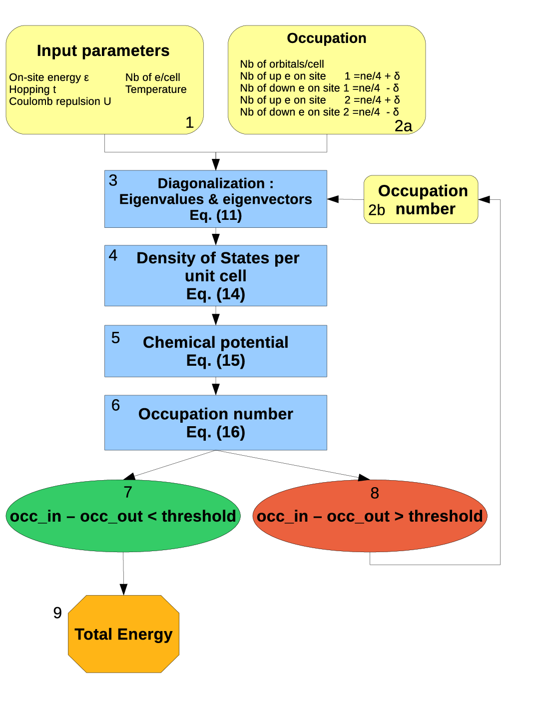
In order to find the ground-state energy for a given magnetic configuration, we need to employ a self-consistent scheme as, for a given spin $\sigma$, the energy depends on the mean occupation number of opposite spin, $\langle{\hat{n}}_{\alpha\bar{\sigma}}\rangle$, which in turns depends on the eigenvectors of the energy matrix itself. As shown in figure 3, we therefore start from a given configuration of input parameters (frames 1 and 2), we follow steps 3, 4, 5 and 6, up to the self-consistency condition expressed in frames 7 and 8, and finally move back to frame 2 or end to frame 9, depending on whether the condition is not satisfied or satisfied, respectively. The condition is satisfied when the output occupation number is the same as the input occupation number within a threshold that we fixed to $10^{-5}$.

In more details, we proceeded as follows: for practical reasons we found it simpler to numerically diagonalize the Hamiltonian of (III.2) through the Lapack libraries [6] (frame 3), in order to determine eigenvalues $\varepsilon_{j\sigma}(\vec{k})$ and eigenvectors $\Ket{\Psi^{\,j}_{\vec{k}\sigma}}=\sum_{\alpha}A^{\,j}_{\alpha,\sigma}(\vec{k})\Ket{\alpha\vec{k}}$ (with $j=1,2$). We actually work with the chemical potential in order to fix the particle density aposteriori: ${\hat{H}}_{H}^{\mu}={\hat{H}}_{H}-\mu\sum_{i\alpha\sigma}{\hat{n}}_{i\alpha\sigma}$. The calculations performed in frames 4, 5 and 6 are based on equations (16), (17) and (18) given below. The first of these equations expresses the DOS per unit cell, $\rho(\varepsilon)$:

The Dirac delta function in (16) is numerically calculated through a Gaussian function whose broadening is optimized after a convergence study: if the width of the Gaussian is too wide compared to the step between two energy points in $\varepsilon$, the DOS is too smooth, whereas if the width is too narrow, artificial oscillations appear. A more elegant approach might be to use the Methfessel-Paxton method [7], usually implemented in more advanced packages for electronic structure calculations.

As a second step we determine the chemical potential $\mu$ by the implicit equation:

Here $\beta=1/k_{B}T$ is the Boltzmann factor and we have defined the total number of electrons per unit cell (as used in figures 3, 5, 6): $n_{e}\equiv\sum_{\alpha,\sigma}\langle n_{\alpha\sigma}\rangle$. Finally, the average number of particles per site $\alpha$ and per spin $\sigma$ at a given temperature $T$ is given by:

At finite temperature, the thermodynamic variable to minimize is of course not the total energy, $E$, but the free energy, $F=E-TS$, what implies a calculation of the entropy of the system, through the equation:

Here $f(\varepsilon)$ is the Fermi-Dirac distribution. However, in what follows, we are interested in the ground-state phase diagram of the model, i.e., at $T=0$. We minimized therefore the total energy and used the parameter $T$ of equations (17) and (18) for convergence purposes only. It is in fact common practice to use a Fermi-Dirac distribution, characterized by a parameter $T$ different from zero, even in the $T\rightarrow 0$ limit, in order to smooth the step function that appears in equations (17) and (18) for $T=0$.

In general, we computed the total energy for each magnetic phase as a function of $t/U$. A phase transition is then characterized by the crossing of two (or more) free-energy curves: for example, we have represented the magnetic free energy as a function of $t/U$ in figure 4 for a specific occupation number ($n=0.8$), in order to highlight a magnetic (AFM/FM) transition. In this case the phase transition from AFM to FM phase is obtained at $t/U=0.13$, value at which the total FM energy becomes smaller than the AFM energy.

In figure 5, we have drawn the band structures for both FM and AFM phases to highlight the differences with the PM case. FM bands are shifted rigidly with respect to PM bands by about $\pm U\delta n$, where $\delta n$ is half the spin unbalance (see below). AFM bands are instead characterized by the opening of a gap that can be related to the difference $U(|\langle n_{1\bar{\sigma}}\rangle\!-\!\langle n_{2\bar{\sigma}}\rangle|)$ in (15). This gap leads to an insulating phase for $n_{e}=2.0$. It is important to notice that such a gap is not related to a metal-insulator transition (MIT) of the Mott-Hubbard kind, as it is not related to the electronic correlations (that are absent by definition in a mean-field calculation), but to magnetism. This MIT is rather called Slater MIT, in honor of J.C. Slater that foresaw it in 1951 [8]. In fact, differently from Mott that did not originally ascribed his MIT to magnetic interactions, Slater thought that the origin of the metal-to- insulator transition was determined by the onset of AFM long-range order, exactly as in the scheme described in the present paper. Therefore a Slater insulator is characterized by a band gap determined by a superlattice modulation of the magnetic periodicity. This is not the case of a Mott insulator.

Our main result is the ground-state phase diagram, drawn in Figure 6 as a function of the number of electrons per site and of $t/U$. Such a phase diagram had been already obtained in the literature in 1985 by Hirsch [9], though in a different context and without providing all the details of the derivation that can be found here. As a general feature the phase diagram shows a clear symmetry around half filling, i.e., one electron per site, where antiferromagnetism is the lowest-energy configuration. This symmetry had to be expected, since it is a symmetry of the Hubbard hamiltonian for nearest-neighbour hopping. Far from half-filling, paramagnetism is advantaged by a high value of $t/U$, whereas a low value of $t/U$ leads instead to ferromagnetism. This tendency for the PM/FM phases can be easily understood: the ground-state of $n$ non-interacting electrons ($U=0$) is PM because the minimum-energy constraint in combination with the Pauli principle forces to fill all the energy levels from the lowest ($\varepsilon_{\rm{min}}$) to the highest ($\mu$) with an equal number of $n/2$ up and $n/2$ down electrons. In the opposite extreme case, for $U/t\rightarrow\infty$, the system can gain energy by a total magnetization (say, all electrons with spin up), in order to minimize the energy term $U\langle n_{\downarrow}\rangle$. In the intermediate $t/U$ cases, only the numerical study of equations (III.2), (16), (17) and (18) can provide us with the magnetic phase of the system.

There exists however a criterion that allows us to foresee the stability of the PM phase versus the FM phase just on the base of the two parameters $U$ and $\rho(\mu)$, the DOS at the Fermi energy ($\varepsilon_{F}=\mu$ at $T=0$). This is Stoner criterion [10]. Start from the PM phase, represented in grey in figure 7(a) ($n_{\uparrow}=n_{\downarrow}=n/2$) and move $\delta n$ electrons from spin-down to spin-up states, so that $n_{\uparrow}=n/2+\delta n$ and $n_{\downarrow}=n/2-\delta n$. This leads to a shift of the chemical potential by $\pm\delta\varepsilon\simeq\pm\delta n/\rho(\mu)$ (if $\delta n\ll n$). The system is not at equilibrium, as $\mu_{\uparrow}=\mu+\delta n/\rho(\mu)\neq\mu_{\downarrow}=\mu-\delta n/\rho(\mu)$. Yet, because of the change in $\delta n$ and of the mean-field Coulomb energy (11), the minority-spin band shifts as a whole upward by $U\delta n+U(\delta n)^{2}/n$ and majority-spin band shifts as a whole downwards by $U\delta n-U(\delta n)^{2}/n$ as shown in figure 7(b).

In this situation, if ${\tilde{\mu}_{\uparrow}}=\mu+\delta n/\rho(\mu)-U\delta n+U(\delta n)^{2}/n$ is less than ${\tilde{\mu}_{\downarrow}}=\mu-\delta n/\rho(\mu)+U\delta n+U(\delta n)^{2}/n$, then it is favorable to still increase the number of spin-up electrons until ${\tilde{\mu}_{\uparrow}}={\tilde{\mu}_{\downarrow}}$. Therefore, ferromagnetism appears when ${\tilde{\mu}_{\uparrow}}\leq{\tilde{\mu}_{\downarrow}}$. This leads to the Stoner criterion for ferromagnetic stability:

Equation 20 can also be written as $\frac{t}{U}\leq t\rho(\mu)$. The corresponding equality, that marks the phase transition, has been reproduced in figure 6. All our calculated points for the PM/FM transition lie on the theoretical curve $\frac{t}{U}=t\rho(\mu)$ represented by a dotted line in Figure 6. We infer from the Stoner criterion that a ferromagnetic instability is expected in materials showing a high density of states at Fermi level. This is indeed the case for Fe, Co and Ni [11]. It is also possible to find a similar criterion for the AFM/PM and AFM/FM transitions, but its derivation is technically more involved because it is based on a Bogoliubov transformation. This leads to a gap-equation formally equivalent to the one of the BCS theory of superconductivity. A rather detailed description of this generalization can be found in [12].

References

- [1] J. Hubbard. Electron correlations in narrow energy bands. Proc. Roy. Soc. London, Ser. A, 276(1365):238–257, 1963.
- [2] J. Hubbard. Electron correlations in narrow energy bands. ii. the degenerate band case. Proc. Roy. Soc. London, Ser. A, 277(1369):237–259, 1964.
- [3] J. Hubbard. Electron correlations in narrow energy bands. iii. an improved solution. Proc. Roy. Soc. London, Ser. A, 281(1386):401–419, 1964.
- [4] A basic introduction to the second-quantisation formalism can be found in: Ph. A. Martin, F. Rothen, Many-Body problems and quantum field theory: an introduction, (Springer, 2004), or a more advanced one in A. L. Fetter and J. D. Walecka, Quantum theory of many-particle systems, (McGraw-Hill, 1971).
- [5] N.W. Ashcroft and N.D. Mermin. Solid state physics. Holt, Rinehart and Winston; Saunders, 1976.
- [6] Linear Algebra PACKage can be found at the address: http://www.netlib.org/lapack.
- [7] M. Methfessel and A. T. Paxton. High-precision sampling for brillouin-zone integration in metals. Phys. Rev. B, 40:3616–3621, Aug 1989.
- [8] J. C. Slater. Magnetic effects and the hartree-fock equation. Phys. Rev., 82:538–541, May 1951.
- [9] J. E. Hirsch. Two-dimensional hubbard model: Numerical simulation study. Phys. Rev. B, 31:4403–4419, Apr 1985.
- [10] E. C. Stoner. Collective electron specific heat and spin paramagnetism in metals. Proc. Roy. Soc. London, Ser. A, 154(883):656–678, 1936.
- [11] S. Blundell. Magnetism in condensed matter. Oxford University Press, Oxford, 2001.
- [12] G.D. Mahan. Many Particle Physics. Springer, 3d edition, 2000.
- [13] D. H. Lee, R. G. Caflisch, J. D. Joannopoulos, and F. Y. Wu. Antiferromagnetic classical model: A mean-field analysis. Phys. Rev. B, 29:2680–2684, Mar 1984.
- [14] H. Q. Lin and J. E. Hirsch. Two-dimensional hubbard model with nearest- and next-nearest-neighbor hopping. Phys. Rev. B, 35:3359–3368, Mar 1987.
- [15] S. Di Matteo, N. B. Perkins, and C. R. Natoli. Spin-1 effective hamiltonian with three degenerate orbitals: An application to the case of V2O3. Phys. Rev. B, 65:054413, Jan 2002.
- [16] P. W. Anderson. Localized magnetic states in metals. Phys. Rev., 124:41–53, Oct 1961.
- [17] V. J. Emery. Theory of high-Tc superconductivity in oxides. Phys. Rev. Lett., 58:2794–2797, Jun 1987.
- [18] C. M. Varma. Non-fermi-liquid states and pairing instability of a general model of copper oxide metals. Phys. Rev. B, 55:14554–14580, Jun 1997.
- [19] Louis Felix Feiner and Andrzej M. Oleś. Electronic origin of magnetic and orbital ordering in insulating . Phys. Rev. B, 59:3295–3298, Feb 1999.
- [20] Masatoshi Imada, Atsushi Fujimori, and Yoshinori Tokura. Metal-insulator transitions. Rev. Mod. Phys., 70:1039–1263, Oct 1998.
- [21] V.V. Val’kov S.G. Ovchinnikov. Hubbard operators in the theory of strongly correlated electrons. Imperial College Press, 2004.
- [22] Vladimir I. Anisimov, Jan Zaanen, and Ole K. Andersen. Band theory and mott insulators: Hubbard u instead of stoner i. Phys. Rev. B, 44:943–954, Jul 1991.
- [23] Vladimir I Anisimov, F Aryasetiawan, and A I Lichtenstein. First-principles calculations of the electronic structure and spectra of strongly correlated systems: the lda + u method. Journal of Physics: Condensed Matter, 9(4):767, 1997.
- [24] Gironcoli S. Himmetoglu B., Floris A. and Cococcioni M. Hubbard-corrected dft energy functionals: The lda+u description of correlated systems. Int. J. Quantum Chem., 114:14–49, Aug 2014.
- [25] Antoine Georges, Gabriel Kotliar, Werner Krauth, and Marcelo J. Rozenberg. Dynamical mean-field theory of strongly correlated fermion systems and the limit of infinite dimensions. Rev. Mod. Phys., 68:13–125, Jan 1996.
- [26] G. Kotliar, S. Y. Savrasov, K. Haule, V. S. Oudovenko, O. Parcollet, and C. A. Marianetti. Electronic structure calculations with dynamical mean-field theory. Rev. Mod. Phys., 78:865–951, Aug 2006.