The Trihydrogen cation $H_{3}^{+}$ was identified, by mass spectroscopy, in 1911 by J.J. Thomson[1]. Twelve years later Hogness and Lunn[2] found that it could be produced by the proton exchange $H_{2}^{+}+H_{2}\rightarrow H_{3}^{+}+H$ and would readily lose an electron. Subsequently it was found that $H_{3}^{+}$ is present in interstellar clouds and is among the most abundant molecular species in the universe. This led to the question of the stability of the dication $H_{2}^{++}$, which has remained somewhat controversial to the present, though the consensus is that it is unstable.

The first quantum treatment was by Gordadse[3, 4] in (1935), who assumed the protons were fixed, equally spaced along a straight line or formed an equilateral triangle. He used the variational method, as have all subsequent studies, based on a one-parameter trial function built from the hydrogen 1s-state. In spite of the simplicity of the trial functions, he found several of the multi-center integrations intractable, requiring not too well controlled approximations, and concluded that neither configuration was stable. About the same time C.A. Coulson carried out a LCMO study of $H_{3}^{++}$ [5]. He used only a single molecular orbital and his energy values lie somewhat higher than those in [4]. The difficulty of these multi-center integrations have continued to dog such calculations and may be what prompted Eyring’s comment that $H_{3}^{+}$ is “the scandal of modern chemistry” [6]. The first extensive study of $H_{3}^{++}$ using electronic digital computers was by H. Conroy in 1964 [7,8,9,10], who devised an insightful set of variational wave functions and used Monte-Carlo algorithms for the integrations, remarking that “these integrations presented grave obstacles”. This and subsequent calculations [11,12,13,14,15], mostly confined to the linear and equilateral triangle configurations, have upheld Gordadse’s conclusion that the ion is unstable. An attempt to produce the dication experimentally [16, 17] was unsuccessful.

The purpose of this note is to suggest that it is possible to avoid the variational method and consequent multi-center integrations entirely and that the Schroedinger equation can be solved exactly for a sequence of Hamiltonians that converge to the correct one. This note is intended as a proof of principle, and deals only with the first Hamiltonian in the sequence; it is equivalent to keeping only the hydrogen 1s state and is simple enough that most of the calculations can be done “by hand”. We also assume that the ion forms an isosceles triangle and the ground-state energy (ignoring hyperfine effects) is examined as a function of a side and adjacent angle. Even so, the results lie reasonably close to the most recent values.

Let the one-electron Hamiltonian of an atom ( or indeed, any system) be

$$H=p^{2}+V(\vec{r})$$

$(1.1)$

and have bound-state eigenfunctions and energy levels $\{\phi_{a},\;E_{a}\}$. Then, by completeness,

$$V(\vec{r})=\sum_{a}v_{a}(\vec{r})<\phi_{a}|,\qquad v_{a}(\vec{r})=V(\vec{r})|\phi_{a}>.$$

$(1.2)$

Thus, if we ignore the continuum states, which will be of no interest in the sequel, then we have a sequence of Hamiltonians

$$H_{n}=p^{2}+\sum_{m=0}^{n}v_{m}<\phi_{m}|$$

$(1.3)$

and it is easily checked that the Schroedinger equation (we adopt units: $\hbar=2m=e^{2}/2=1$)

$$\{-\nabla^{2}-E\}\psi(\vec{r})=-\sum_{m=0}^{n}v_{m}(\vec{r})\lambda_{m}$$

$$\lambda_{m}=\int d\vec{s}\phi_{m}^{*}(\vec{s})\psi(\vec{s})$$

$(1.4)$

has precisely the first $n$ of the eigenstates of $H$. By transforming to momentum space and writing $E=-\epsilon<0$ (since we are only concerned with bound states) (4) becomes the integral equation

$$\hat{\psi}(\vec{k})=\sum_{m=0}^{n}\frac{\hat{v}_{m}(\vec{k})\lambda_{m}}{\epsilon+k^{2}}.$$

$(1.5)$

Next, by the Parseval relation for the Fourier transform [2] we have the consistency condition

$$\lambda_{q}=\frac{1}{(2\pi)^{3}}\int\hat{\phi}_{q}^{*}(\vec{k})\hat{\psi}(\vec{k})d\vec{k}=\sum_{m}A_{qm}\lambda_{m}$$

$$A_{qm}=\frac{1}{(2\pi)^{3}}\int\frac{\hat{v}_{m}(\vec{k})\hat{\phi}_{q}^{*}(\vec{k})}{k^{2}+\epsilon}d\vec{k}.$$

$(1.6)$

That is to say, the energy levels $\epsilon$ and corresponding $\lambda$’s are determined by the matrix equations

$$({\bf A}-{\bf I})\Lambda=0,\qquad Det|{\bf A}-{\bf I}|=0$$

$(1.7)$

where $\Lambda$ is the column vector $(\lambda_{0},\cdots,\lambda_{n})^{T}$. In the next section we illustrate this by working out $H_{0}$ and $H_{1}$ for hydrogen.

It should be pointed out that in (1.2) the $\phi_{a}$ may be any complete set of functions, not just the eigenfunctions of $H$, though the low order approximations are unlikely to be as accurate.

Consider the three-proton system, in the Born-Oppenheimer approximation, where one lies at the origin and two lie in the $x-z$-plane at positions

$$\vec{R}_{\pm}=R(\cos\alpha,0,\pm\sin\alpha).$$

$(3.1)$

The Schroedinger equation for an electron subject to this configuration is

$$-(\nabla^{2}+E)\psi(\vec{r})=[V(\vec{r})+V(\vec{r}-\vec{R}_{+})+V(\vec{r}-\vec{R}_{-})]\psi(\vec{r}).$$

$(3.2)$

Setting $E=-\epsilon$, (3.2) has the immediate solution in momentum space

$$\hat{\psi}(\vec{k})=\frac{\hat{v}_{0}(\vec{k})}{k^{2}+\epsilon}[\lambda_{0}+e^{i\vec{k}\cdot\vec{R}_{+}}\lambda_{+}+e^{i\vec{k}\cdot\vec{R}_{-}}\lambda_{-}]$$

$(3.3)$

with

$$\lambda_{0}=\frac{1}{(2\pi)^{3}}\int d\vec{k}\hat{\phi}_{0}(\vec{k})^{*}\hat{\psi}(\vec{k})$$

$$\lambda_{\pm}=\frac{1}{(2\pi)^{3}}\int d\vec{k}\hat{\phi}_{0}(\vec{k})^{*}e^{-i\vec{k}\cdot\vec{R}_{\pm}}\hat{\psi}(\vec{k}).$$

$(3.4)$

Therefore, by defining the four integrals

$$I_{0}=\frac{1}{(2\pi)^{3}}\int d\vec{k}\frac{\hat{\phi}_{0}^{*}(\vec{k})\hat{v}_{0}(\vec{k})}{k^{2}+\epsilon}$$

$$I_{\pm}=\frac{1}{(2\pi)^{3}}\int d\vec{k}\frac{\hat{\phi}_{0}^{*}(\vec{k})\hat{v}_{0}(\vec{k})}{k^{2}+\epsilon}e^{i\vec{k}\cdot\vec{R}_{\pm}}$$

$(3.5)$

$$I_{1}=\frac{1}{(2\pi)^{3}}\int d\vec{k}\frac{\hat{\phi}_{0}^{*}(\vec{k})\hat{v}_{0}(\vec{k})}{k^{2}+\epsilon}e^{-i\vec{k}\cdot(\vec{R}_{+}-\vec{R}_{-})},$$

we have the three consistency equations

$$\lambda_{0}=I_{0}\lambda_{0}+I_{+}\lambda_{+}+I_{-}\lambda_{-}$$

$$\lambda_{+}=I_{+}^{*}\lambda_{0}+I_{0}\lambda_{+}+I_{1}\lambda_{-}$$

$(3.6)$

$$\lambda_{-}=I_{-}\lambda_{0}+I_{1}^{*}\lambda_{+}+I_{0}\lambda_{-}.$$

The four integrals (3.5) are real, $I_{+}=I_{-}$ and is independent of $\alpha$. From (3.6) we see that the ground state energy $\epsilon$ is fixed by the determinantal equation ($\epsilon=x^{2})$

$$F[R,\epsilon]\equiv(I_{0}-I_{1}-1)[(I_{0}-1)^{2}+(I_{0}-1)I_{1}-2I_{+}^{2}]=0.$$

$(3.7)$

The integrals (3.5) are elementary:

$$I_{0}=\frac{2(3+x)}{(1+x)^{3}}$$

$$I_{\pm}=f(R,x)=\frac{16}{(x^{2}-1)^{2}}\left\{\frac{e^{-R}-e^{-Rx}}{R(x^{2}-1)}+\frac{1}{8}e^{-R}[x^{2}-5+R(x^{2}-1)]\right\}$$

$(3.8)$

$$I_{1}=f(2R\sin\alpha,x).$$

The spatial wave function is obtained through the Fourier inversion of (3.3) by which we find in spherical coordinates

$$\psi(r,\theta,\phi)=$$

$$N\left\{\frac{e^{-r}-e^{-xr}}{r}+\left(\frac{1-I_{0}}{2I_{+}}\right)\left[\frac{e^{-\rho_{+}}-e^{-x\rho_{+}}}{\rho_{+}}+\frac{e^{-\rho_{-}}-e^{-x\rho_{-}}}{\rho_{-}}\right]\right\},$$

$(3.9)$

where $N$ is a normalization factor and

$$\rho_{\pm}=\sqrt{r^{2}+r^{2}-2rR(\sin\theta\cos\varphi\cos\alpha\pm\cos\theta\sin\alpha)}.$$

$(3.10)$

The wave function in the equilateral triangle configuration for $r=R=1.6$, is shown as a function of $\theta$ and $\varphi$ in Fig.1.

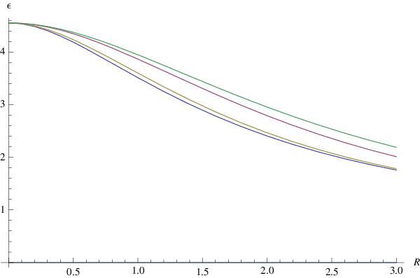
The ground state energy $E=-\epsilon=-x^{2}$ is given by the largest positive root $x$ of (3.7) which is that of the second factor. This is most easily determined graphically and the results for four cases are given below.

References

- [1] J.J. Thomson, Proc. Roy. Soc(Lond)A89, 1 (1913).
- [2] T.R. Hogness and E.G. Lunn, Phys. Rev.26, 44 (1925).
- [3] G.S. Gordadse, Z.f. Physik 96, 542 (1935).
- [4] G.S. Gordadse, Z.f. Physik 99,284 (1936).
- [5] C.A. Coulson, Proc. Camb. Phil. Soc. 31, 244 (1935).
- [6] G.S. Handler and J.R. Arnold, J. Chem. Phys.27, 144 (1957).
- [7] H. Conroy, J. Chem. Phys.41, 1327 (1964).
- [8] H. Conroy, J. Chem. Phys.41, 1331 (1964).
- [9] H. Conroy, j. Chem. Phys.41, 1336 (1964).
- [10] H. Conroy, J. Chem. Phys.51, 3979 (1964).
- [11] K. Matsubara, Bul. Nara U. Edu.18, 7 (1969).
- [12] R.L. Samorjai and C.P. Yue, J. Chem. Phys.53, 1657 (1970).
- [13] R.M. Shoucri and B.T. Darling, J. Chem. Phys.56, 1789 (1973).
- [14] J. Hernandez and R. Carbo, J. Chem. Phys.62, 2637 (1975).
- [15] J. Ackermann, B. Erdmann and R. Raltzsch, J. Chem. Phys. 101,7 648 (1994).
- [16] N. Papp and L. Kervin, Phys.Rev. Lett.23, 1743 (1969).
- [17] E.H. Berkowitz and H. Stocker, J. Chem. Phys.55, 4606 (1971).
- [18] H. Medel-Cobaxin, A. Alijah and A.V. Turbiner, Coll.Czech Chem. Commun.73,1271 (2008).
- [19] A.R. Levin, Reformulation of the Muffin-Tin Problem in Electronic Structure Calculations within the FEAST Framework, [ Ph.D. Thesis, University of Massachusetts, Amherst (2012)].
- [20] M.L. Glasser, Relativistic ground-state of the hydrogen molecular ion, Unpublished report.
- [21] A.V. Turbiner and J.C. Lopez Vieyra, Phys. Rpts.424, 309 (2006).