Diversity of Linear Transceivers in MIMO AF Half-duplex Relaying Channels Thanks: This work was supported in part by FP7 project PHYLAWS (EU FP7-ICT 317562) and partially submitted to IEEE International Symposium on Information Theory (ISIT) 2014. The authors are with the Department of Electrical and Electronic Engineering, Imperial College, London, UK (e-mail: {csong and c.ling}@imperial.ac.uk).

Changick Song and Cong Ling Affiliation:

Abstract

Linear transceiving schemes between the relay and the destination have recently attracted much interest in MIMO amplify-and-forward (AF) relaying systems due to low implementation complexity. In this paper, we provide comprehensive analysis on the diversity order of the linear zero-forcing (ZF) and minimum mean squared error (MMSE) transceivers. Firstly, we obtain a compact closed-form expression for the diversity-multiplexing tradeoff (DMT) through tight upper and lower bounds. While our DMT analysis accurately predicts the performance of the ZF transceivers, it is observed that the MMSE transceivers exhibit a complicated rate dependent behavior, and thus are very unpredictable via DMT for finite rate cases. Secondly, we highlight this interesting behavior of the MMSE transceivers and characterize the diversity order at all finite rates. This leads to a closed-form expression for the diversity-rate tradeoff (DRT) which reveals the relationship between the diversity, the rate, and the number of antennas at each node. Our DRT analysis compliments our previous work on DMT, thereby providing a complete understanding on the diversity order of linear transceiving schemes in MIMO AF relaying channels.

I Introduction

Recently, there has been growing interest in multiple-input multiple-output (MIMO) relaying techniques, due to combined benefits of improved link performance from MIMO channels and coverage extension from relaying techniques. In particular, although suboptimal, linear transceivers between the relay and the destination with the amplify-and-forward (AF) strategy have attracted much attention for its low complexity implementation [1, 2, 3, 4, 5]. From a system design perspective, in order to find the operating points of the system and predict its performance, analytical research on these transceiving schemes is highly motivated [6, 7, 8, 9, 10], but the performance has not been fully understood yet.

The “diversity-multiplexing tradeoff” (DMT) analysis provides a fundamental criterion to evaluate the performance of MIMO systems since it compactly characterizes the tradeoff between the rate and the block error probability [11]. For this reason, a large amount of research has been conducted in MIMO relaying systems based on the DMT [12, 13, 14, 15, 16, 17, 18, 19]. With the minimum mean squared error (MMSE) strategy, however, the DMT is not sufficient to characterize the diversity order, because the DMT framework, as an asymptotic notion in the high signal-to-noise ratio (SNR) and high spectral efficiency regime, cannot distinguish between different spectral efficiencies that correspond to the same multiplexing gain which we denote by $r$ . In fact, it was shown in point-to-point (P2P) MIMO channels that while the DMT analysis accurately predicts the diversity behavior of the MMSE receiver for the positive multiplexing gain ( $r>0$ ), the extrapolation of the DMT to $r=0$ is unable to predict the performance especially at low rates. This rate-dependent behavior of MMSE receivers has first been observed by Hedayat et al. in [20] and comprehensively analyzed by Mehana et al. in [21]. A similar phenomenon can be observed in MIMO AF relaying systems, but the analysis has not been made so far.

In the first part of the paper, we introduce a new design framework for linear transceiver optimization in MIMO AF relaying systems utilizing the error covariance decomposition (ECD). We would like to mention that the ECD approach was first suggested in [2] for designing the MMSE transceiver under the assumption that the number of data-streams is smaller than or equal to that of relay and destination antennas. In fact, however, any restriction on the antenna configuration is unnecessary under the MMSE strategy, because a certain diversity gain is always achievable as the rate becomes smaller (this phenomenon will be addressed later in the analysis part). Therefore, it is important to provide a new result of the ECD that can be applied to any kinds of antenna configurations. We remark that our new approach not only generalizes the previous work in [2], but also provides a ECD framework which brings the ZF and MMSE strategies together.

In the second part of the paper, we present asymptotic analysis of the aforementioned linear transceivers. We first focus on the DMT performance of the systems. Previously, some DMT bounds have been found in [10] for the MMSE transceiver, but they are loose in general. In this paper, we characterize the exact DMT performance of the ZF and MMSE transceivers as a closed-form expression through deriving tight upper and lower bounds. Note that for the sake of comparison, our analysis also covers the naive schemes where only a constant gain factor is applied at the relay without channel state information (CSI). The resulting DMT reveals that all linear transceiving and naive schemes are suboptimal in terms of the achievable diversity in MIMO relaying channels [16] [17]. It is also shown that while the DMT is determined by the first-hop link for the linear transceivers, the naive schemes depend on the minimum DMT of the first-hop and second-hop MIMO links, which implies that the naive scheme is always inferior to the transceiving scheme, especially when the number of relay antennas is large.

While our DMT analysis accurately predicts the ZF transceivers, it is observed that when the rate is finite, the MMSE transceivers exhibit a complicated rate dependent behavior, and thus are very unpredictable via DMT. To address this issue, we alternatively approach the outage probability of the MMSE transceiver by setting the multiplexing gain zero. This leads to a closed-form expression for the diversity-rate tradeoff (DRT) which reveals the relationship between the diversity, spectral efficiency, and the number of antennas at each node. We note that under the DRT formulation, the analysis must be conducted more carefully compared to the DMT since certain ratios and terms that were simply ignored in the DMT analysis may be relevant. The presented bounds are tight except some discontinuity rate points, and thus can precisely predict the diversity behavior of the MMSE transceiver. Interestingly, we observe that as the rate becomes smaller, the MMSE transceiver approaches the maximum likelihood (ML) performance [22] [23] with full-diversity order of the MIMO relay channel. In contrast, however, the full-diversity order may not be achievable with the naive-MMSE scheme no matter how small the rate is, which reveals the importance of the CSI at the relay for obtaining a proper diversity gain in MMSE-based relaying systems. Our DMT and DRT analyses are complementary to each other, thereby allowing us to obtain a complete understanding on the diversity order of the linear transceivers in MIMO AF relay channels. Finally, some simulations results are presented to demonstrate the accuracy of the analysis.

Notations: Throughout this paper, normal letters represent scalar quantities, boldface letters indicate vectors and boldface uppercase letters designate matrices. $\mbox{$\bf I$}_{N}$ is an $N\times N$ identity matrix We use $\mathbb{C}$ and $\mathbb{S}_{+}^{M}$ to denote a set of complex numbers and $M\times M$ positive definite matrices, respectively. $\preceq$ or $\succeq$ represent generalized inequality defined on the positive definite cone. In addition, $E[\cdot]$ , $(\cdot)^{H}$ , $(\cdot)^{+}$ , $\lceil\cdot\rceil$ , and $\lfloor\cdot\rfloor$ stand for expectation, conjugate transpose, $\max(\cdot,0)$ , rounding up, and down operations, respectively. $[\mbox{$\bf A$}]_{k,k}$ and $\textrm{Tr}\left(\mbox{$\bf A$}\right)$ denote the $k$ -th diagonal element and trace function of a matrix $\bf A$ . The $k$ -th element of a vector $\bf a$ is denoted by $a_{k}$ . We denote $f(\rho)\doteq g(\rho)$ , when two functions $f(\rho)$ and $g(\rho)$ are exponentially equal as $\lim_{\rho\rightarrow\infty}\frac{\log f(\rho)}{\log\rho}=\lim_{\rho\rightarrow\infty}\frac{\log g(\rho)}{\log\rho}$ . Inequalities $\dot{\leq}$ and $\dot{\geq}$ are similarly defined.

II System Model

Refer to caption — Fig. 1: Joint encoding/decoding structure for MIMO AF relaying channels with linear transceivers

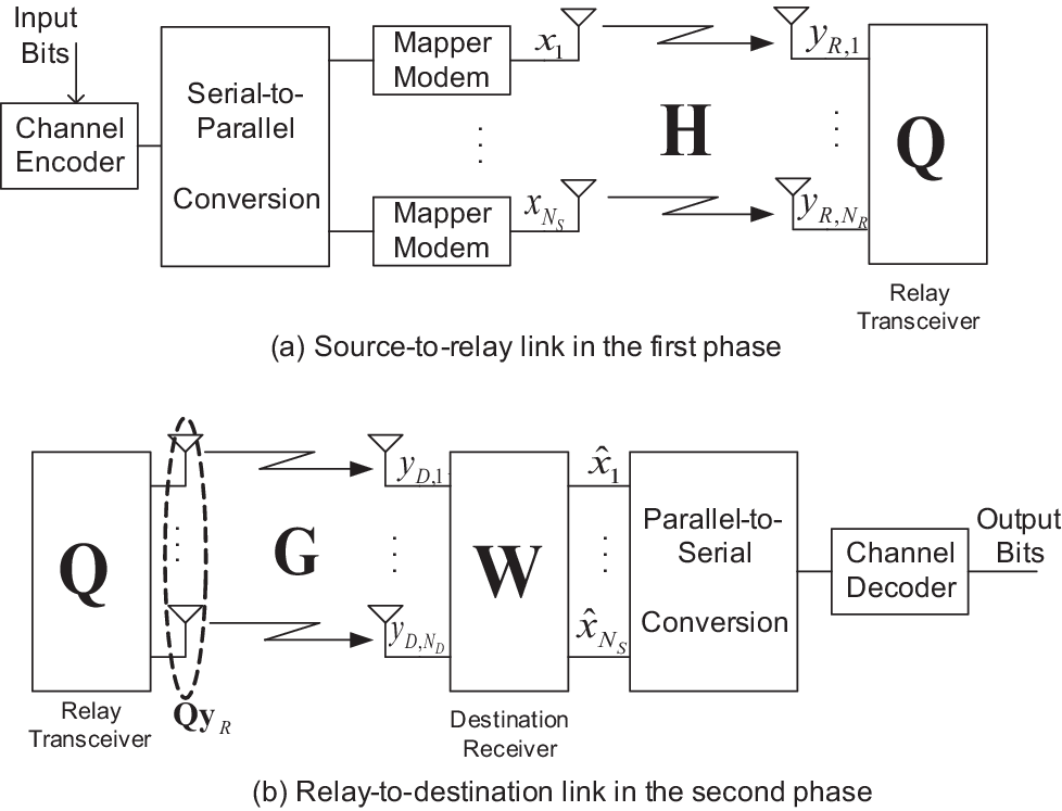
In this paper, we consider quasi-static flat fading MIMO AF relaying channels equipped with $N_{S}$ , $N_{R}$ , and $N_{D}$ number of antennas at the source, the relay, and the destination, respectively. A direct link between the source and the destination is ignored due to large pathloss. We assume the half-duplex relay, which means that each data transmission occurs in two separate phases (time or frequency). We assume that no channel state information (CSI) is available at the source, but the global CSI, i.e., perfect knowledge of both $\bf H$ and $\bf G$ is allowed at the destination. The relay can be informed of either the global CSI or no CSI.

In the first phase, the output of the underlying MIMO channel between the source and the relay can be expressed as $\mbox{$\bf y$}_{R}=\mbox{$\bf H$}\mbox{$\bf x$}+\mbox{$\bf n$}_{R}$ , where $\mbox{$\bf x$}\in\mathbb{C}^{N_{S}\times 1}$ , $\mbox{$\bf H$}\in\mathbb{C}^{N_{R}\times N_{S}}$ and $\mbox{$\bf n$}_{R}\in\mathbb{C}^{N_{R}\times 1}$ represent the input signal vector, the channel matrix between the source and the relay, and the noise vector at the relay, respectively. Denoting the total transmit power at the source by $P_{S}$ , we suppose that each source antenna uses equal power $\rho\triangleq E[|x_{k}|^{2}]=P_{S}/N_{S}$ for all $k$ because of no CSI at the source.

In the second phase, the relay signal $\mbox{$\bf y$}_{R}$ is amplified by the relay matrix $\mbox{$\bf Q$}\in\mathbb{C}^{N_{R}\times N_{R}}$ and transmitted to the destination. Then, the standard baseband signal at the destination is written by

\displaystyle\mbox{$\bf y$}_{D}=\mbox{$\bf G$}\mbox{$\bf Q$}\mbox{$\bf y$}_{R}+\mbox{$\bf n$}_{D}=\mbox{$\bf G$}\mbox{$\bf Q$}\mbox{$\bf H$}\mbox{$\bf x$}+\mbox{$\bf G$}\mbox{$\bf Q$}\mbox{$\bf n$}_{R}+\mbox{$\bf n$}_{D},

(1)

where $\mbox{$\bf n$}_{D}$ designates the noise vector at the destination. Note that the relay matrix $\bf Q$ must satisfy the relay power constraint $P_{R}$ as $E[\|\mbox{$\bf Q$}\mbox{$\bf y$}_{R}\|^{2}]\leq P_{R}$ . Finally, when a linear equalizer $\mbox{$\bf W$}\in\mathbb{C}^{N_{S}\times N_{D}}$ is employed at the destination, the estimated signal waveform $\hat{\mbox{$\bf x$}}\in\mathbb{C}^{N_{S}\times 1}$ is expressed as $\hat{\mbox{$\bf x$}}=\mbox{$\bf W$}\mbox{$\bf y$}_{D}$ .

As the equalizer $\bf W$ decouples the received signal into $N_{S}$ parallel data streams, the transmit signals at the source can be encoded either jointly or separately. To be specific, the joint encoding indicates the case in which a single channel encoder supports all the data streams at the source so that coding is applied jointly across antennas as illustrated in Figure 1. Hence, this coding scheme is advantageous to attain the diversity gain of MIMO channels. In contrast, the separate encoding drives $N_{S}$ data streams independently using $N_{S}$ encoders, the outputs of which are fed to $N_{S}$ independent decoders; thus, is based sorely on the spatial multiplexing.

In this work, we make a standard assumption that all entries of channel matrices $\bf H$ and $\bf G$ are independent and identically distributed (i.i.d.) $\sim\mathcal{CN}(0,1)$ and remain constant during the transmission of a codeword. All elements of the noise vectors $\mbox{$\bf n$}_{R}$ and $\mbox{$\bf n$}_{D}$ are also assumed to be i.i.d. $\sim\mathcal{CN}(0,1)$ . Finally, we define the following eigenvalue decompositions $\mbox{$\bf H$}^{H}\mbox{$\bf H$}=\mbox{$\bf U$}_{h}\mathbf{\Lambda}_{h}\mbox{$\bf U$}_{h}^{H}$ and $\mbox{$\bf G$}^{H}\mbox{$\bf G$}=\mbox{$\bf U$}_{g}\mathbf{\Lambda}_{g}\mbox{$\bf U$}_{g}^{H}$ , where $\mbox{$\bf U$}_{h}\in\mathbb{C}^{N_{S}\times N_{S}}$ and $\mbox{$\bf U$}_{g}\in\mathbb{C}^{N_{R}\times N_{R}}$ are unitary matrices, and $\mathbf{\Lambda}_{h}\in\mathbb{C}^{N_{S}\times N_{S}}$ and $\mathbf{\Lambda}_{g}\in\mathbb{C}^{N_{R}\times N_{R}}$ represent square diagonal matrices with eigenvalues $\lambda_{h,i}$ for $i=1,\ldots,N_{S}$ and $\lambda_{g,j}$ for $j=1,\ldots,N_{R}$ , respectively. All eigenvalues are arranged in descending order.

III Linear Transceivers

We would like to mention that the optimal MMSE transceiver between the relay and the destination was first developed in [1]. However, it is known that the approach in [1] which is based on the singular-value decomposition (SVD) is cumbersome to deal with due to the complicated structure of a compound channel matrix and colored noise at the destination. In this section, we introduce an alternative design method utilizing the ECD property, which makes the analysis more tractable. Our approach extends the previous result in [2] and provides a ECD framework which brings the ZF and MMSE strategies together.

III-A MMSE Transceiver

We start by defining the error vector $\mbox{$\bf e$}\triangleq\hat{\mbox{$\bf x$}}-\mbox{$\bf x$}$ and its covariance matrix $\mbox{$\bf R$}_{e}\triangleq E[\mbox{$\bf e$}\mbox{$\bf e$}^{H}]$ . Then, the joint MMSE optimization problem for $\bf Q$ and $\bf W$ is written by

\displaystyle\min_{\mathbf{Q,W}}\text{Tr}\left(\mbox{$\bf R$}_{e}\right)~~s.t.~~\text{Tr}\left(\mbox{$\bf Q$}(\rho\mbox{$\bf H$}\mbox{$\bf H$}^{H}+\mbox{$\bf I$}_{N_{R}})\mbox{$\bf Q$}^{H}\right)\leq P_{R}.

(2)

The problem is unconstrained and convex with respect to $\bf W$ , and thus the solution for $\bf W$ is easily obtained as the Wiener filter, i.e.,

\displaystyle\hat{\mbox{$\bf W$}}_{\text{WF}}=\rho\mbox{$\bf H$}^{H}\mbox{$\bf Q$}^{H}\mbox{$\bf G$}^{H}(\rho\mbox{$\bf G$}\mbox{$\bf Q$}\mbox{$\bf H$}\mbox{$\bf H$}^{H}\mbox{$\bf Q$}^{H}\mbox{$\bf G$}^{H}+\mbox{$\bf R$}_{n})^{-1},

(3)

where $\mbox{$\bf R$}_{n}\triangleq\mbox{$\bf G$}\mbox{$\bf Q$}\mbox{$\bf Q$}^{H}\mbox{$\bf G$}^{H}+\mbox{$\bf I$}_{N_{D}}$ designates the covariance matrix of the effective noise $\mbox{$\bf n$}\triangleq\mbox{$\bf G$}\mbox{$\bf Q$}\mbox{$\bf n$}_{R}+\mbox{$\bf n$}_{D}$ . Therefore, a principal issue of the problem (2) is to find $\bf Q$ . The following lemma shows that with the MMSE strategy, the optimal relay matrix takes a particular structure.

Lemma 1

The optimal relay matrix $\bf Q$ of the problem (2) is generally expressed as a product of two matrices

\displaystyle\hat{\mbox{$\bf Q$}}=\mbox{$\bf B$}\mbox{$\bf L$},

(4)

where $\mbox{$\bf B$}\in\mathbb{C}^{N_{R}\times N_{S}}$ is an unknown matrix as of yet, but $\mbox{$\bf L$}\in\mathbb{C}^{N_{S}\times N_{R}}$ is a matrix which is given by $\mbox{$\bf L$}=\mbox{$\bf P$}\mbox{$\bf H$}^{H}$ with $\mbox{$\bf P$}\in\mathbb{C}^{N_{S}\times N_{S}}$ being an arbitrary square invertible matrix.

Proof:

See Appendix A. ∎

Let us set $\mbox{$\bf P$}=(\mbox{$\bf H$}^{H}\mbox{$\bf H$}+\rho^{-1}\mbox{$\bf I$}_{N_{S}})^{-1}$ so that $\bf L$ forms the MMSE receiver for the first-hop channel $\bf H$ with the input signal $\bf x$ . Now, we define $\mbox{$\bf y$}\triangleq\mbox{$\bf L$}\mbox{$\bf y$}_{R}\in\mathbb{C}^{N_{S}\times 1}$ as the output signal of the relay receiver $\bf L$ , and its covariance matrix $\mbox{$\bf R$}_{y}\triangleq E[\mbox{$\bf y$}\mbox{$\bf y$}^{H}]\in\mathbb{C}^{N_{S}\times N_{S}}$ as

\displaystyle\mbox{$\bf R$}_{y}=\mbox{$\bf L$}(\rho\mbox{$\bf H$}\mbox{$\bf H$}^{H}+\mbox{$\bf I$}_{N_{R}})\mbox{$\bf L$}^{H}.

(5)

Then, the estimated signal vector $\hat{\mbox{$\bf x$}}$ and the relay power constraint in (2) are respectively rephrased as

\displaystyle\hat{\mbox{$\bf x$}}=\mbox{$\bf W$}(\mbox{$\bf G$}\mbox{$\bf B$}\mbox{$\bf y$}+\mbox{$\bf n$}_{D})~~\text{and}~~\text{Tr}(\mbox{$\bf B$}\mbox{$\bf R$}_{y}\mbox{$\bf B$}^{H})\leq P_{R}.

(6)

Since the rank of $\mbox{$\bf R$}_{y}$ equals $M\triangleq\min(N_{S},N_{R})$ , $\mbox{$\bf R$}_{y}$ becomes clearly non-invertible when $N_{S}>N_{R}$ . This fact makes the problem more challenging, but has not been fully addressed in conventional literature. In the following, we revisit the previous works in [1] and [2], and provide a more generalized and insightful design strategy without restriction on the number of antennas at the source.

In fact, when the relay receiver $\bf L$ forms the MMSE receiver for the first hop channel, one can show that the error covariance matrix $\mbox{$\bf R$}_{e}$ in (2) is expressed as a sum of two individual covariance matrices, each of which represents the first hop and the second hop MIMO channels, respectively. This result has been proved in [2], but the proof was limited to the cases of $N_{S}\leq\min(N_{R},N_{D})$ . For the sake of completeness, we give a new result of error decomposition that can be applied to any kind of antenna configurations.

Lemma 2

Define the eigenvalue decomposition $\mbox{$\bf R$}_{y}=\mbox{$\bf U$}_{h}\mathbf{\Lambda}_{y}\mbox{$\bf U$}_{h}^{H}$ where $\mathbf{\Lambda}_{y}\in\mathbb{C}^{N_{S}\times N_{S}}$ represents a square diagonal matrix with eigenvalues $\lambda_{y,k}$ for $k=1,\ldots,N_{S}$ arranged in descending order. Then, without loss of MMSE optimality, we have

	$\displaystyle\mbox{$\bf R$}_{e}$	$\displaystyle\!\!=\!\!$	$\displaystyle(\mbox{$\bf H$}^{H}\mbox{$\bf H$}+\rho^{-1}\mbox{$\bf I$}_{N_{S}})^{-1}$		(7)
			$\displaystyle+~~\widetilde{\mbox{$\bf U$}}_{h}\big(\widetilde{\mbox{$\bf U$}}_{h}^{H}\mbox{$\bf B$}^{H}\mbox{$\bf G$}^{H}\mbox{$\bf G$}\mbox{$\bf B$}\widetilde{\mbox{$\bf U$}}_{h}+\widetilde{\mathbf{\Lambda}}_{y}^{-1}\big)^{-1}\widetilde{\mbox{$\bf U$}}_{h}^{H},$		(7)

where $\widetilde{\mbox{$\bf U$}}_{h}\in\mathbb{C}^{N_{S}\times M}$ is a matrix constructed by the first $M$ columns of $\mbox{$\bf U$}_{h}$ and $\widetilde{\mathbf{\Lambda}}_{y}$ indicates the $M\times M$ upper-left submatrix of $\mathbf{\Lambda}_{y}$ .

Proof:

As the relay receiver $\bf L$ follows the receive Wiener filter structure, its output signal $\bf y$ must satisfy the orthogonality principle [24], i.e., $E\left[\big(\mbox{$\bf y$}-\mbox{$\bf x$}\big)\mbox{$\bf y$}^{H}\right]=\mathbf{0}$ . Meanwhile, using $\bf y$ , the MSE can be expressed as $E\left[\|\mbox{$\bf e$}\|^{2}\right]=E\left[\left\|\hat{\mbox{$\bf x$}}-\mbox{$\bf y$}+\mbox{$\bf y$}-\mbox{$\bf x$}\right\|^{2}\right]$ . Then, due to the orthogonality principle above, it is true that the signal $\mbox{$\bf y$}-\mbox{$\bf x$}$ becomes orthogonal to $\hat{\mbox{$\bf x$}}$ as well as $\bf y$ , since $\hat{\mbox{$\bf x$}}=\mbox{$\bf W$}\mbox{$\bf y$}_{D}=\mbox{$\bf W$}(\mbox{$\bf G$}\mbox{$\bf B$}\mbox{$\bf y$}+\mbox{$\bf n$}_{D})$ is also a function of $\bf y$ and independent noise $\mbox{$\bf n$}_{D}$ . Therefore, we have

\displaystyle E\left[\|\mbox{$\bf e$}\|^{2}\right]=\text{MSE}_{H}+\text{MSE}_{G},

(8)

where $\text{MSE}_{H}\triangleq E\left[\left\|\mbox{$\bf y$}-\mbox{$\bf x$}\right\|^{2}\right]$ and $\text{MSE}_{G}\triangleq E\left[\left\|\mbox{$\bf W$}\mbox{$\bf y$}_{D}-\mbox{$\bf y$}\right\|^{2}\right]$ .

In what follows, we will show that $\text{MSE}_{H}$ and $\text{MSE}_{G}$ in (8) can be expressed as the first and second term in (7), respectively. Let us first take a look at $\text{MSE}_{G}$ . Then, it follows

	$\displaystyle\text{MSE}_{\text{G}}=E[\text{Tr}\left((\mbox{$\bf W$}\mbox{$\bf y$}_{D}-\mbox{$\bf y$})(\mbox{$\bf W$}\mbox{$\bf y$}_{D}-\mbox{$\bf y$})^{H}\right)]~~~~~~~~~~~~~~~~~~~~~$
	$\displaystyle=\text{Tr}\big(\mbox{$\bf R$}_{y}\!\!-\!\!\mbox{$\bf R$}_{y}\mbox{$\bf B$}^{H}\mbox{$\bf G$}^{H}(\mbox{$\bf G$}\mbox{$\bf B$}\mbox{$\bf R$}_{y}\mbox{$\bf B$}^{H}\mbox{$\bf G$}^{H}\!\!\!+\!\mbox{$\bf I$}_{N_{D}})^{-1}\mbox{$\bf G$}^{H}\mbox{$\bf B$}^{H}\mbox{$\bf R$}_{y}\big).~~$

Let us now expand the matrix $\bf B$ to a more general form as $\mbox{$\bf B$}=\breve{\mbox{$\bf B$}}\mbox{$\bf U$}_{h}^{H}$ where $\breve{\mbox{$\bf B$}}=[\mbox{$\bf B$}_{1}~\mbox{$\bf B$}_{2}]$ with $\mbox{$\bf B$}_{1}\in\mathbb{C}^{N_{R}\times M}$ and $\mbox{$\bf B$}_{2}\in\mathbb{C}^{N_{R}\times(N_{S}-M)}$ . Since $\mbox{$\bf R$}_{y}$ is a rank- $M$ matrix, setting $\mbox{$\bf B$}_{2}=\mathbf{0}$ has no impact on both the MSE and the relay power consumption in (6). Therefore, without loss of generality, $\text{MSE}_{\text{G}}$ in (8) is further rephrased as

$\displaystyle\text{MSE}_{\text{G}}$	$\displaystyle=$	$\displaystyle\text{Tr}\big(\widetilde{\mbox{$\bf U$}}_{h}(\widetilde{\mathbf{\Lambda}}_{y}-\widetilde{\mathbf{\Lambda}}_{y}^{H}\mbox{$\bf B$}_{1}^{H}\mbox{$\bf G$}^{H}$
		$\displaystyle\times(\mbox{$\bf G$}\mbox{$\bf B$}_{1}\widetilde{\mathbf{\Lambda}}_{y}\mbox{$\bf B$}_{1}^{H}\mbox{$\bf G$}^{H}+\mbox{$\bf I$}_{N_{D}})^{-1}\mbox{$\bf G$}^{H}\mbox{$\bf B$}_{1}^{H}\widetilde{\mathbf{\Lambda}}_{y})\widetilde{\mbox{$\bf U$}}_{h}^{H}\big)$
	$\displaystyle=$	$\displaystyle\widetilde{\mbox{$\bf U$}}_{h}\big(\mbox{$\bf B$}_{1}^{H}\mbox{$\bf G$}^{H}\mbox{$\bf G$}\mbox{$\bf B$}_{1}\widetilde{\mbox{$\bf U$}}_{h}+\widetilde{\mathbf{\Lambda}}_{y}^{-1}\big)^{-1}\widetilde{\mbox{$\bf U$}}_{h}^{H}~~~~~$
	$\displaystyle=$	$\displaystyle\widetilde{\mbox{$\bf U$}}_{h}\big(\widetilde{\mbox{$\bf U$}}_{y}^{H}\mbox{$\bf B$}^{H}\mbox{$\bf G$}^{H}\mbox{$\bf G$}\mbox{$\bf B$}\widetilde{\mbox{$\bf U$}}_{h}+\widetilde{\mathbf{\Lambda}}_{y}^{-1}\big)^{-1}\widetilde{\mbox{$\bf U$}}_{h}^{H},~$

where the last equality follows from $\mbox{$\bf B$}_{1}=\mbox{$\bf B$}\widetilde{\mbox{$\bf U$}}_{h}$ . Meanwhile, $\text{MSE}_{H}$ is equivalent to one in the conventional P2P MMSE systems; thus, the proof simply follows from the previous results in [25] and the proof is completed. ∎

The result of Lemma 2 reveals that we need to optimize only the second MSE term with respect to $\bf B$ because the first term of $\mbox{$\bf R$}_{e}$ consists of known parameters. The standard theory of MMSE filter designs [1] [26] shows that in this case, the optimal $\bf B$ can be written in general by $\hat{\mbox{$\bf B$}}=\widetilde{\mbox{$\bf U$}}_{g}\mathbf{\Phi}\widetilde{\mbox{$\bf U$}}_{h}^{H}$ where $\widetilde{\mbox{$\bf U$}}_{g}\in\mathbb{C}^{N_{R}\times M}$ denotes a matrix constructed by the first $M$ columns of $\mbox{$\bf U$}_{g}$ and $\mathbf{\Phi}\in\mathbb{C}^{M\times M}$ is an arbitrary matrix. Finally, substituting $\hat{\mbox{$\bf B$}}$ into (7), the modified problem determines the optimal $\mathbf{\Phi}$ :

	$\displaystyle\hat{\mathbf{\Phi}}$	$\displaystyle=$	$\displaystyle\arg\min_{\mathbf{\Phi}}~\big(\mathbf{\Phi}\widetilde{\mathbf{\Lambda}}_{g}\mathbf{\Phi}^{H}+\widetilde{\mathbf{\Lambda}}_{y}^{-1}\big)^{-1}$		(9)
			$\displaystyle\textit{s.t.}~\text{Tr}(\mathbf{\Phi}\widetilde{\mathbf{\Lambda}}_{y}\mathbf{\Phi}^{H})\leq P_{R}$		(9)

with $\widetilde{\mathbf{\Lambda}}_{g}$ representing the $M\times M$ upper-left submatrix of $\mathbf{\Lambda}_{g}$ . It is known that for $\bf A$ and $\mbox{$\bf B$}\in\mathbb{S}_{+}^{M}$ , we have $\text{Tr}(\mbox{$\bf A$}^{-1})\geq\sum_{i=1}^{M}\left([\mbox{$\bf A$}]_{k,k}\right)^{-1}$ and $\text{Tr}(\mbox{$\bf A$}\mbox{$\bf B$})\geq\sum_{i=1}^{M}\lambda_{i}(\mbox{$\bf A$})\lambda_{M-i+1}(\mbox{$\bf B$})$ [27]. From these results, it is immediate that the minimum MSE is achieved when $\mathbf{\Phi}$ is a diagonal matrix and the resulting problem simply becomes convex; thus, can be easily solved by Karush-Kuhn-Tucker conditions [28]. In combination with the relay receiver $\bf L$ in (4), we finally have

\displaystyle\hat{\mbox{$\bf Q$}}=\hat{\mbox{$\bf B$}}\mbox{$\bf L$}=\widetilde{\mbox{$\bf U$}}_{g}\hat{\mathbf{\Phi}}\widetilde{\mbox{$\bf U$}}_{h}^{H}\mbox{$\bf L$},

(10)

where the $k$ -th diagonal element of $\hat{\mathbf{\Phi}}$ denoted by $\hat{\phi}_{k}$ is given by $|\hat{\phi}_{k}|^{2}=(\lambda_{y,k}\lambda_{g,k})^{-1}\left(\nu(\lambda_{y,k}\lambda_{g,k})^{1/2}-1\right)^{+}$ for $k=1,2,\ldots,M$ with $\nu$ being chosen to satisfy the relay power constraint in (6). Note that if $\lambda_{g,k}=0$ , we have $|\hat{\phi_{k}}|^{2}=0$ .

III-B ZF Transceiver

As far as the CSI is allowed at the relay, it is also possible to improve the performance of ZF systems through the transceiver optimization process. In fact, the optimal ZF transceiver may be similarly obtained using the SVD method in [1]. To the best of our knowledge, however, the solution for the ZF transceiver has not been presented explicitly so far. Besides, the SVD approach may lead to an intractable solution. In this section, we briefly show that the ZF transceiver can be obtained in our ECD framework and present an explicit solution for the subsequent analysis.

The ZF problem arises from the constraint that $\hat{\mbox{$\bf x$}}$ is an interference-free estimation of $\bf x$ . Thus, the optimization problem can be formulated as [25]

	$\displaystyle\min_{\mathbf{Q,W}}\text{Tr}\left(\mbox{$\bf R$}_{e}\right)~~s.t.~~\text{Tr}\left(\mbox{$\bf Q$}(\rho\mbox{$\bf H$}\mbox{$\bf H$}^{H}+\mbox{$\bf I$}_{N_{R}})\mbox{$\bf Q$}^{H}\right)\leq P_{R}$		(11)
	$\displaystyle\mbox{$\bf W$}\mbox{$\bf R$}_{n}^{-1/2}\mbox{$\bf G$}\mbox{$\bf Q$}\mbox{$\bf H$}=\mbox{$\bf I$}.~~~~~~~~~~~~~~~$		(12)

We notice that the ZF problem is only defined when $N_{S}\leq\min(N_{R},N_{D})$ due to the ZF constraint (12). Then, the solution for the destination receiver is simply given by

\displaystyle\hat{\mbox{$\bf W$}}_{\text{ZF}}=(\mbox{$\bf H$}^{H}\mbox{$\bf Q$}^{H}\mbox{$\bf G$}^{H}\mbox{$\bf R$}_{n}^{-1}\mbox{$\bf G$}\mbox{$\bf Q$}\mbox{$\bf H$})^{-1}\mbox{$\bf H$}^{H}\mbox{$\bf Q$}^{H}\mbox{$\bf G$}^{H}\mbox{$\bf R$}_{n}^{-\frac{1}{2}}.

Once $\hat{\mbox{$\bf W$}}_{\text{ZF}}$ is given, the constraint (12) can be removed, which means that the remaining problem for $\bf Q$ amounts to the standard MMSE problem (2). It is thus clear from Lemma 1 that by setting $\mbox{$\bf P$}=(\mbox{$\bf H$}^{H}\mbox{$\bf H$})^{-1}$ , the optimal relay matrix can be expressed as $\hat{\mbox{$\bf Q$}}=\mbox{$\bf B$}\mbox{$\bf L$}_{z}$ where $\mbox{$\bf L$}_{z}=(\mbox{$\bf H$}^{H}\mbox{$\bf H$})^{-1}\mbox{$\bf H$}^{H}$ represents the ZF receiver for the first-hop channel $\bf H$ , while $\bf B$ is an unknown matrix yet.

Now, let us apply the results of $\hat{\mbox{$\bf W$}}_{\text{ZF}}$ and $\hat{\mbox{$\bf Q$}}$ to the problem (11). Then, the error covariance matrix is

$\displaystyle\mbox{$\bf R$}_{e}$	$\displaystyle\!\!\!=\!\!\!$	$\displaystyle\Big(\mbox{$\bf H$}^{H}\hat{\mbox{$\bf Q$}}^{H}\mbox{$\bf G$}^{H}(\mbox{$\bf G$}\hat{\mbox{$\bf Q$}}\hat{\mbox{$\bf Q$}}^{H}\mbox{$\bf G$}^{H}+\mbox{$\bf I$}_{N_{D}})^{-1}\mbox{$\bf G$}\hat{\mbox{$\bf Q$}}\mbox{$\bf H$}\Big)^{-1}$	(13)
	$\displaystyle\!\!\!=\!\!\!$	$\displaystyle\Big(\mbox{$\bf B$}^{H}\mbox{$\bf G$}^{H}\big(\mbox{$\bf G$}\mbox{$\bf B$}(\mbox{$\bf H$}^{H}\mbox{$\bf H$})^{-1}\mbox{$\bf B$}^{H}\mbox{$\bf G$}^{H}+\mbox{$\bf I$}_{N_{D}}\big)^{-1}\mbox{$\bf G$}\mbox{$\bf B$}\Big)^{-1}$
	$\displaystyle\!\!\!=\!\!\!$	$\displaystyle\Big(\mbox{$\bf B$}^{H}\mbox{$\bf G$}^{H}\big(\mbox{$\bf I$}_{N_{D}}-\mbox{$\bf G$}\mbox{$\bf B$}(\mbox{$\bf H$}^{H}\mbox{$\bf H$}+\mbox{$\bf B$}^{H}\mbox{$\bf G$}^{H}\mbox{$\bf G$}\mbox{$\bf B$})^{-1}$
		$\displaystyle\times~\mbox{$\bf B$}^{H}\mbox{$\bf G$}^{H}\big)^{-1}\mbox{$\bf G$}\mbox{$\bf B$}\Big)^{-1}$
	$\displaystyle\!\!\!=\!\!\!$	$\displaystyle\Big(\mbox{$\bf B$}^{H}\mbox{$\bf G$}^{H}\mbox{$\bf G$}\mbox{$\bf B$}-\mbox{$\bf B$}^{H}\mbox{$\bf G$}^{H}\mbox{$\bf G$}\mbox{$\bf B$}$
		$\displaystyle\times~\big(\mbox{$\bf H$}^{H}\mbox{$\bf H$}+\mbox{$\bf B$}^{H}\mbox{$\bf G$}^{H}\mbox{$\bf G$}\mbox{$\bf B$}\big)^{-1}\mbox{$\bf B$}^{H}\mbox{$\bf G$}^{H}\mbox{$\bf G$}\mbox{$\bf B$}\Big)^{-1}$
	$\displaystyle\!\!\!=\!\!\!$	$\displaystyle\Big(\mbox{$\bf H$}^{H}\mbox{$\bf H$}\Big)^{-1}+\Big(\mbox{$\bf B$}^{H}\mbox{$\bf G$}^{H}\mbox{$\bf G$}\mbox{$\bf B$}\Big)^{-1}.$

Similarly, the relay power constraint is rewritten as $\text{Tr}(\mbox{$\bf B$}\mbox{$\bf R$}_{z}\mbox{$\bf B$}^{H})\leq P_{R}$ where

\displaystyle\mbox{$\bf R$}_{z}

\displaystyle\triangleq

\displaystyle\mbox{$\bf L$}_{z}(\rho\mbox{$\bf H$}\mbox{$\bf H$}^{H}+\mbox{$\bf I$}_{N_{R}})\mbox{$\bf L$}_{z}^{H}

(14)

indicates the covariance matrix of the relay signal $\mbox{$\bf z$}=\mbox{$\bf L$}_{z}\mbox{$\bf y$}_{R}$ . The results in (13) and (14) imply that the error covariance decomposition method holds for the ZF systems as well.

From the equation (13), we obtain the modified problem to find $\bf B$ :

\displaystyle~~\min_{\mathbf{B}}\text{Tr}\Big(\big(\mbox{$\bf B$}^{H}\mbox{$\bf G$}^{H}\mbox{$\bf G$}\mbox{$\bf B$}\big)^{-1}\Big)~~s.t.~~\text{Tr}(\mbox{$\bf B$}\mbox{$\bf R$}_{z}\mbox{$\bf B$}^{H})\leq P_{R}.

Similar to (9), we set $\hat{\mbox{$\bf B$}}=\widetilde{\mbox{$\bf U$}}_{g}\mathbf{\Phi}\mbox{$\bf U$}_{h}^{H}$ with $\mathbf{\Phi}_{z}\in\mathbb{C}^{N_{S}\times N_{S}}$ being a square diagonal matrix. Then, the remaining steps simply follow the previous work in Section III-A. Finally, we obtain the optimal relay matrix as $\hat{\mbox{$\bf Q$}}=\widetilde{\mbox{$\bf U$}}_{g}\hat{\mathbf{\Phi}}\mbox{$\bf U$}_{h}\mbox{$\bf L$}_{z}$ where the $k$ -th diagonal element of $\hat{\mathbf{\Phi}}$ denoted by $\hat{\phi}_{k}$ is given by $|\hat{\phi}_{k}|^{2}=\sqrt{\frac{\mu}{\lambda_{z,k}\lambda_{g,k}}}$ for $k=1,2,\ldots,N_{S}$ , $\lambda_{z,1}>\cdots>\lambda_{z,N_{S}}$ designate the eigenvalues of $\mbox{$\bf R$}_{z}$ , and $\mu$ is chosen to satisfy the relay power constraint. Note that if $\lambda_{g,k}=0$ , we have $|\hat{\phi_{k}}|^{2}=0$ .

III-C Naive Schemes

Meanwhile, when no CSI is available at the relay, a sensible transmission strategy is isotropic [16] [13], i.e., $\hat{\mbox{$\bf Q$}}=\delta\mbox{$\bf I$}_{N_{R}}$ , which is called “Naive-MMSE” or “Naive-ZF” depending on the equalizer used at the destination. The relay may use a scalar gain $\delta$ such that $\delta\leq\sqrt{\frac{P_{R}}{E[\mbox{$\bf y$}_{R}\mbox{$\bf y$}_{R}^{H}]}}$ to remain within the power constraint. However, this variable gain requires estimation of the source-to-relay channel. Alternatively, we can exploit a fixed gain relay which amplifies the received signal with a constant factor $c$ , i.e., $\delta=c$ [29]. As will be shown later, both cases exhibit the same diversity behavior.

IV Diversity-Multiplexing Tradeoff Analysis

The DMT analysis provides a compact characterization of the tradeoff between the data rate and block-error probability over the MIMO quasi-static fading channels. For this reason, the DMT has been widely exploited as a convenient tool for comparing various relaying systems with different protocols. In this section, we aim to examine the DMT performance of the linear ZF and MMSE transceivers. Throughout the analysis, we say that a system achieves multiplexing gain $r$ and corresponding diversity gain $d(r)$ if

\displaystyle\lim_{\rho\rightarrow\infty}\frac{R(\rho)}{\log\rho}\doteq r,~~\text{and}~~\lim_{\rho\rightarrow\infty}\frac{P_{\text{out}}(\rho)}{\log\rho}\doteq d(r),

where $R(\rho)$ denotes a certain target data rate that varies depending on the input SNR $\rho$ and $P_{\text{out}}$ indicates the outage probability. Note that if the rate $R(\rho)$ is a fixed constant regardless of the SNR, the multiplexing gain converges to zero. We consider infinite length codewords so that the error event is dominated by the outage event of mutual information (MI)¹¹ 1 The practical finite-length code design whose diversity order approaches the outage exponent will be discussed in our future works. In addition, we assume that $P_{R}=P_{T}=\rho N_{t}$ for simplicity, but the result can be easily extended to more general cases. We use $N_{S}\times N_{R}\times N_{D}$ to denote a relaying system with $N_{S}$ -source, $N_{R}$ -relay, and $N_{D}$ -destination antennas.

The optimal DMT is the best possible error probability exponent $d^{*}(r)$ achievable over a channel by any space-time codes at multiplexing gain $r$ . Before we proceed our analysis, we first need to establish the optimal DMT in MIMO AF half-duplex relaying channels. Assuming the global CSI at the relay and the optimal ML receiver at the destination, the maximum end-to-end MI is expressed as [22]

\displaystyle\mathcal{I}^{*}=\max_{\mathbf{Q}\in\mathbb{C}^{N_{R}\times N_{R}}}\frac{1}{2}\log\left|\rho\mbox{$\bf H$}^{H}\mbox{$\bf Q$}^{H}\mbox{$\bf G$}^{H}\mbox{$\bf R$}_{n}^{-1}\mbox{$\bf G$}\mbox{$\bf Q$}\mbox{$\bf H$}+\mbox{$\bf I$}_{N_{S}}\right|,

(15)

with the relay matrix $\bf Q$ being subject to the power constraint in (2). The pre-log factor $1/2$ is attributed to the half-duplex relay. With the MI given above, we are ready to show that

\displaystyle d^{*}(r)=(N_{R}-2r)(\min(N_{S},N_{D})-2r),

(16)

for $0<r<\frac{N}{2}$ with $N\triangleq\min(N_{S},N_{R},N_{D})$ . The converse proof is immediate from the cut-set bound [16], since the end-to-end DMT is bounded by the DMT of the source-to-relay cut and the relay-to-destination cut, each of which is a P2P MIMO channel. As the transmission occurs over two time (frequency) phases under the half-duplex constraint, we obtain $d^{*}(r)$ in (16) through simple scaling. The achievability follows by showing that the MI in (15) achieves the cut-set bound. Details are given in Appendix B.

While $d^{*}(r)$ is achievable by the ML decoding at the destination, the following result characterizes the DMT of MIMO AF relaying channels under the linear transceivers. With the linear ZF or MMSE equalizer at the destination, the outage performance is characterized by the following two probabilities. As for the joint encoding scheme, the outage probability of interest is given by

\displaystyle P^{\text{JE}}_{\text{out}}\triangleq P\left(\frac{1}{2}\sum_{i=1}^{N_{S}}\log\left(1+\tau_{i}\right)<R(\rho)\right),

(17)

where $\tau_{i}$ indicates the output SNR of the $i$ -th data stream. Meanwhile, for the separate encoding scheme, a reasonable strategy without CSI at the source is to allocate the same rate $R/N_{S}$ to each stream. Then, the relevant outage probability is given by

\displaystyle P^{\text{SE}}_{\text{out}}\triangleq P\left(\bigcup_{i=1}^{N_{S}}\left\{\frac{1}{2}\log\left(1+\tau_{i}\right)<\frac{R(\rho)}{N_{S}}\right\}\right).

(18)

Using these outage definitions, we characterize the DMT performance of the MMSE transceiver as a closed-form expression in the following theorem.

Theorem 1

The DMT of the $N_{S}\times N_{R}\times N_{D}$ MIMO AF half-duplex relaying channels under the MMSE transceiver is given by

\displaystyle d(r)=\left\{\begin{array}[]{cc}\!\!\!\!(N_{R}-N_{S}+1)\left(1-\frac{2r}{N_{S}}\right)^{+}&\!\!\!\!\!\text{if}~N_{S}\leq\min(N_{R},N_{D})\\ 0&\text{otherwise}\end{array}\right.

(22)

for both the joint and separate encoding schemes with multiplexing gain $r>0$ .

Proof:

As it is clear from (17) and (18) that $P^{\text{JE}}_{\text{out}}\leq P^{\text{SE}}_{\text{out}}$ for any linear transceiver $\bf Q$ and $\bf W$ , we prove the theorem by showing that the upper-bound of $P^{\text{SE}}_{\text{out}}$ yields the same outage exponent as the lower-bound of $P^{\text{JE}}_{\text{out}}$ . Note that with the MMSE strategy, the $k$ -th output SNR equals $\tau_{k}=\rho/[\mbox{$\bf R$}_{e}]_{k,k}-1$ [26] and the target rate $R$ is set to be $R(\rho)=r\log\rho$ with $r>0$ .

(1) DMT Lower-bound: When the separate encoding is concerned with the MMSE transceiver, the outage probability (18) is equivalently

\displaystyle P^{\text{SE}}_{\text{out}}

\displaystyle\doteq

\displaystyle\max_{i}P\left(\frac{1}{2}\log\left(\frac{\rho}{[\mbox{$\bf R$}_{e}]_{i,i}}\right)<\frac{R(\rho)}{N_{S}}\right).

(23)

Then, applying $\hat{\mbox{$\bf B$}}$ described in (10) to the error covariance matrix (7), we obtain

\displaystyle P^{\text{SE}}_{\text{out}}

\displaystyle\doteq

\displaystyle P\left(-\log\left(\min_{i}(S_{h,i}+S_{g,i})\right)<\frac{2R(\rho)}{N_{S}}\right),

(24)

where

$\displaystyle S_{h,i}$	$\displaystyle\triangleq$	$\displaystyle[\mbox{$\bf U$}_{h}(\rho\mathbf{\Lambda}_{h}+\mbox{$\bf I$}_{N_{S}})^{-1}\mbox{$\bf U$}_{h}^{H}]_{i,i}$	(25)
	$\displaystyle=$	$\displaystyle\mbox{$\bf u$}_{i}(\rho\mathbf{\Lambda}_{h}+\mbox{$\bf I$}_{N_{S}})^{-1}\mbox{$\bf u$}_{i}^{H}$
	$\displaystyle=$	$\displaystyle\sum_{k=1}^{N_{S}}\frac{\|u_{k,i}\|^{2}}{1+\rho\lambda_{h,k}}$

with $\mbox{$\bf u$}_{i}$ being the $i$ -th row of the unitary matrix $\mbox{$\bf U$}_{h}$ and $u_{k,i}$ being the $k$ -th element of this column. Similarly, we obtain

	$\displaystyle S_{g,i}$	$\displaystyle\triangleq$	$\displaystyle\widetilde{\mbox{$\bf U$}}_{h}(\rho\hat{\mathbf{\Phi}}\widetilde{\mathbf{\Lambda}}_{g}\hat{\mathbf{\Phi}}+\rho\widetilde{\mathbf{\Lambda}}_{y})^{-1}\widetilde{\mbox{$\bf U$}}_{h}^{H}]_{i,i}$		(26)
		$\displaystyle=$	$\displaystyle\sum_{k=1}^{M}\frac{\|u_{k,i}\|^{2}}{\|\hat{\phi}_{k}\|^{2}\rho\lambda_{g,k}+\rho\lambda_{y,k}^{-1}}.$		(26)

As it is always true that $|u_{k,i}|^{2}\leq 1$ for all $(k,i)$ , it simply follows from (24) that

	$\displaystyle P^{\text{SE}}_{\text{out}}~~~~~~~~~~~~~~~~~~~~~~~~~~~~~~~~~~~~~~~~~~~~~~~~~~~~~~~~~~~~~~~~~$
	$\displaystyle\dot{\leq}P\bigg(\sum_{k=1}^{N_{S}}\frac{1}{1+\rho\lambda_{h,k}}+\sum_{k=1}^{M}\frac{1}{\|\hat{\phi}_{k}\|^{2}\rho\lambda_{g,k}+\rho\lambda_{y,k}^{-1}}>2^{-\frac{2R(\rho)}{N_{S}}}\bigg)$
	$\displaystyle\leq P\bigg(\sum_{k=1}^{N_{S}}\frac{1}{1+\rho\lambda_{h,k}}+\sum_{k=1}^{M}\frac{1}{\eta\rho\lambda_{g,k}+\rho\lambda_{y,k}^{-1}}>2^{-\frac{2R(\rho)}{N_{S}}}\bigg),~~$

(27)

where the second inequality holds because $\hat{\mathbf{\Phi}}$ is optimum in terms of the trace minimization as shown in (9) and we have

\displaystyle~~~\sum_{k=1}^{M}\frac{1}{|\hat{\phi}_{k}|^{2}\rho\lambda_{g,k}+\rho\lambda_{y,k}^{-1}}=\text{Tr}\big(\rho\hat{\mathbf{\Phi}}^{H}\widetilde{\mathbf{\Lambda}}_{g}\hat{\mathbf{\Phi}}+\rho\widetilde{\mathbf{\Lambda}}_{y}^{-1}\big)^{-1}.

Thus, setting $\hat{\mathbf{\Phi}}=\sqrt{\eta}\mbox{$\bf I$}_{M}$ clearly leads to the outage upper-bound (27). In addition, the following lemma, proven in Appendix C, implies that $\text{Tr}(\mbox{$\bf B$}\mbox{$\bf R$}_{y}\mbox{$\bf B$}^{H})<\text{Tr}(\rho\mbox{$\bf B$}\mbox{$\bf B$}^{H})=\text{Tr}(\rho\hat{\mathbf{\Phi}}\hat{\mathbf{\Phi}}^{H})$ , which means that $\eta$ can be chosen by $1$ to satisfy the relay power constraint.

Lemma 3

The covariance matrix of the relay signal $\bf y$ (or the MMSE estimate of $\bf x$ at the relay) in (5) is upper-bounded by the identity matrix as $\mbox{$\bf R$}_{y}\preceq\rho\mbox{$\bf I$}_{N_{S}}$ .

Using the results presented above and setting $R(\rho)=r\log\rho$ , we obtain

	$\displaystyle P^{\text{SE}}_{\text{out}}~~~~~~~~~~~~~~~~~~~~~~~~~~~~~~~~~~~~~~~~~~~~~~~~~~~~~~~~~~~~$
	$\displaystyle\dot{\leq}P\left(\sum_{k=1}^{N_{S}}\frac{1}{1+\rho\lambda_{h,k}}+\sum_{k=1}^{M}\frac{1}{\rho\lambda_{g,k}+\rho\lambda_{y,k}^{-1}}>\rho^{-\frac{2r}{N_{S}}}\right)~~$		(28)
	$\displaystyle\leq P\left(\frac{1}{\rho\lambda_{h,N_{S}}}+\frac{1}{\rho\lambda_{g,M}}>\rho^{-\frac{2r}{N_{S}}}\right),~~~~~~~~~~~~~~~~~~~~~$		(29)

Finally, applying the harmonic mean bounds, i.e., $\frac{\min(a,b)}{2}\leq\frac{ab}{a+b}\leq\min(a,b)$ for $a>0$ and $b>0$ , we have the trivial asymptotic upper-bound

\displaystyle P_{\text{out}}^{\text{SE}}\dot{\leq}P\left(\mu<\rho^{-\left(1-\frac{2r}{N_{S}}\right)}\right)

(30)

with $\mu\triangleq\min(\lambda_{h,N_{S}},\lambda_{g,M})$ . We notice that the upper-bound (30) vanishes only when $2r/N_{S}<1$ . Hence, the outage exponent lower-bound equals zero for $2r/N_{S}\geq 1$ . Supposing $2r/N_{S}<1$ , we can write $P_{\text{out}}~\dot{\leq}~F_{\mu}\big(\rho^{-(1-\frac{2r}{N_{S}})^{+}}\big)$ where $F_{\mu}(\cdot)$ stands for the cumulative distribution function of $\mu$ .

Meanwhile, the result in [30, Lemma 2] implies that for a small argument $\delta\ll 1$ , $F_{\mu}(\delta)$ asymptotically equals

\displaystyle F_{\mu}(\delta)\doteq F_{\lambda_{h,N_{S}}}(\delta)+F_{\lambda_{g,M}}(\delta)

(31)

where $F_{\lambda_{h,N_{S}}}(\delta)\propto\delta^{(N_{R}-N_{S}+1)^{+}}$ and $F_{\lambda_{g,M}}(\delta)\propto\delta^{(N_{R}-M+1)(N_{D}-M+1)^{+}}$ [31]. Therefore, the resulting outage upper-bound is

	$\displaystyle P_{\text{out}}^{\text{SE}}$	$\displaystyle\dot{\leq}$	$\displaystyle\rho^{(N_{R}-N_{S}+1)^{+}\min(1,(N_{D}-M+1)^{+})\left(1-\frac{2r}{N_{S}}\right)^{+}}$		(32)
		$\displaystyle=$	$\displaystyle\rho^{-d_{\text{ME}}(r)},$		(32)

and we establish the DMT lower-bound of the sperate encoding scheme.

(2) DMT Upper-bound : In what follows, we examine the DMT upper-bound of the joint encoding scheme. As $\log\left(\cdot\right)$ is a concave function, $P_{\text{out}}^{\text{JE}}$ in (17) is bounded by the Jensen’s inequality as

$\displaystyle P_{\text{out}}^{\text{JE}}$	$\displaystyle\geq$	$\displaystyle P\left(\frac{N_{S}}{2}\log\left(\frac{1}{N_{S}}\sum_{i=1}^{N_{S}}\frac{\rho}{[\mbox{$\bf R$}_{e}]_{i,i}}\right)<R(\rho)\right)$	(33)
	$\displaystyle=$	$\displaystyle P\left(\frac{1}{N_{S}}\sum_{i=1}^{N_{S}}\frac{1}{S_{h,i}+S_{g,i}}<\rho^{\frac{2r}{N_{S}}}\right)$
	$\displaystyle\geq$	$\displaystyle P\left(\min_{i}(S_{h,i}+S_{g,i})>\rho^{-\frac{2r}{N_{S}}}\right),$

where $S_{h,i}$ and $S_{g,i}$ are defined in (25) and (26), respectively.

Now, let us define $\bar{i}\triangleq\arg\min_{i}S_{h,i}+S_{g,i}$ and let $\mathcal{A}$ be the event $\{|u_{k,\bar{i}}|^{2}\geq\frac{1-\epsilon}{N_{S}},~\forall k\}$ where $\epsilon>0$ is a small positive number independent of $\rho$ . Then, we can show that $P(\mathcal{A})$ is finite and independent of $\rho$ , i.e, $P(\mathcal{A})\doteq\rho^{0}$ similar to [32, Appendix A]. Therefore, the outage probability can be further bounded by

	$\displaystyle P_{\text{out}}^{\text{JE}}~\geq~P\bigg(\sum_{k=1}^{N_{S}}\frac{\|u_{k,\bar{i}}\|^{2}}{1+\rho\lambda_{h,k}}+\sum_{k=1}^{M}\frac{\|u_{k,\bar{i}}\|^{2}}{\|\hat{\phi}_{k}\|^{2}\rho\lambda_{g,k}+\rho\lambda_{y,k}^{-1}}$
	$\displaystyle>~\rho^{-\frac{2r}{N_{S}}}\Bigg\|\mathcal{A}\bigg)P(\mathcal{A})$
	$\displaystyle\dot{\geq}~~P\bigg(\sum_{k=1}^{N_{S}}\frac{1}{1+\rho\lambda_{h,k}}+\sum_{k=1}^{M}\frac{1}{\|\hat{\phi}_{k}\|^{2}\rho\lambda_{g,k}+\rho\lambda_{y,k}^{-1}}$
	$\displaystyle>~\frac{N_{S}}{1-\epsilon}\rho^{-\frac{2r}{N_{S}}}\bigg)$
	$\displaystyle~\geq~P\bigg(\sum_{k=1}^{N_{S}}\frac{1}{1+\rho\lambda_{h,k}}+\sum_{k=1}^{M}\frac{1}{N_{S}\rho\lambda_{y,k}^{-1}(1+\rho\lambda_{g,k})}$
	$\displaystyle>\frac{N_{S}}{1-\epsilon}\rho^{-\frac{2r}{N_{S}}}\bigg),$		(34)

where the last inequality holds from the constraint $\text{Tr}(\mbox{$\bf B$}\mbox{$\bf R$}_{y}\mbox{$\bf B$}^{H})\leq N_{S}\rho$ which implies that $\hat{\mathbf{\Phi}}\widetilde{\mathbf{\Lambda}}_{y}\hat{\mathbf{\Phi}}^{H}\preceq\rho N_{S}\mbox{$\bf I$}_{M}$ ; thus, $|\hat{\phi}_{k}|^{2}\leq N_{S}\rho\lambda_{y,k}^{-1}$ for all $k=1,\ldots,M$ . Note that from the definition of $\mbox{$\bf R$}_{y}$ (see (71) in Appendix C), we have $\rho\lambda_{y,k}^{-1}=1+\rho^{-1}\lambda_{h,k}^{-1}$ for all $k$ . Recalling that the multiplexing gain $r>0$ is assumed to be positive, the right-hand side of (34) vanishes, and thus the scaling factor $N_{S}/(1-\epsilon)$ does not affect the diversity order. In other words, the outage lower-bound is equivalently

	$\displaystyle P_{\text{out}}^{\text{JE}}\dot{\geq}P\Big(\frac{1}{1+\rho\lambda_{h,N_{S}}}~~~~~~~~~~~~~~~~~~~~~~~~~~~~~~~~~~~~~~$
	$\displaystyle+~~\frac{1}{(1+\rho^{-1}\lambda_{h,M}^{-1})(1+\rho\lambda_{g,M})}>\rho^{-\frac{2r}{N_{S}}}\Big).$		(35)

Now, let us define

\displaystyle\alpha_{i}\triangleq-\frac{\log\lambda_{h,i}}{\log\rho}~~\text{and}~~\beta_{j}\triangleq-\frac{\log\lambda_{g,j}}{\log\rho},

(36)

for $i=1,\ldots,N_{S}$ and $j=1,\ldots,M$ . In addition, we define a positive real number $0<\kappa<1$ as $\kappa\triangleq 1-2r/N_{S}$ to make the outage expression more compact. Then, (35) is alternatively expressed as

	$\displaystyle P_{\text{out}}^{\text{JE}}~~~~~~~~~~~~~~~~~~~~~~~~~~~~~~~~~~~~~~~~~~~~~~~~~~~~~~~~~~~~~~~~~~~~$
	$\displaystyle\dot{\geq}P\bigg(\frac{1}{1+\rho^{1-\alpha_{N_{S}}}}+\frac{1}{(1+\rho^{\alpha_{N_{S}}-1})(1+\rho^{1-\beta_{M}})}>\rho^{-\frac{2r}{N_{S}}}\bigg)~~~$
	$\displaystyle\doteq P\bigg(\frac{1}{\rho^{\kappa-\alpha_{N_{S}}}}\!+\!\frac{1}{\rho^{\alpha_{N_{S}}+\kappa-2}+\rho^{\kappa-\beta_{M}}+\rho^{\kappa-\beta_{M}+\alpha_{N_{S}}-1}}\!>\!1\!\bigg)~~$
	$\displaystyle\doteq P\bigg(\frac{1}{\rho^{\kappa-\alpha_{M}}}+\frac{1}{\rho^{\alpha_{N_{S}}+\kappa-2}+\rho^{\max(\kappa,\kappa+\alpha_{N_{S}}-1)-\beta_{M}}}>1~~~~~~$
	$\displaystyle\Big\|\alpha_{N_{S}}>\kappa\bigg)P\big(\alpha_{N_{S}}>\kappa\big)~~~$
	$\displaystyle+P\bigg(\frac{1}{\rho^{\kappa-\alpha_{N_{S}}}}+\frac{1}{\rho^{\alpha_{N_{S}}+\kappa-2}+\rho^{\max(\kappa,\kappa+\alpha_{N_{S}}-1)-\beta_{M}}}>1~~~$
	$\displaystyle\Big\|\alpha_{N_{S}}<\kappa\bigg)P\big(\alpha_{N_{S}}<\kappa\big)~~~$
	$\displaystyle\overset{(a)}{\doteq}P\big(\alpha_{N_{S}}>\kappa\big)+P\big(\beta_{M}>\kappa\big)P\big(\alpha_{N_{S}}<\kappa\big)~~~~~~~~~~~~~~~~~~~~$

\displaystyle\overset{(b)}{\doteq}F_{\lambda_{h,N_{S}}}(\rho^{-\kappa})+F_{\lambda_{g,M}}(\rho^{-\kappa}),~~~~~~~~~~~~~~~~~~~~~~~~~~~~

(37)

where (a) is due to the following exponential equalities:

	$\displaystyle\frac{1}{\rho^{\kappa-\alpha_{N_{S}}}}\doteq\left\{\begin{array}[]{cc}\infty&\text{if}~~\alpha_{N_{S}}>\kappa\\ 0&\text{if}~~\alpha_{N_{S}}<\kappa\end{array}\right.~\text{and}~~~~~~~~~~~~~~~~~~~~~$
	$\displaystyle\frac{1}{\rho^{\alpha_{N_{S}}-(2-\kappa)}+\rho^{\max(\kappa,\kappa+\alpha_{N_{S}}-1)-\beta_{M}}}\doteq~~~~~~~~~~~~~~~~~~~~$
	$\displaystyle\left\{\begin{array}[]{cc}\infty&\text{if}~~\alpha_{N_{S}}<2-\kappa~~\text{and}~\beta_{M}>\max(\kappa,\kappa+\alpha_{N_{S}}-1)\\ 0&\text{if}~~\alpha_{N_{S}}>2-\kappa~~\text{or}~\beta_{M}<\max(\kappa,\kappa+\alpha_{N_{S}}-1)\end{array}\right.$

and (b) follows from the fact that $P(\alpha_{k}<\kappa)\doteq\rho^{0}$ for any $k$ [11]. Note that in an asymptotic sense with $\rho\rightarrow\infty$ , the probability of $\alpha_{k}$ or $\beta_{k}$ taking any value on the discontinuity point, e.g., $\alpha_{N_{S}}=\kappa$ , is negligible [32]. Now, it is immediate to check that (37) is asymptotically equivalent to (30). Therefore, applying the same argument as in (31), we find out that the DMT upper-bound coincides with the previously found lower-bound, and the proof is concluded. ∎

While the ML-based transceiving scheme [22] enjoys the optimal DMT (16), Theorem 1 shows that the linear transceiving scheme suffers from a significant diversity loss. This is attributed to the fact that the MMSE transceiver enforces the transmitted symbols to be spatially separated at the destination at the cost of the diversity order. It is also observed that under the linear transceiving strategy, there may be no advantage in coding across antennas in terms of the DMT compared to the separate encoding scheme. This is because the output SNRs of virtual parallel channels, i.e., $\tau_{k}$ ’s become strongly correlated with each other; thus, only the minimum eigenvalue in each hop essentially dominates the performance as in (35).

Meanwhile, the DMT expression (22) reveals that as long as $N_{S}\leq N_{D}$ , the DMT is determined by the first-hop channel only. This observation suggests that designing the system such that $N_{S}<N_{D}$ may not be an efficient, since putting additional antennas at the destination over $N_{S}$ does not yield any DMT advantage. It is also of interest to compare the MMSE transceiver in $N_{S}\times N_{R}\times N_{D}$ relay channels with the MMSE receiver in $N_{S}\times N_{D}$ P2P channels. From [32, Theorem 1], it is immediate to check that if we deploy a relay node ( $N_{R}$ ) between the transmitter ( $N_{S}$ ) and the receiver ( $N_{D}$ ) such that $N_{R}>N_{D}$ , a higher diversity gain as well as the coverage extension can be achieved over the P2P systems, although the multiplexing gain will be cut in half due to the half-duplex operation at the relay.

Finally, it is important to remark that Theorem 1 is valid only for the positive multiplexing gain $r>0$ . This is due to the limitation of the DMT framework as an asymptotic notion which do not distinguish between different spectral efficiencies that correspond to the same multiplexing gain. In fact, if $r=0$ , the bound (35) which leads to the DMT upper-bound of the joint encoding scheme does not hold in general, because each summation term in (34) is bounded above as $1/(1+\rho\lambda_{h,k})<1$ and $1/(\rho\lambda_{y,k}^{-1}(1+\rho\lambda_{g,k}))<1$ for all $k$ . This means that other eigenvalues which do not appear in (35) may also play a role, and thus typically leads to a higher diversity gain than (22). Indeed, the MMSE transceiver exhibits ML-like performance in case where the coding is applied across antennas with sufficiently low spectral efficiency. Details will be addressed in Section V through the DRT analysis.

In the meantime, the ZF transceiver obtains the same DMT as one in (22) as shown in the following theorem, and thus our statements so far can also be applied to the ZF transceiver. However, it is important to note that unlike the MMSE in Theorem 1, the DMT with the ZF transceiver holds for every multiplexing gain $r\geq 0$ . Therefore, the joint and separate coding schemes exhibit completely the same diversity order.

Theorem 2

In $N_{S}\times N_{R}\times N_{d}$ MIMO AF half-duplex relaying channels, the DMT under the ZF transceiver is the same as $d_{\text{ME}}(r)$ in (22) for both the joint and separate encoding schemes and holds for all multiplexing gain $r\geq 0$ .

Proof:

Similar to the case of Theorem 1, the proof will be made by showing that the upper-bound of $P_{\text{out}}^{\text{JE}}$ and the lower-bound of $P_{\text{out}}^{\text{JE}}$ are asymptotically equivalent. With the ZF strategy, we notice that $N_{S}\leq\min(N_{R},N_{D})$ and $\tau_{k}=\rho/[\mbox{$\bf R$}_{e}]_{k,k}$ [26], and set the target data rate by $R(\rho)=r\log\rho$ with $r\geq 0$ . The following lemma, proven in Appendix D, will be useful during our derivations.

Lemma 4

The covariance matrix of the relay signal $\bf z$ (or the ZF estimate of $\bf x$ at the relay) in (14) is exponentially equivalent to the identity matrix as $\mbox{$\bf R$}_{z}\doteq\rho\mbox{$\bf I$}_{N_{S}}$ .

(1) DMT Lower-bound: From the results in Section III-B and (18), the outage probability, constrained to use the separate encoding, is written by

	$\displaystyle P^{\text{SE}}_{\text{out}}\doteq\max_{i}P\bigg(\log\Big(1+~~~~~~~~~~~~~~~~~~~~~~~~~~~~~~~~~~~~~~~$
	$\displaystyle\frac{\rho}{\big[(\mbox{$\bf H$}^{H}\mbox{$\bf H$})^{-1}\big]_{i,i}+\big[(\mbox{$\bf U$}_{h}\hat{\mathbf{\Phi}}\widetilde{\mathbf{\Lambda}}_{g}\hat{\mathbf{\Phi}}^{H}\mbox{$\bf U$}_{h}^{H})^{-1}\big]_{i,i}}\Big)<\frac{2R(\rho)}{N_{S}}\bigg)$
	$\displaystyle\leq P\bigg(\min_{i}\big([(\rho\mbox{$\bf H$}^{H}\mbox{$\bf H$})^{-1}]_{i,i}+\big[(\rho\mbox{$\bf U$}_{h}\hat{\mathbf{\Phi}}\widetilde{\mathbf{\Lambda}}_{g}\hat{\mathbf{\Phi}}^{H}\mbox{$\bf U$}_{h}^{H})^{-1}\big]_{i,i}\big)$
	$\displaystyle>\rho^{-\frac{2r}{N_{S}}}\bigg)$
	$\displaystyle\leq P\left(\text{Tr}\big((\rho\mbox{$\bf H$}^{H}\mbox{$\bf H$})^{-1}\big)+\text{Tr}\big((\rho\hat{\mathbf{\Phi}}\widetilde{\mathbf{\Lambda}}_{g}\hat{\mathbf{\Phi}}^{H})^{-1}\big)>\rho^{-\frac{2r}{N_{S}}}\right).$

Meanwhile, it is revealed from Lemma 4 that $\text{Tr}(\mbox{$\bf B$}\mbox{$\bf R$}_{z}\mbox{$\bf B$}^{H})\doteq\text{Tr}(\rho\hat{\mathbf{\Phi}}\hat{\mathbf{\Phi}}^{H})\leq N_{S}\rho$ . Therefore, by setting $\hat{\mathbf{\Phi}}=\mbox{$\bf I$}_{N_{S}}$ , the outage probability can be further bounded by

	$\displaystyle P^{\text{SE}}_{\text{out}}$	$\displaystyle\dot{\leq}$	$\displaystyle P\left(\sum_{i=1}^{N_{S}}\frac{1}{\rho\lambda_{h,i}}+\sum_{i=1}^{N_{S}}\frac{1}{\rho\lambda_{g,i}}>\rho^{-\frac{2r}{N_{S}}}\right)$
		$\displaystyle\doteq$	$\displaystyle P\left(\frac{1}{\rho\lambda_{h,N_{S}}}+\frac{1}{\rho\lambda_{g,N_{S}}}>\rho^{-\frac{2r}{N_{S}}}\right),$

which is equivalent to the previous result in (29), and thus the DMT lower-bound is established.

(2) DMT Upper-bound: Considering the output SNR of the ZF transceiver and applying the Jensen’s inequality, the outage probability (17) is lower-bounded by

	$\displaystyle P_{\text{out}}^{\text{JE}}\geq~P\bigg(\frac{N_{S}}{2}\log\bigg(\frac{1}{N_{S}}\sum_{k=1}^{N_{S}}\Big(1+\frac{\rho}{[\mbox{$\bf R$}_{e}]_{k,k}}\Big)\bigg)<R(\rho)\bigg)$
	$\displaystyle\dot{\geq}~P\bigg(\min_{i}\Big([(\rho\mbox{$\bf U$}_{h}\mathbf{\Lambda}_{h}\mbox{$\bf U$}_{h}^{H})^{-1}]_{i,i}~~~~~~~~~~~~~~~~~~~~~~~$
	$\displaystyle+\big[(\rho\mbox{$\bf U$}_{h}\hat{\mathbf{\Phi}}\widetilde{\mathbf{\Lambda}}_{g}\hat{\mathbf{\Phi}}^{H}\mbox{$\bf U$}_{h}^{H})^{-1}\big]_{i,i}\Big)>\rho^{-\frac{2r}{N_{S}}}\bigg).$

According to Lemma 4, the relay power constraint is asymptotically $\text{Tr}(\rho\hat{\mathbf{\Phi}}\hat{\mathbf{\Phi}}^{H})\leq N_{S}\rho$ ; thus, we have $\hat{\mathbf{\Phi}}\hat{\mathbf{\Phi}}^{H}\preceq N_{S}\mbox{$\bf I$}_{N_{S}}$ , i.e., $|\hat{\phi}_{k}|^{2}\leq N_{S}$ for all $k$ . Then, applying the same argument as in (34), we obtain

	$\displaystyle P_{\text{out}}^{\text{JE}}$
	$\displaystyle\dot{\geq}P\left(\min_{i}\left(\sum_{k=1}^{N_{S}}\frac{\|u_{k,i}\|^{2}}{\rho\lambda_{h,k}}+\sum_{k=1}^{N_{S}}\frac{\|u_{k,i}\|^{2}}{\|\hat{\phi}_{k}\|^{2}\rho\lambda_{g,k}}\right)>\rho^{-\frac{2r}{N_{S}}}\right)$
	$\displaystyle\doteq P\left(\sum_{k=1}^{N_{S}}\frac{1}{\rho\lambda_{h,k}}+\sum_{k=1}^{N_{S}}\frac{1}{N_{S}\rho\lambda_{g,k}}>\frac{N_{S}}{1-\epsilon}\rho^{-\frac{2r}{N_{S}}}\right)$		(44)
	$\displaystyle\doteq P\left(\frac{1}{\rho\lambda_{h,N_{S}}}+\frac{1}{\rho\lambda_{g,N_{S}}}>\rho^{-\frac{2r}{N_{S}}}\right),$		(45)

which exhibits the same outage expression as (29); thus, the DMT upper-bound is readily obtained by following similar steps from (30) to (32). We note that in contrast to the previous result in (34), each summation term in (44) is unbounded above for small channel gains $\rho\lambda_{h,k}$ or $\rho\lambda_{g,k}$ , which implies that there is no room for the eigenvalues larger than $\lambda_{h,N_{S}}$ and $\lambda_{g,N_{S}}$ to contribute to the outage probability in (44) no matter which coding scheme is applied with finite rate ( $r=0$ ). Therefore, the derived DMT holds for all multiplexing gain $r\geq 0$ . ∎

In what follows, we study the DMT performance of the naive-ZF and -MMSE schemes to examine the effect of no CSI at the relay.

Theorem 3

The DMT of the $N_{S}\times N_{R}\times N_{d}$ MIMO AF half-duplex relaying channels with the naive-MMSE is given by

\displaystyle d_{\text{N-ME}}(r)=(\min(N_{R},N_{D})-N_{S}+1)^{+}\left(1-\frac{2r}{N_{S}}\right)^{+}

(46)

for both the joint and separate encoding schemes with positive multiplexing gain $r>0$ .

Proof:

Let us assume that $\mbox{$\bf Q$}=\delta\mbox{$\bf I$}_{N_{R}}$ where $\delta$ is chosen to satisfy the relay power constraint (6) as

\displaystyle\delta^{2}=\frac{P_{R}}{\text{Tr}(\rho\mbox{$\bf H$}\mbox{$\bf H$}^{H}+\mbox{$\bf I$}_{N_{R}})}=\left(\frac{1}{N_{S}}\sum_{k=1}^{N_{S}}\lambda_{h,k}+\rho^{-1}\right)^{-1}.

(47)

Then, it is readily seen that $\delta\doteq c$ for some real positive value $c$ because we have $\frac{1}{N_{S}}\sum_{k=1}^{N_{S}}\rho^{-\alpha_{k}}\doteq\rho^{0}$ , i.e., the variable gain $\delta$ based on the channel state $\bf H$ is exponentially equivalent to the fixed gain relay $\delta=c$ . Similarly, one can show that $\mbox{$\bf I$}_{N_{D}}\succeq\mbox{$\bf R$}_{n}^{-1}\succeq(1+\delta^{2}\lambda_{g,1})^{-1}\mbox{$\bf I$}_{N_{D}}\doteq\rho^{0}\mbox{$\bf I$}_{N_{D}}$ [13], which means that the amplified noise at the relay does not affect the diversity order; thus, the naive relaying can be regarded as a Rayleigh product channel [19] whose error covariance matrix is given by $\mbox{$\bf R$}_{e}=(c\mbox{$\bf H$}^{H}\mbox{$\bf G$}^{H}\mbox{$\bf G$}\mbox{$\bf H$}+\rho^{-1}\mbox{$\bf I$}_{N_{S}})^{-1}$ .

Keeping this in mind, let us focus on the outage lower-bound of the joint encoding scheme. Define $\lambda_{t,1}>\cdots>\lambda_{t,N_{S}}$ as the eigenvalues of $\mbox{$\bf H$}^{H}\mbox{$\bf G$}^{H}\mbox{$\bf G$}\mbox{$\bf H$}$ . Then, setting the target rate $R(\rho)=r\log\rho$ with $r>0$ and following the similar approaches as in (33) and (34), it is easy to show that

	$\displaystyle P_{\text{out}}^{\text{JE}}$	$\displaystyle\dot{\geq}$	$\displaystyle P\left(\sum_{k=1}^{N_{S}}\frac{1}{1+\rho\lambda_{t,k}}>\frac{N_{S}}{1-\epsilon}\rho^{-\frac{2r}{N_{S}}}\right)$		(48)
		$\displaystyle\doteq$	$\displaystyle P\left(\frac{1}{\rho\lambda_{t,N_{S}}}>\rho^{-\frac{2r}{N_{S}}}\right).$		(48)

First, we observe that if $N_{S}>\min(N_{R},N_{D})$ , the outage probability (48) leads to a trivial solution $P_{\text{out}}^{\text{JE}}~\dot{\leq}~\rho^{0}$ , due to the rank constraint of $\mbox{$\bf H$}^{H}\mbox{$\bf G$}^{H}\mbox{$\bf G$}\mbox{$\bf H$}$ which is equal to $N=\min(N_{S},N_{R},N_{D})$ . Thus, we assume $N_{S}\leq\min(N_{R},N_{D})$ from now on. Note that the exponential equality (48) holds only when $r>0$ for similar reason to (35). Now, we define $\gamma_{k}\triangleq-\log\lambda_{t,k}/\log\rho$ for $k=1,\ldots,N_{S}$ . Then, (48) is further simplified as $P_{\text{out}}^{\text{JE}}~\dot{\geq}~P(\mathcal{E}_{\gamma})\doteq\rho^{-d(r)}$ with the outage event $\mathcal{E}_{\gamma}\triangleq\{\gamma_{N_{S}}>(1-\frac{2r}{N_{S}})^{+}\}$ .

Let $f(\mbox{$\bf c$})$ be the p.d.f. of a random vector $\mbox{$\bf c$}=[\gamma_{1},\ldots,\gamma_{N_{S}}]$ and $\theta(\mbox{$\bf c$})$ denote its exponential order, i.e., $f(\mbox{$\bf c$})\doteq\rho^{-\theta(\mbox{$\bf c$})}$ . Then, one can show that the DMT is calculated as [11]

\displaystyle d(r)=\inf_{\mathbf{c}\in\mathcal{E}_{\gamma},\forall\gamma_{k}>0}\theta(\mbox{$\bf c$}).

For Rayleigh product channels, it was shown in [19] that $\theta(\mbox{$\bf c$})$ is given in three different forms according to antenna configurations²² 2 For completeness, some of key results of [19] are summarized in Appendix E., but we only need to consider two cases $N_{R}\leq N_{D}$ and $N_{D}<N_{R}$ since we assume $N_{S}=N$ . For the first case, by applying the result (• ‣ E) in Appendix E, we have

	$\displaystyle d(r)$	$\displaystyle\doteq$	$\displaystyle\inf_{\mathbf{c}\in\mathcal{E}_{\gamma},\forall\gamma_{k}>0}\theta_{2}(\mbox{$\bf c$})$
		$\displaystyle=$	$\displaystyle(N_{R}-N_{S}+1)\left(1-\frac{2r}{N_{S}}\right)^{+},$

as the infimum is obtained when $\gamma_{k}=0$ for $k=1,\ldots,N_{S}-1$ and $\gamma_{N_{S}}=1$ . Similarly, for the second case, by adopting the result in (• ‣ E), we have

	$\displaystyle d(r)$	$\displaystyle\doteq$	$\displaystyle\inf_{\mathbf{c}\in\mathcal{E}_{\gamma},\forall\gamma_{k}>0}\theta_{3}(\mbox{$\bf c$})$
		$\displaystyle=$	$\displaystyle(N_{D}-N_{S}+1)\left(1-\frac{2r}{N_{S}}\right)^{+}.$

Finally, combining of the two, we prove that the DMT upper-bound equals $d_{\text{N-ME}}(r)$ in (46). Meanwhile, it is immediate to show that the separate encoding scheme achieves the same DMT. Details are trivial, and thus omitted. ∎

On the other hand, with the naive-ZF, the error covariance matrix will be $\mbox{$\bf R$}_{e}=(c\mbox{$\bf H$}^{H}\mbox{$\bf G$}^{H}\mbox{$\bf G$}\mbox{$\bf H$})^{-1}$ which leads to the outage lower-bound

	$\displaystyle P_{\text{out}}^{\text{JE}}$	$\displaystyle\dot{\geq}$	$\displaystyle P\left(\sum_{k=1}^{N_{S}}\frac{1}{\rho\lambda_{t,k}}>\frac{N_{S}}{1-\epsilon}\rho^{-\frac{2r}{N_{S}}}\right).$		(49)
		$\displaystyle\doteq$	$\displaystyle P\left(\frac{1}{\rho\lambda_{t,N_{S}}}>\rho^{-\frac{2r}{N_{S}}}\right).$		(50)

Recall that each summation term $1/\rho\lambda_{t,k}$ in (49) is unbounded above for the small channel gain $\rho\lambda_{t,k}$ . Therefore, in contrast to (48), the equality (50) holds for every multiplexing gain $r\geq 0$ , from which the DMT of the naive-ZF follows.

Theorem 4

In the $N_{S}\times N_{R}\times N_{d}$ MIMO AF half-duplex relaying channels, the DMT under the naive-ZF is the same as $d_{\text{N-ME}}(r)$ (46) for both the joint and separate encoding schemes and holds for all positive multiplexing gain $r\geq 0$ .

The DMT analysis of the naive schemes above provides useful insights on the AF relaying systems. First, it is seen from Theorem 3 and 4 that when the number of relay antennas is small such that $N_{R}\leq N_{D}$ , the naive schemes achieve the same DMT as the corresponding transceivers studied in Theorem 1 and 2. In this case, therefore, knowing the CSI at the relay seems to be insignificant. However, as $N_{R}$ grows larger than $N_{D}$ , we observe that the DMT of the naive schemes are always inferior to that of the linear transceiving schemes. This is due to the fact that the naive schemes do not fully exploit the transmit diversity offered by the second-hop MIMO channel due to lack of the CSI at the relay³³ 3 It has been shown in [33] and [34] that the “random sequential” scheme may also improve the DMT performance of the naive scheme without needing the CSI at the relay. However, this scheme randomly changes the effective channel across the transmission block, which amounts to the fast fading channels that require a continuous channel estimate at the destination; thus, is beyond the scope of this paper.. In other words, when $N_{R}>N_{D}$ , a proper relay matrix design using the CSI is essential to obtain the DMT (22).

Similar to the MMSE transceiver, the DMT of the naive-MMSE only holds for positive multiplexing gain $r>0$ . In particular, when the rate is fixed and not too large, it is seen that very significant performance advantage is achieved by the joint encoding scheme. Unlike the MMSE transceiver, however, we should remark that the full-diversity order may not be achievable with the naive-MMSE scheme no matter how small the rate is. This statement will be demonstrated through the DRT analysis in the subsequent section.

V Diversity-Rate Tradeoff Analysis with Joint Encoding

In this section, we aim to characterize the diversity order of the MMSE schemes as a function of the finite spectral efficiency $R$ (b/s/Hz). In fact, the DMT analysis accurately predicts the diversity order for the positive multiplexing gain $r>0$ . However, when the rate is fixed and small, the MMSE with the joint encoding scheme exhibits the performance in stark contrast to one predicted by the DMT (similar observation has been made in P2P channels [20] [21] [32]). In particular, the MMSE transceiver shows the full-diversity behavior when the rate is sufficiently low. In what follows, we characterize the rate-dependent behavior of the MMSE schemes in AF relaying channels through the DRT analysis which yields the tight upper and lower bounds of the diversity order as a function of the target rate $R$ and the number of antennas at each node⁴⁴ 4 Note that tight bounds of the DRT with the separate encoding scheme are still open. However, extensive computer simulations demonstrate that the MMSE schemes with the separate encoding behaves as predicted by the DMT with $r=0$ for entire range of $R$ .

Theorem 5

For the fixed spectral efficiency $R$ , the DRT of the MMSE transceiver over $N_{S}\times N_{R}\times N_{d}$ MIMO AF half-duplex relaying channels, constrained to use the joint encoding scheme, is given by

\displaystyle D_{\text{ME}}\left(\left\lceil(m)^{+}\right\rceil\right)\leq d_{\text{ME}}(R)\leq D_{\text{ME}}\left(\left\lfloor\big(m+1)^{+}\right\rfloor\right),

(51)

where $m\triangleq N_{S}2^{-\frac{2R}{N_{S}}}+M-N_{S}$ and $D_{\text{ME}}(i)\triangleq\min\big(i(N_{R}+N_{S}-2M+i),(N_{R}-M+i)(N_{D}-M+i)^{+}\big)$ ,

Proof:

(1) DRT Lower-bound: Consider the MMSE transceiver with the joint encoding scheme. Since $-\log(\cdot)$ is convex, applying the Jensen’s inequality and setting the target rate as $R$ , the outage probability of (17) is upper-bounded by

$\displaystyle P_{\text{out}}^{\text{JE}}$	$\displaystyle\leq$	$\displaystyle P\left(-\frac{N_{S}}{2}\log\Big(\frac{1}{\rho N_{S}}\text{Tr}(\mbox{$\bf R$}_{e})\Big)<R\right)$	(52)
	$\displaystyle\leq$	$\displaystyle P\bigg(-\frac{N_{S}}{2}\log\Big(\frac{1}{N_{S}}\big(\text{Tr}(\rho\mathbf{\Lambda}_{h}+\mbox{$\bf I$}_{N_{S}})^{-1}$
		$\displaystyle+~~\text{Tr}\big(\rho\widetilde{\mathbf{\Lambda}}_{g}+\rho\widetilde{\mathbf{\Lambda}}_{y}^{-1}\big)^{-1}\big)\Big)<R\bigg).$

Note that the last bound is obtained by setting $\hat{\mathbf{\Phi}}=\mbox{$\bf I$}_{M}$ as in (27). Then, by employing the definitions of $\alpha_{k}$ and $\beta_{k}$ in (36), it follows

	$\displaystyle P_{\text{out}}^{\text{JE}}\leq P\bigg(\sum_{k=1}^{N_{S}}\frac{1}{1+\rho\lambda_{h,k}}+\sum_{k=1}^{M}\frac{1}{\rho\lambda_{g,k}+\rho\lambda_{y,k}^{-1}}>N_{S}2^{-\frac{2R}{N_{S}}}\bigg)$
	$\displaystyle=P\bigg(\sum_{k=1}^{M}\frac{1}{1+\rho\lambda_{h,k}}+\sum_{k=1}^{M}\frac{1}{\rho\lambda_{g,k}+\rho\lambda_{y,k}^{-1}}>m\bigg)~~~~~~~~~~~~$
	$\displaystyle\doteq P\bigg(\sum_{k=1}^{M}\frac{1}{1+\rho^{1-\alpha_{k}}}+\sum_{k=1}^{M}\frac{1}{1+\rho^{1-\beta_{k}}+\rho^{\alpha_{k}-1}}>(m)^{+}\bigg),$

(53)

where (53) is due to the fact that the outage exponent will converge to $0$ for all $m\leq 0$ .

Asymptotically, the following exponential equalities hold:

	$\displaystyle\frac{1}{1+\rho^{1-\alpha_{k}}}\doteq\left\{\begin{array}[]{cc}1&\text{if}~\alpha_{k}>1\\ 0&\text{if}~\alpha_{k}<1\end{array}\right.~~~~~~~~~~~~~~~$
	$\displaystyle\frac{1}{1+\rho^{1-\beta_{k}}+\rho^{\alpha_{k}-1}}\doteq\left\{\begin{array}[]{cc}1&\text{if}~\alpha_{k}<1~\text{and}~\beta_{k}>1\\ 0&\text{if}~\alpha_{k}>1~\text{or}~\beta_{k}<1\end{array}\right.,$

for $k=1,\ldots,M$ , which implies that in order for the outage to occur, at least $\overline{m}\triangleq\lceil m^{+}\rceil$ number of terms in (53) should be $1$ among $2M$ summation terms. It is important to note that (V) and (V) cannot simultaneously be $1$ at the same $k$ , which is a key feature of the MMSE transceiver enabling us to achieve the full diversity order for sufficiently small rate $R$ .

Recall that all eigenvalues are arranged in descending order, which means that $\{\alpha_{i}\}$ and $\{\beta_{i}\}$ are ordered according to $\alpha_{1}\leq\cdots\leq\alpha_{M}$ and $\beta_{1}\leq\cdots\leq\beta_{M}$ . For example, if $\alpha_{1}>1$ , the term in (V) converges to zero for all $k$ , regardless of $\beta$ . Using this property, we can define the event $\mathcal{X}_{i}$ in which the summation in the left-hand side of (53) equals $i$ as

\displaystyle\mathcal{X}_{i}=\mathcal{E}_{h,i}\cup\mathcal{E}_{g,i,0}\cup\mathcal{E}_{g,i,1}\cup\cdots\cup\mathcal{E}_{g,i,i-1}

for $i=1,\ldots,M$ , where $\mathcal{E}_{h,i}\triangleq\!\big\{\alpha_{M-i+1}>1>\alpha_{M-i}\big\}$ and $\mathcal{E}_{g,i,j}\triangleq\!\big\{\beta_{M-i+1}>1>\beta_{M-i}\big\}\cap\mathcal{E}_{h,j}$ for $j=0,1,\ldots,i-1$ . Then, from the union bound, we have

	$\displaystyle P_{\text{out}}^{\text{JE}}$	$\displaystyle\dot{\leq}$	$\displaystyle P\left(\bigcup_{i=\overline{m}}^{M}\mathcal{X}_{i}\right)$		(60)
		$\displaystyle\leq$	$\displaystyle\sum_{i=\overline{m}}^{M}\Big(P(\mathcal{E}_{h,i})+\sum_{j=0}^{i-1}P(\mathcal{E}_{g,i,j})\Big),$		(60)

First, we define $P(\mathcal{E}_{h,i})\doteq\rho^{-d_{h,i}(R)}$ , $i=1,\ldots,M$ . Then, applying Varadhan’s lemma [32] [11] by using the asymptotic p.d.f.⁵⁵ 5 The p.d.f. is slightly different from [32], since the eigenvalue ordering is reversed. of the random vector $\mbox{$\bf a$}=[\alpha_{1},\ldots,\alpha_{M}]$ as

\displaystyle f(\mbox{$\bf a$})\doteq\Big[\prod_{l=1}^{M}\rho^{-(N_{S}+N_{R}-2l+1)\alpha_{l}}\Big]\text{exp}\Big(-\sum_{l=1}^{M}\rho^{-\alpha_{l}}\Big),

(61)

we obtain

$\displaystyle d_{h,i}(R)$	$\displaystyle=$	$\displaystyle\inf_{\mbox{$\bf a$}\in\mathcal{E}_{h,i},\forall\alpha_{l}>0}\sum_{l=1}^{M}(N_{S}+N_{R}-2l+1)\alpha_{l}$	(62)
	$\displaystyle=$	$\displaystyle\sum_{l=1}^{M-i}(N_{S}+N_{R}-2l+1)\times 0$
		$\displaystyle+\sum_{l=M-i+1}^{M}(N_{S}+N_{R}-2l+1)\times 1$
	$\displaystyle=$	$\displaystyle i(N_{R}+N_{S}-2M+i).$

Now, let us examine the probability of the event $\mathcal{E}_{g,i,j}$ , i.e., $P(\mathcal{E}_{g,i,j})\doteq\rho^{-d_{g,i,j}(R)}$ . Defining $L\triangleq\min(N_{R},N_{D})$ , the p.d.f. of the random vector $\mbox{$\bf b$}=[\beta_{1},\ldots,\beta_{L}]$ is given by

\displaystyle f(\mbox{$\bf b$})\doteq\Big[\prod_{l=1}^{L}\rho^{-(N_{R}+N_{D}-2l+1)\beta_{i}}\Big]\text{exp}\Big(-\sum_{l=1}^{L}\rho^{-\beta_{l}}\Big).

(63)

Then, the probability of the event $\mathcal{E}_{g,i,j}$ is

	$\displaystyle P(\mathcal{E}_{g,i,j})=\int_{\mathcal{E}_{g,i,j}}f(\mbox{$\bf a$},\mbox{$\bf b$})d\mbox{$\bf a$}d\mbox{$\bf b$}~~~~~~~~~~~~~~~~~~~~~~~~~~~~~~~~$
	$\displaystyle\doteq\int_{\mathcal{E}_{g,i,j}}\left[\rho^{-\sum_{l=1}^{M}(N_{S}+N_{R}-2l+1)\alpha_{l}-\sum_{l=1}^{L}(N_{R}+N_{D}-2l+1)\beta_{l}}\right]$
	$\displaystyle\times\text{exp}\Big(-\sum_{l=1}^{M}\rho^{-\alpha_{l}}-\sum_{l=1}^{L}\rho^{-\beta_{l}}\Big)d\mbox{$\bf a$}d\mbox{$\bf b$},$

due to the independence of $\bf a$ and $\bf b$ , and applying Varadhan’s lemma again, we have

	$\displaystyle d_{g,i,j}(R)~~~~~~~~~~~~~~~~~~~~~~~~~~~~~~~~~~~~~~~~~~~~~~~~~~~~~~~~~~~~$
	$\displaystyle=\inf_{(\mathbf{a},\mathbf{b})\in\mathcal{E}_{g,i,j},\forall\alpha_{l},\forall\beta_{l}>0}\sum_{l=1}^{M}(N_{S}+N_{R}-2l+1)\alpha_{l}~~~~~~~~~~~~~$
	$\displaystyle+~\sum_{l=1}^{L}(N_{R}+N_{D}-2l+1)\beta_{l}~~~~$
	$\displaystyle=\!\!\!\!\!\!\sum_{l=M-j+1}^{M}\!\!(N_{S}+N_{R}-2l+1)+\!\!\!\!\!\!\sum_{l=M-i+1}^{L}(N_{R}+N_{D}-2l+1)$
	$\displaystyle=j(N_{S}+N_{R}-2M+j)~~~~~~~~~~~~~~~~~~~~~~~~~~~~~~~~~~~~~~~$
	$\displaystyle+~~(N_{R}+N_{D}-L-M+i)(L-M+i)^{+}~~$
	$\displaystyle=j(N_{S}+N_{R}-2M+j)\!+\!(N_{R}-M+i)(N_{D}-M+i)^{+}.$

(64)

Finally, we observe from (62) and (64) that all outage events in (60) yield higher outage exponents than $\mathcal{E}_{h,\overline{m}}$ or $\mathcal{E}_{g,\overline{m},0}$ . Therefore, we eventually conclude that

\displaystyle~~P_{\text{out}}^{\text{JE}}~\dot{\leq}~P(\mathcal{E}_{h,\overline{m}})+P(\mathcal{E}_{g,\overline{m},0})\doteq\rho^{-\min(d_{h,\overline{m}}(R),d_{g,\overline{m},0}(R))},

and the proof of DRT lower-bound is established.

(2) DRT Upper-bound: We start from the lower-bound of $P_{\text{out}}^{\text{JE}}$ defined in (34). For a fixed rate $R$ , it can be rephrased by

	$\displaystyle P_{\text{out}}^{\text{JE}}~\dot{\geq}~P\bigg(\sum_{k=1}^{M}\frac{1}{1+\rho\lambda_{h,k}}+\sum_{k=1}^{M}\frac{1}{\rho\lambda_{y,k}^{-1}(1+\rho\lambda_{g,k})}>m_{\epsilon}\bigg)$
	$\displaystyle\doteq P\bigg(\sum_{k=1}^{M}\frac{1}{1+\rho^{1-\alpha_{k}}}~~~~~~~~~~~~~~~~~~~~~~~~~~~~~~~~~~~~~~$
	$\displaystyle~~+~\sum_{k=1}^{M}\frac{1}{\rho^{1-\beta_{k}}+\rho^{-(1-\alpha_{k})}+\rho^{\alpha_{k}-\beta_{k}}}>(m_{\epsilon})^{+}\bigg),$

(65)

where $m_{\epsilon}\triangleq\frac{N_{S}}{1-\epsilon}2^{-\frac{2R}{N_{S}}}+M-N_{S}$ . Asymptotically, the following equality holds:

\displaystyle\frac{1}{\rho^{1-\beta_{k}}+\rho^{-(1-\alpha_{k})}+\rho^{\alpha_{k}-\beta_{k}}}\doteq\left\{\begin{array}[]{cc}\!\!1&\!\!\text{if}~\alpha_{k}<1~\text{and}~\beta_{k}>1\\ \!\!0&\!\!\text{if}~\alpha_{k}>1~\text{or}~\beta_{k}<1\end{array}\right.

(69)

for $k=1,\ldots,M$ , which is exponentially equivalent to (V). Therefore, the remaining proof simply follows the previously studied DRT lower-bound by replacing $m$ with $m_{\epsilon}$ . Finally, we have

\displaystyle P_{\text{out}}^{\text{JE}}~\dot{\geq}~P(\mathcal{E}_{h,\overline{m}_{\epsilon}})+P(\mathcal{E}_{g,\overline{m}_{\epsilon},0})\doteq\rho^{-\min(d_{h,\overline{m}_{\epsilon}}(R),d_{g,\overline{m}_{\epsilon},0}(R))},

where $\overline{m}_{\epsilon}\triangleq\lceil(m_{\epsilon})^{+}\rceil$ . As long as $N_{S}2^{-\frac{2R}{N_{S}}}\notin\mathbb{N}$ is non-integer, the constant $\epsilon$ can be chosen such that $\overline{m}_{\epsilon}=\overline{m}$ . Therefore, the upper and lower bounds are tight. However, when $N_{S}2^{-\frac{2R}{N_{S}}}\in\mathbb{N}$ takes an integer value, the outage exponent obeys a slightly weaker upper-bound with $\overline{m}_{\epsilon}=\lfloor(m+1)^{+}\rfloor$ , and the proof is concluded. ∎

Our result in Theorem 5 confirms and complements the earlier work on DMT in Theorem 1. We first see that when the rate is high, i.e., $R>\frac{N_{S}}{2}\log N_{S}$ or $\lceil(m)^{+}\rceil=\lfloor(m+1)^{+}\rfloor=1$ , both Theorem 1 and 5 yield the same diversity. At high rate, therefore, the diversity order of the MMSE transceivers may be predictable by DMT analysis with setting $r=0$ , and thus very suboptimal compared to the ML diversity (16). However, as the rate becomes lower, it is shown from Theorem 2 that higher diversity order is actually achievable than one predicted by the DMT. In particular, when $R<\frac{N_{S}}{2}\log\frac{N_{S}}{N_{S}-1}$ or $\lceil(m)^{+}\rceil=\lfloor(m+1)^{+}\rfloor=M$ , the MMSE transceivers even exhibit the ML-like performance with full diversity order $d^{*}(r=0)=N_{R}\min(N_{S},N_{D})$ . It is especially interesting to observe that when the rate is sufficiently small, a certain diversity gain is still achievable even when $N_{S}>\min(N_{R},N_{D})$ , which is often overlooked in conventional works for MMSE-based MIMO relaying systems.

A careful examination of the bounds in (51) reveals that the upper-bound is left-continuous while the lower-bound is right-continuous at the discontinuity points. To help readers understand better, we take an example in Figure 2 which shows the DRT performance of the MMSE transceiver in $4\times 4\times 3$ MIMO AF relaying channels. As seen, two bounds in (51) are very tight against each other except its discrepant points. It is also confirmed from the figure that various diversity gains, up to the full diversity order, are achievable by adjusting the transmit rate. As shown in the following, however, this may not be the case when the naive-MMSE scheme is adopted.

Theorem 6

Define $(X,Y,Z)$ be the ordered version of $(N_{S},N_{R},N_{D})$ with $N\leq Y\leq Z$ . Then, for the fixed spectral efficiency $R$ , the DRT of the naive-MMSE over $N_{S}\times N_{R}\times N_{d}$ MIMO AF half-duplex relaying channels, constrained to use the joint encoding scheme, is given by

\displaystyle D_{\text{N-ME}}\left(\left\lceil(n)^{+}\right\rceil\right)\leq d_{\text{N-ME}}(R)\leq D_{\text{N-ME}}\left(\left\lfloor\big(n+1)^{+}\right\rfloor\right),

(70)

where $n\triangleq N_{S}2^{-\frac{2R}{N_{S}}}+N-N_{S}$ and

\displaystyle D_{\text{N-ME}}(i)\triangleq i(Y-N+i)-\left\lfloor\frac{\big[(i-(Z-Y))^{+}\big]^{2}}{4}\right\rfloor.

Proof:

We prove the theorem by developing the DRT lower-bound of the naive-MMSE with the joint encoding scheme. As mentioned previously, the naive relay channel is asymptotically approximated to the Rayleigh product channel. Thus, applying the similar argument as in (52) and (53), we can write the outage upper-bound as

	$\displaystyle P_{\text{out}}^{\text{JE}}~~~~~~~~~~~~~~~~~~~~~~~~~~~~~~~~~~~~~~~~~~~~~~~~~~~~~~~~~~~~~~~~~~$
	$\displaystyle\leq P\bigg(-\frac{N_{S}}{2}\log\Big(\frac{1}{N_{S}}\text{Tr}[(\rho\mbox{$\bf H$}^{H}\mbox{$\bf G$}^{H}\mbox{$\bf G$}\mbox{$\bf H$}+\mbox{$\bf I$}_{N_{S}})^{-1}]\Big)<R\bigg)$
	$\displaystyle\doteq P\left(\sum_{k=1}^{N}\frac{1}{1+\rho^{1-\gamma_{k}}}>(n)^{+}\right),~~~~~~~~~~~~~~~~~~~~~~~~~~~~~~~$

where $n\triangleq N_{S}2^{-\frac{2R}{N_{S}}}+N-N_{S}$ . Let us define events $\mathcal{E}_{i}=\{\gamma_{i}>1>\gamma_{i+1}\}$ for all $i$ . Then, for large $\rho$ , the following approximation holds:

\displaystyle~~P\left(\sum_{k=1}^{N}\frac{1}{1+\rho^{1-\gamma_{k}}}>(n)^{+}\right)\approx\bigcup_{i=\overline{n}}^{N}\mathcal{E}_{i}\leq\sum_{i=\overline{n}}^{N}P(\mathcal{E}_{i}),

where $\overline{n}\triangleq\lceil(n)^{+}\rceil$ .

We now define $P(\mathcal{E}_{i})\doteq\rho^{-d_{i}(R)}$ for $i=1,\ldots,N$ . Then, using the pdf $f(\mbox{$\bf c$})\doteq\rho^{-\theta(\mbox{$\bf c$})}$ of a random vector $\mbox{$\bf c$}=[\gamma_{1},\ldots,\gamma_{N}]$ given in Appendix E, we obtain

•

for $N_{R}=N$ ,

	$\displaystyle d_{i}(R)=\inf_{\mathbf{c}\in\mathcal{E}_{i},\forall\gamma_{k}>0}\theta_{1}(\mbox{$\bf c$})~~~~~~~~~~~~~~~~~~~~~~~~~~~~~~~~~~~~~~$
	$\displaystyle=i(\min(N_{S},N_{D})-N_{R}+i)-\left\lfloor\frac{\big[(i-\|N_{S}-N_{D}\|)^{+}\big]^{2}}{4}\right\rfloor$

•

for $N_{D}\leq N_{R}\leq N_{S}$ or $N_{S}\leq N_{R}\leq N_{D}$ ,

$\displaystyle d_{i}(R)$	$\displaystyle=$	$\displaystyle\inf_{\mathbf{c}\in\mathcal{E}_{i},\forall\gamma_{k}>0}\theta_{2}(\mbox{$\bf c$})$
	$\displaystyle=$	$\displaystyle i(N_{R}-\min(N_{S},N_{D})+i)$
		$\displaystyle~~-~\left\lfloor\frac{\big[(i-\|\max(N_{S},N_{D})-N_{R}\|)^{+}\big]^{2}}{4}\right\rfloor$

•

for $N_{D}\leq N_{S}<N_{R}$ or $N_{S}\leq N_{D}<N_{R}$ ,

$\displaystyle d_{i}(R)$	$\displaystyle=$	$\displaystyle\inf_{\mathbf{c}\in\mathcal{E}_{i},\forall\gamma_{k}>0}\theta_{3}(\mbox{$\bf c$})$
	$\displaystyle=$	$\displaystyle i(\max(N_{S},N_{D})-\min(N_{S},N_{D})+i)$
		$\displaystyle~~-~\left\lfloor\frac{\big[(i-\|N_{R}-\min(N_{S},N_{D})\|)^{+}\big]^{2}}{4}\right\rfloor.$

Finally, combining the above three, we arrive at $d_{i}(R)=D_{\text{N-ME}}(i)$ . Thus, we can eventually conclude that $\sum_{i=\overline{n}}^{N}P(\mathcal{E}_{i})\doteq\rho^{-d_{\overline{n}}(R)}$ , and the DRT lower-bound is established. For the DRT upper-bound, the proof follows as an immediate corollary from the previous results in Theorem 5; thus is omitted. ∎

From Theorem 6, some remarks can be made about the DRT performance of the naive-MMSE. First, the upper and lower bounds in (70) are tight except some inconsistent points. In addition, we observe that the DRT of the naive-MMSE does not depend on the antenna configuration ( $N_{S},N_{R},N_{D}$ ), but only depends on its ordered triple ( $N,Y,Z$ ). Since $D_{\text{N-ME}}(i)$ is an increasing function of $i$ , the maximum achievable diversity of the naive-MMSE is given by

\displaystyle NY-\left\lfloor\frac{\big[(N-Z+Y)^{+}\big]^{2}}{4}\right\rfloor,

when $\lceil(n)^{+}\rceil=\lfloor(n+1)^{+}\rfloor=N$ , i.e., $R<\frac{N_{S}}{2}\log\left(\frac{N_{S}}{N_{S}-1}\right)$ . This result shows that in order for the naive-MMSE to achieve the full-diversity order of MIMO AF relaying channels, at least following two conditions: $N_{R}\in\{N,Y\}$ and $N<Z-Y+2$ must be satisfied, and thus the full-diversity order is not achievable in general with the naive-MMSE. Meanwhile, when the rate is sufficiently high such that $R>\frac{N_{S}}{2}\log N_{S}$ , i.e., $\lceil(n)^{+}\rceil=\lfloor(n+1)^{+}\rfloor=1$ , the diversity order is the same as one predictable by the DMT in Theorem 3.

VI Numerical Results

The goal of this section is to demonstrate the accuracy of our analysis and provide several interesting observations through numerical simulations. For convenience, we denote the joint encoding and the separate encoding schemes by JE and SE, respectively. Figure 3 compares two ZF schemes, i.e., the ZF transceiver and naive-ZF under the JE. It is seen that the ZF transceiver not only obtains the power gain about $10$ dB over the naive-ZF, but also achieves a diversity gain when $N_{R}>N_{D}$ . This result shows that a proper relay matrix design assisted by the CSI is indeed important to fully exploit the resources of the MIMO AF relaying systems. We also confirm from this figure that our DMT analysis in Theorem 2 and 4 accurately predicts the numerical performance of the ZF schemes.

Figure 4 illustrates the case of $2\times 2\times 2$ systems with $R=0.42$ and $2$ bits/s/Hz. Here, “Optimal” exhibits the outage probability of the maximum MI described in (15). As predicted by Theorem 5, we observe that when the coding is applied jointly across antennas, the MMSE transceiver shows near optimal performance as the rate becomes smaller, while the ZF transceiver exhibits parallel waterfall error curves regardless of the coding scheme and the code rate as predicted by the DMT in Theorem 2. Similar observation can be made in Figure 5 which compares the outage performance of the naive-MMSE and the MMSE transceiver in $3\times 3\times 2$ systems with $R=0.39$ bits/s/Hz. It is shown that although the separate encoding schemes experience the outage floor due to lack of spatial dimension at the destination, the MMSE schemes with joint encoding scheme enjoy a substantial performance advantage. In fact, this observation is quite antithetic to the common assumption $N_{S}\leq\min(N_{R},N_{D})$ which has usually been adopted in MMSE-based MIMO relaying systems [2] [35] [36]. It is also interesting to observe that unlike the MMSE transceiver, the naive-MMSE does not achieve the full-diversity order, even if the rate is sufficiently small. This is easily inferred from Theorem 5 and 6 since the DRT of the naive MMSE exhibits only $d_{\text{N-ME}}(0.39)=5$ due to the penalty term in (70), while the MMSE transceiver yields the full diversity $d_{\text{ME}}(0.39)=6$ .

Meanwhile, it is sometimes the case that adding antennas at each node may be more convenient than insisting on high-complexity receiver processing at the destination [32]. Let us consider the outage curves in Figure 6. Suppose that we want to achieve the rate $R=2$ bits/s/Hz at the block error rate $10^{-3}$ with SNR $\rho N_{S}=18$ dB. Figure 6 shows that this target performance is achieved by the $2\times 2\times 2$ optimal scheme, but obviously not via $2\times 2\times 2$ MMSE scheme. One way to improve the performance of the MMSE scheme is to increase the number of antennas at the relay, since we know that additional antennas at the relay leads to additional DMT advantage (this is not the case in the naive-MMSE). A big merit of this method is that the target performance can be achieved even with the separate encoding scheme. If the joint encoding is available, it may also be possible to improve the performance by increasing the data streams because the rate becomes relatively small in a system with large $N_{S}$ . For example, it is shown that the MMSE transceiver in $3\times 3\times 3$ and $4\times 4\times 4$ systems attains substantial performance gain over one in $2\times 2\times 2$ systems.

Finally, the outage probability of the MMSE transceiver is presented in Figure 7 for $3\times 3\times 4$ and $4\times 3\times 3$ systems with various rates. We see that although the performance of $4\times 3\times 3$ system may be poor and even floored at high rates since we have $N_{S}>N_{D}$ , it shows similar performance to its counter part in $N_{S}<N_{D}$ as the rate becomes smaller. This result implies that when the rate is sufficiently small, increasing the data streams at the based-station is as effective as increasing the receiver antennas at the destination.

VII Conclusion

In this paper, we provided comprehensive analysis on the diversity order of the linear transceivers in MIMO AF relaying systems. We first presented a design framework for the transceiver optimization in terms of both the ZF and the MMSE, and then provided two types of asymptotic performance analysis. In the first part of the analysis, we studied the DMT of the ZF and MMSE transceivers. While the DMT analysis accurately predicts their diversity performance for the positive multiplexing gain, it was shown that the MMSE transceivers are very unpredictable via DMT when the rate is finite. In the second part of the analysis, we highlighted this rate-dependent behavior of the MMSE transceivers and characterized their diversity at all finite rates. It is especially interesting to observe that the MMSE transceiver exhibits the ML-like performance as the rate becomes smaller, but the full-diversity order is not guaranteed in the naive-MMSE, even if the rate is arbitrarily small. Throughout our analysis on both the DMT and the DRT, we offered complete understanding on the diversity order of the linear transceivers in MIMO AF relaying systems. Finally, simulation results confirmed our analysis.

Appendix A Proof of Lemma 1

In general, one can write $\bf Q$ as $\mbox{$\bf Q$}=\mbox{$\bf Q$}_{\|}+\mbox{$\bf Q$}_{\bot}$ [37] where $\mbox{$\bf Q$}_{\|}$ and $\mbox{$\bf Q$}_{\bot}$ denote the components of $\bf Q$ such that the row space of $\mbox{$\bf Q$}_{\|}$ and $\mbox{$\bf Q$}_{\bot}$ are parallel and orthogonal to the column space of $\bf H$ , respectively. Then, from the definition of the error covariance matrix $\mbox{$\bf R$}_{e}$ which is unfolded as

	$\displaystyle\mbox{$\bf R$}_{e}(\mbox{$\bf Q$})\triangleq E[(\hat{\mbox{$\bf x$}}-\mbox{$\bf x$})(\hat{\mbox{$\bf x$}}-\mbox{$\bf x$})^{H}]~~~~~~~~~~~~~~~~~~~~~~~~~~~$
	$\displaystyle=\mbox{$\bf W$}(\rho\mbox{$\bf G$}\mbox{$\bf Q$}\mbox{$\bf H$}\mbox{$\bf H$}^{H}\mbox{$\bf Q$}^{H}\mbox{$\bf G$}^{H}+\mbox{$\bf G$}\mbox{$\bf Q$}\mbox{$\bf Q$}^{H}\mbox{$\bf G$}^{H}+\mbox{$\bf I$}_{N_{D}})\mbox{$\bf W$}^{H}$
	$\displaystyle+\rho\mbox{$\bf W$}\mbox{$\bf G$}\mbox{$\bf Q$}\mbox{$\bf H$}+\rho\mbox{$\bf H$}^{H}\mbox{$\bf Q$}^{H}\mbox{$\bf G$}^{H}\mbox{$\bf W$}^{H}+\rho\mbox{$\bf I$}_{N_{S}}$

and the relay power consumption $\text{Tr}(\mbox{$\bf Q$}(\rho\mbox{$\bf H$}\mbox{$\bf H$}^{H}+\mbox{$\bf I$}_{N_{R}})\mbox{$\bf Q$}^{H})$ , it is easy to see that

	$\displaystyle\mbox{$\bf R$}_{e}(\mbox{$\bf Q$}_{\\|})$	$\displaystyle\preceq$	$\displaystyle\mbox{$\bf R$}_{e}(\mbox{$\bf Q$})$
	$\displaystyle\text{Tr}(\mbox{$\bf Q$}_{\\|}(\rho\mbox{$\bf H$}\mbox{$\bf H$}^{H}+\mbox{$\bf I$}_{N_{R}})\mbox{$\bf Q$}_{\\|}^{H})$	$\displaystyle\leq$	$\displaystyle\text{Tr}(\mbox{$\bf Q$}(\rho\mbox{$\bf H$}\mbox{$\bf H$}^{H}+\mbox{$\bf I$}_{N_{R}})\mbox{$\bf Q$}^{H}).$

This result reveals that the optimal relay matrix only contains the parallel components to the column space of $\bf H$ , i.e., $\hat{\mbox{$\bf Q$}}=\mbox{$\bf Q$}_{\|}$ that can be generally expressed as $\mbox{$\bf Q$}_{\|}=\overline{\mbox{$\bf B$}}\mbox{$\bf H$}^{H}$ for any matrix $\overline{\mbox{$\bf B$}}\in\mathbb{C}^{N_{R}\times N_{S}}$ since the row space of $\mbox{$\bf H$}^{H}$ determines the row space of $\mbox{$\bf Q$}_{\|}$ . Now, let us define $\mbox{$\bf P$}\in\mathbb{C}^{N_{S}\times N_{S}}$ as an arbitrary square invertible matrix. Then, the optimal relay matrix can be further extended to $\hat{\mbox{$\bf Q$}}=\mbox{$\bf B$}\mbox{$\bf P$}\mbox{$\bf H$}^{H}$ for any matrix $\mbox{$\bf B$}\in\mathbb{C}^{N_{R}\times N_{S}}$ , and thus the proof is completed.

Appendix B Achievability Proof of $d^{*}(r)$

According to [22], the optimal relay matrix $\hat{\mbox{$\bf Q$}}$ which maximizes the MI (15) is generally written by $\mbox{$\bf Q$}=\widetilde{\mbox{$\bf U$}}_{g}\mbox{$\bf X$}(\mbox{$\bf I$}_{M}+\rho\widetilde{\mathbf{\Lambda}}_{h})^{-1/2}\widetilde{\mbox{$\bf V$}}_{h}^{H}$ , where $\mbox{$\bf X$}\in\mathbb{C}^{M\times M}$ may be any matrix and $\widetilde{\mbox{$\bf V$}}_{h}$ designates a matrix constructed by the first $M$ columns of the left singular matrix of $\mbox{$\bf H$}=\mbox{$\bf V$}_{h}\mathbf{\Lambda}_{h}^{1/2}\mbox{$\bf U$}_{h}^{H}$ . Then, it is shown that the MI maximization problem in (15) is equivalently changed to

	$\displaystyle\mathcal{I}$	$\displaystyle=$	$\displaystyle\max_{\mathbf{X}}\frac{1}{2}\log\frac{\left\|\mbox{$\bf I$}_{M}+\rho\widetilde{\mathbf{\Lambda}}_{h}\right\|\left\|\mbox{$\bf I$}_{M}+\mbox{$\bf X$}^{H}\widetilde{\mathbf{\Lambda}}_{g}\mbox{$\bf X$}\right\|}{\left\|\mbox{$\bf I$}_{M}+\rho\widetilde{\mathbf{\Lambda}}_{h}+\mbox{$\bf X$}^{H}\widetilde{\mathbf{\Lambda}}_{g}\mbox{$\bf X$}\right\|}$
			$\displaystyle s.t.~~\text{Tr}(\mbox{$\bf X$}\mbox{$\bf X$}^{H})\leq P_{R}=N_{S}\rho.$

Instead of the optimal solution [22], let us consider a suboptimal $\mbox{$\bf X$}=\sqrt{\rho}\mbox{$\bf I$}$ which satisfies the above power constraint. Then, we obtain the MI lower-bound as follows:

	$\displaystyle\mathcal{I}\geq\frac{1}{2}\log\frac{\left\|\mbox{$\bf I$}_{M}+\rho\widetilde{\mathbf{\Lambda}}_{h}\right\|\left\|\mbox{$\bf I$}_{M}+\rho\widetilde{\mathbf{\Lambda}}_{g}\right\|}{\left\|\mbox{$\bf I$}_{M}+\rho\widetilde{\mathbf{\Lambda}}_{h}+\rho\widetilde{\mathbf{\Lambda}}_{g}\right\|}~~~~~~~~~~~~~~~~~~~~~~~~~~~~~~$
	$\displaystyle=\frac{1}{2}\log\frac{\prod_{k=1}^{M}\left[(1+\rho^{1-\alpha_{k}})(1+\rho^{1-\beta_{k}})\right]}{\prod_{k=1}^{M}\left(1+\rho^{1-\alpha_{k}}+\rho^{1-\beta_{k}}\right)}~~~~~~~~~~~~~~~~~~~~~~~~$
	$\displaystyle\doteq\frac{1}{2}\log\bigg(\prod_{k=1}^{M}\rho^{\max(0,1-\alpha_{k},1-\beta_{k},2-\alpha_{k}-\beta_{k})-\max(0,1-\alpha_{k},1-\beta_{k})}\bigg)$
	$\displaystyle=\frac{1}{2}\log\bigg(\prod_{k=1}^{M}\rho^{\min[(1-\alpha_{k})^{+},(1-\beta_{k})^{+}]}\bigg),~~~~~~~~~~~~~~~~~~~~~~~~~~~$

where $\alpha_{k}$ and $\beta_{k}$ are defined in (36), and setting the target rate as $R(\rho)=r\log\rho$ , it follows

$\displaystyle P_{\text{out}}$	$\displaystyle\dot{\leq}$	$\displaystyle P\left(\frac{1}{2}\log\left(\prod_{k=1}^{M}\rho^{\min[(1-\alpha_{k})^{+},(1-\beta_{k})^{+}]}\right)<R(\rho)\right)$
	$\displaystyle=$	$\displaystyle P\left(\sum_{k=1}^{N}\min[(1-\alpha_{k})^{+},(1-\beta_{k})^{+}]<2r\right)$
	$\displaystyle=$	$\displaystyle P\left(\mathcal{E}\right)$

where $\mathcal{E}=\{\sum_{k=1}^{N}\min[(1-\alpha_{k})^{+},(1-\beta_{k})^{+}]<2r\}$ denotes the outage event. The second equality is due to the fact that we have $\rho\lambda_{g,k}=\rho^{1-\beta_{k}}=0$ , i.e., $\beta_{k}>1$ for $k=N+1,\ldots,M$ . Now, defining $P(\mathcal{E})\doteq\rho^{-d(r)}$ and applying the Varadhan’s lemma [32] [11] by using the pdfs of random vectors $\mbox{$\bf a$}=[\alpha_{1},\ldots,\alpha_{M}]$ and $\mbox{$\bf b$}=[\beta_{1},\ldots,\beta_{L=\min(N_{R},N_{D})}]$ given in (61) and (63), we obtain the outage exponent as

$\displaystyle d(r)$	$\displaystyle\doteq$	$\displaystyle\inf_{\{\mathbf{a},\mathbf{b}\}\in\mathcal{E},\forall\alpha_{k}>0,\forall\beta_{k}>0}\sum_{i=1}^{M}(N_{S}+N_{R}-2i+1)\alpha_{i}$
		$\displaystyle~~~~~~~~~~~~~~~+~\sum_{i=1}^{L}(N_{R}+N_{D}-2i+1)\beta_{i},$
	$\displaystyle=$	$\displaystyle\min\bigg(\sum_{i=2r+1}^{M}(N_{S}+N_{R}-2i+1),$
		$\displaystyle~~~~~~~~~~~~~~~~~~~~~~\sum_{i=2r+1}^{L}(N_{R}+N_{D}-2i+1)\bigg)$
	$\displaystyle=$	$\displaystyle(N_{R}-2r)(\min(N_{S},N_{D})-2r),$

and thus the proof is completed.

Appendix C Proof of Lemma 3

From the definition of $\mbox{$\bf R$}_{y}$ in (6), it follows

$\displaystyle\mbox{$\bf R$}_{y}$	$\displaystyle=$	$\displaystyle(\mbox{$\bf H$}^{H}\mbox{$\bf H$}+\rho^{-1}\mbox{$\bf I$}_{N_{S}})^{-1}\mbox{$\bf H$}^{H}(\rho\mbox{$\bf H$}\mbox{$\bf H$}^{H}+\mbox{$\bf I$}_{N_{S}})$	(71)
		$\displaystyle\times\mbox{$\bf H$}(\mbox{$\bf H$}^{H}\mbox{$\bf H$}+\rho^{-1}\mbox{$\bf I$}_{N_{S}})^{-1}$
	$\displaystyle\overset{(a)}{=}$	$\displaystyle\rho\mbox{$\bf H$}^{H}\mbox{$\bf H$}(\mbox{$\bf H$}^{H}\mbox{$\bf H$}+\rho^{-1}\mbox{$\bf I$}_{N_{S}})^{-1}$
	$\displaystyle=$	$\displaystyle\rho(\mbox{$\bf H$}^{H}\mbox{$\bf H$}+\rho^{-1}\mbox{$\bf I$}_{N_{S}}-\rho^{-1}\mbox{$\bf I$}_{N_{S}})(\mbox{$\bf H$}^{H}\mbox{$\bf H$}+\rho^{-1}\mbox{$\bf I$}_{N_{S}})^{-1}$
	$\displaystyle=$	$\displaystyle\rho\mbox{$\bf I$}_{N_{S}}-(\mbox{$\bf H$}^{H}\mbox{$\bf H$}+\rho^{-1}\mbox{$\bf I$}_{N_{S}})^{-1},$

where we obtain (a) by invoking the matrix inversion lemma. Since $\mbox{$\bf A$}-\mbox{$\bf B$}=\mbox{$\bf C$}$ implies that $\mbox{$\bf A$}\succeq\mbox{$\bf C$}$ for $\mbox{$\bf A$},\mbox{$\bf B$},\mbox{$\bf C$}\in\mathbb{S}^{+}$ , it is obvious from (71) that $\mbox{$\bf R$}_{y}\preceq\rho\mbox{$\bf I$}_{N_{S}}$ and the proof is completed.

Appendix D Proof of Lemma 4

By definition, $\mbox{$\bf R$}_{z}$ in (14) is rephrased as $\mbox{$\bf R$}_{z}=\rho\mbox{$\bf I$}_{N_{S}}+(\mbox{$\bf H$}^{H}\mbox{$\bf H$})^{-1}$ , from which it is immediate that $\rho\mbox{$\bf I$}_{N_{S}}\preceq\mbox{$\bf R$}_{z}$ . Meanwhile, since we have $\mbox{$\bf H$}^{H}\mbox{$\bf H$}\succeq\lambda_{h,N_{S}}\mbox{$\bf I$}_{N_{S}}$ , one can easily show that $\mbox{$\bf R$}_{z}\preceq(\rho+\lambda_{h,N_{S}}^{-1})\mbox{$\bf I$}_{N_{S}}=\rho(1+\rho^{\alpha_{N_{S}}-1})\mbox{$\bf I$}_{N_{S}}$ . From the Varadhan’s lemma as in [11], it is also true that $(1+\rho^{\alpha_{N_{S}}-1})\doteq\rho^{0}$ , because $\alpha_{N_{S}}$ is smaller than $1$ with probability $1$ . Therefore, we finally obtain $\rho\mbox{$\bf I$}_{N_{S}}\preceq\mbox{$\bf R$}_{z}\dot{\preceq}\rho\mbox{$\bf I$}_{N_{S}}$ and the proof is concluded.

Appendix E Eigenvalue Distribution of Rayleigh Product Channels

Let $\bf G$ , $\bf H$ be $n\times l$ , $l\times m$ independent matrices with i.i.d. entries distributed as $\mathcal{CN}(0,1)$ . We define a positive semi-definite matrix $\mbox{$\bf A$}=\mbox{$\bf H$}^{H}\mbox{$\bf G$}^{H}\mbox{$\bf G$}\mbox{$\bf H$}$ with eigenvalues $\lambda_{t,1}>\cdots>\lambda_{t,N}$ and $\gamma_{k}\triangleq-\log\lambda_{t,k}/\log\rho$ for $k=1,\ldots,N$ . Then, denoting the pdf of a random vector $\mbox{$\bf c$}=[\gamma_{1},\ldots,\gamma_{N}]$ as $f(\mbox{$\bf c$})\doteq\rho^{-\theta(\mbox{$\bf c$})}$ , the exponential order $\theta(\mbox{$\bf c$})$ is given as follows:

•

When $l<\min(m,n)$ ,

\displaystyle\theta_{1}(\mbox{$\bf c$})=\!\!\!\!\sum_{k=1}^{l-|m-n|}\left(\overline{n}+1-2k+\left\lfloor\frac{l+k+|m-n|}{2}\right\rfloor\right)\gamma_{k}

\displaystyle+\sum_{l-|m-n|+1}^{l}\left(\overline{n}+l+1-2k\right)\gamma_{k}

(72)

In this case, $m$ and $n$ can be exchanged by the reciprocity property of MIMO channels.

•

When $n\leq l\leq m$ or $m\leq l\leq n$ ,

\displaystyle\theta_{2}(\mbox{$\bf c$})=\!\!\!\!\sum_{k=1}^{l-|m-n|}\left(\overline{p}+1-2k+\left\lfloor\frac{l+k+|m-n|}{2}\right\rfloor\right)\gamma_{k}

\displaystyle+\sum_{l-|m-n|+1}^{\overline{p}}\left(\overline{n}+l+1-2k\right)\gamma_{k}

(73)

•

When $n\leq m<l$ or $m\leq n<l$ ,

\displaystyle\theta_{3}(\mbox{$\bf c$})=\!\!\!\!\sum_{k=1}^{\overline{q}-|l-\overline{p}|}\left(\overline{p}+1-2k+\left\lfloor\frac{\overline{q}+k+|l-\overline{p}|}{2}\right\rfloor\right)\gamma_{k}

\displaystyle+\sum_{\overline{q}-|l-\overline{p}|+1}^{\overline{p}}\left(m+n+1-2k\right)\gamma_{k}

(74)

where $\overline{p}\triangleq\min(m,n)$ and $\overline{q}\triangleq\max(m,n)$ . For more details, please refer to [19].

References

[1] W. Guan and H. Luo, “Joint MMSE transceiver design in non-regenerative MIMO relay systems,” IEEE Commun. Lett., vol. 12, pp. 517–519, July 2008.
[2] C. Song, K.-J. Lee, and I. Lee, “MMSE based transceiver designs in closed-loop non-regenerative MIMO relaying systems,” IEEE Trans. Wireless Commun., vol. 9, pp. 2310–2319, July 2010.
[3] C. Xing, S. Ma, and Y.-C. Wu, “Robust joint design of linear relay precoder and destination equalizer for dual-hop amplify-and-forward MIMO relay systems,” IEEE Trans. Signal Process., vol. 58, pp. 2273–2283, April 2010.
[4] Y. Rong, X. Tang, and Y. Hua, “A unified framework for optimizing linear non-regenerative multicarrier MIMO relay communication systems,” IEEE Trans. Signal Process., vol. 57, pp. 4837–4851, December 2009.
[5] H.-J. Choi, C. Song, H. Park, and I. Lee, “Transceiver designs for multipoint-to-multipoint MIMO amplify-and-forward relaying systems,” IEEE Trans. Wireless Commun., vol. 13, pp. 198–209, January 2014.
[6] B. K. Chalise and L. Vandendorpe, “Performance analysis of linear receivers in a MIMO relaying system,” IEEE Commun. Lett., pp. 330–332, May 2009.
[7] R. H. Y. Louie, Y. Li, H. A. Suraweera, and B. Vucetic, “Performance analysis of beamforming in two hop amplify and forward relay networks with antenna correlation,” IEEE Trans. Wireless Commun., vol. 8, pp. 3132–3141, June 2009.
[8] C. Song, K.-J. Lee, and I. Lee, “Performance analysis of MMSE-based amplify and forward spatial multiplexing MIMO relaying systems,” IEEE Trans. Commun., vol. 59, pp. 3452–3462, December 2011.
[9] M. Ahn, C. Song, and I. Lee, “Diversity analysis of coded spatial multiplexing MIMO AF relaying systems,” to appear in IEEE Trans. Veh. Technol, 2014.
[10] C. Song, K.-J. Lee, and I. Lee, “MMSE-based MIMO cooperative relaying systems: closed-form designs and outage behavior,” IEEE J. Sel. Areas Commun., vol. 30, pp. 1390–1401, September 2012.
[11] L. Zheng and D. N. C. Tse, “Diversity and multiplexing: a fundamental tradeoff in multiple-antennas channels,” IEEE Trans. Inf. Theory, vol. 49, pp. 1073–1096, May 2003.
[12] K. Azarian, H. E. Gamal, and P. Schniter, “On the achievable diversity-multiplexing tradeoff in half-duplex cooperative channels,” IEEE Trans. Inf. Theory, vol. 51, pp. 4152–4172, December 2005.
[13] S. Yang and J. C. Belfiore, “Optimal space-time codes for the MIMO amplify-and-forward cooperative channel,” IEEE Trans. Inf. Theory, vol. 2, pp. 647–663, February 2007.
[14] S. Yang and J. C. Belfiore, “Towards the optimal amplify-and-forward cooperative diversity scheme,” IEEE Trans. Inf. Theory, vol. 53, pp. 3114–3126, September 2007.
[15] M. Yuksel and E. Erkip, “Multiple-antenna cooperative wireless Systems: a diversity-multiplexing tradeoff perspective,” IEEE Trans. Inf. Theory, vol. 53, pp. 3371–3393, October 2007.
[16] D. Gündüz, M. A. Khojastepour, A. Goldsmith, and H. V. Poor, “Multi-hop MIMO relay networks: diversity-multiplexing trade-off analysis,” IEEE Trans. Wireless Commun., vol. 9, pp. 1738–1747, May 2010.
[17] O. Lévêque, C. Vignat, and M. Yüksel, “Diversity-multiplexing tradeoff for the MIMO static half-duplex relay,” IEEE Trans. Inf. Theory, vol. 56, pp. 3356–3368, July 2010.
[18] S. Loyka and G. Levin, “Diversity-multiplexing tradeoff in MIMO relay channels for a broad class of fading distributions,” IEEE Commun. Lett., vol. 14, pp. 327–329, April 2010.
[19] S. Yang and J. C. Belfiore, “Diversity-multiplexing tradeoff of double scattering MIMO channels,” IEEE Trans. Inf. Theory, vol. 57, pp. 2027–2034, April 2011.
[20] A. Hedayat and A. Nosratinia, “Outage and diversity of linear receivers in flat-fading MIMO channels,” IEEE Trans. Signal Process., vol. 3, pp. 5868–5873, December 2007.
[21] A. H. Mehana and A. Nosratinia, “Diversity of MMSE MIMO receivers,” IEEE Trans. Inf. Theory, vol. 58, pp. 6788–6805, November 2012.
[22] X. Tang and Y. Hua, “Optimal design of non-regenerative MIMO wireless relays,” IEEE Trans. Wireless Commun., vol. 6, pp. 1398–1407, April 2007.
[23] O. Munoz-Medina, J. Vidal, and A. Agustin, “Linear transceiver design in nonregenerative relays with channel state information,” IEEE Trans. Signal Process., vol. 55, pp. 2593–2604, June 2007.
[24] A. Paulraj, R. Nabar, and D. Gore, Introduction to Space-Time Wireless Communications. The Edinburgh Building, Cambridge, UK: Cambridge University Press, 2003.
[25] M. Joham, W. Utschick, and J. A. Nossek, “Linear transmit processing in MIMO communications systems,” IEEE Trans. Signal Process., vol. 53, pp. 2700–2712, August 2005.
[26] D. P. Palomar, J. M. Cioffi, and M. A. Lagunas, “Joint Tx-Rx beamforming design for multicarrier MIMO channels: a unified framework for convex optimization,” IEEE Trans. Signal Process., vol. 51, pp. 2381–2401, September 2003.
[27] N. Komaroff, “Bounds on eigenvalues of matrix products with an application to the algebraic riccati equation,” IEEE Trans. Autom. Control, vol. 35, pp. 348–350, March 1990.
[28] S. Boyd and L. Vandenberghe, Convex Optimization. The Edinburgh Building, Cambridge: Cambridge University Press, 2004.
[29] S. Loyka and G. Levin, “On outage probability and diversity-multiplexing tradeoff in MIMO relay channels,” IEEE Trans. Commun., vol. 6, pp. 1731–1741, June 2011.
[30] C. Song and I. Lee, “Diversity analysis of coded beamforming in MIMO-OFDM amplify-and-forward relaying systems,” IEEE Trans. Wireless Commun., vol. 10, pp. 2445–2450, August 2011.
[31] E. Sengul, E. Akay, and E. Ayanoglu, “Diversity analysis of single and multiple beamforming,” IEEE Trans. Commun., vol. 54, pp. 990–993, June 2006.
[32] K. R. Kumar, G. Caire, and A. L. Moustakas, “Asymptotic performance of linear receivers in MIMO fading channels,” IEEE Trans. Inf. Theory, vol. 55, pp. 4398–4418, October 2009.
[33] S. O. Gharan, A. Bayesteh, and A. K. Khandani, “On the diversity-multiplexing tradeoff in multiple-relay network,” IEEE Trans. Inf. Theorey, vol. 55, pp. 5423–5444, December 2009.
[34] R. Pedarsani, O. Lévêque, and S. Yang, “On the DMT optimality of the ratate-and-forward scheme in a two-hop MIMO relay channel,” in Proc. 48th Annual Allerton Conference, September 2010.
[35] R. Mo and Y. H. Chew, “MMSE-based joint source and relay precoding design for amplify-and-forward MIMO relay networks,” IEEE Trans. Wireless Commun., vol. 8, pp. 4668–4676, September 2009.
[36] F.-S. Tseng, “Linear MMSE transceiver design in amplify-and-forward MIMO relay systems,” IEEE Trans. Veh. Technol., vol. 59, pp. 754–765, February 2010.
[37] S. Jang, J. Yang, and D. K. Kim, “Minimum MSE design for multiuser MIMO relay,” IEEE Commun. Lett., vol. 14, pp. 812–814, September 2010.

Abstract

I Introduction

II System Model

III Linear Transceivers

III-A MMSE Transceiver

Lemma 1

Proof:

Lemma 2

Proof:

III-B ZF Transceiver

III-C Naive Schemes

IV Diversity-Multiplexing Tradeoff Analysis

Theorem 1

Proof:

Lemma 3

Theorem 2

Proof:

Lemma 4

Theorem 3

Proof:

Theorem 4

V Diversity-Rate Tradeoff Analysis with Joint Encoding

Theorem 5

Proof:

Theorem 6

Proof:

VI Numerical Results

VII Conclusion

Appendix A Proof of Lemma 1

Appendix B Achievability Proof of d∗​(r)d^{*}(r)

Appendix C Proof of Lemma 3

Appendix D Proof of Lemma 4

Appendix E Eigenvalue Distribution of Rayleigh Product Channels

References

Appendix B Achievability Proof of $d^{*}(r)$