Model Reduction by Moment Matching for Linear Switched Systems
Abstract
Two moment-matching methods for model reduction of linear switched systems (LSSs) are presented. The methods are similar to the Krylov subspace methods used for moment matching for linear systems. The more general one of the two methods, is based on the so called “nice selection” of some vectors in the reachability or observability space of the LSS. The underlying theory is closely related to the (partial) realization theory of LSSs. In this paper, the connection of the methods to the realization theory of LSSs is provided, and algorithms are developed for the purpose of model reduction. Conditions for applicability of the methods for model reduction are stated and finally the results are illustrated on numerical examples.
Index Terms:
Linear switched systems, model reduction, automata.I Introduction
Alinear switched system (abbreviated by LSS) is a model of a dynamical process whose behavior changes among a number of linear subsystems depending on a logical decision mechanism, i.e., an LSS is a concatenation of linear systems. That is, the state of the linear subsystem just before a switching instant serves as the initial state for the next active linear system. The information about which local mode operates in a specific time instant, is contained in the switching signal, which can be totally arbitrary. Hence, the switching signal serves as an external input. Linear switched systems represent the simplest class of hybrid systems, they have been studied extensively, see [17], [29] for an overview.
Model reduction is the problem of approximating a dynamical system with another one of smaller complexity. “Smaller complexity” for LSSs can refer to “smaller number of state variables of each local mode” or to “smaller number of local modes”. In this work, by complexity we mean the former, and thus by model reduction we mean the approximation of the original LSS by another one, with a smaller number of states.
Contribution of the paper In this paper, first we present model reduction algorithms based on partial realization theory for LSSs [26]. The main idea is to replace the original LSS by an LSS of smaller order, such that certain Markov parameters of the two LSSs are equal. Markov parameters of an LSS are the coefficients appearing in the Taylor series expansion of its input-output map around zero. More precisely, they are the high-order partial derivatives of the zero-state and zero-input responses of the LSS with respect to the dwell times (time between two consecutive changes in the switching signal) of each operating mode. Hence, if some of the lower order derivatives of the responses of two LSSs coincide, it means that their input-output behaviors are close.
We present two methods. The first one will preserve all the Markov parameters which correspond to high-order derivatives up to order for some integer . We will call this method -moment matching. This is a direct counterpart of the well-known method of moment matching for linear systems, where the reduced order model preserves the first Markov parameters of the transfer function at hand, [1]. The second method preserves a certain selection (not necessarily finite) of Markov parameters. The selections we allow will be referred to as nice selections. Intuitively, a nice selection corresponds to a choice of basis of the extended controllability (resp. observability) space of an LSS [29, 22]. The notion of nice selections is a direct generalization of the corresponding notion for linear systems [13, 11], and in a more restricted form it appeared in [25]. The second method gives the user additional flexibility in choosing which Markov parameters should be preserved. In turn, this allows the user to focus on those Markov parameters which are relevant for the dynamical properties one wishes to preserve. For example, by choosing certain Markov parameters, it is possible to preserve the input-output behavior of the system in a certain discrete mode or even for a sequence of modes. At the end of the paper, we will present results to this effect. From an algorithmic point of view, both methods represent an extension of the classical Krylov subspace based methods.
Motivation One of the main motivations for developing model reduction methods is that the order of the controller and the computation complexity of controller synthesis increase with the number of state variables of the plant model. This curse of dimensionality can be particularly troublesome for hybrid systems. The reason is as follows: A finite-state abstraction of the plant model is acquired in many of the existing control synthesis methods [30], subsequently one applies discrete-event control synthesis techniques to find a discrete controller for the finite-state abstraction of the plant. Usually, the states of this abstraction are not directly measurable, only some events (transition labels) are. This means that the controller has to contain a copy of the abstracted plant model, in order to be able to estimate the state of the finite-state abstraction of the plant, [30, 32, 16]. In addition, the complexity of the control synthesis algorithm is at best polynomial in the number of states of the finite-state abstraction [30, 32, 10]. The situation becomes even worse when one considers the case of partial observations, i.e., when not all events (transition labels) of the finite-state abstraction are observable. This can be caused by the nature of the problem [23] or by the non-determinism of the abstraction. In this case, the control synthesis algorithm can have exponential complexity, [10, 2, 32], and the number of the state of the controller can be exponential in the number of the states of the abstraction. Depending on the method used and on the application at hand, the size of the finite-state abstraction can be very large, it could even be exponential in the number of continuous states of the original hybrid model, [30]. In such cases, synthesis or implementation of controller might become very difficult, even for hybrid system of moderate size. Clearly, model reduction algorithms could be useful for such systems.
Related work The possibility of model reduction by moment matching for LSSs was already hinted in [26], but no details were provided, no efficient algorithm was proposed, and no numerical experiments were done. Note that a naive application of the realization algorithm of [26] yields an algorithm whose computational complexity is exponential. Some results of this paper have appeared in [5]. Main contributions of this paper different from [5] can be summarized as follows: 1) Proofs for the main theorems in [5] are presented. 2) The model reduction framework given in [5] is generalized with the notion of nice selections. Hence, a less conservative framework is built for model reduction of LSSs, which is useful for focusing on the approximation of specific local modes. 3) This generalized framework is used to state a theorem which can be used for matching the input output behavior of a continuous time LSS for a certain switching sequence, with another LSS of smaller order. In [4], the moment matching framework is used for matching the input-output behavior of discrete time LSSs with a certain set of allowed switching sequences. With respect to [4], the main differences are that this paper focuses on the continuous time case and it allows approximation as opposed to exact matching of the input-output behavior. In addition, the current paper uses the framework of “nice selections”. This framework is not only more general, but it has a clear system theoretical interpretation.
In the linear case, model reduction is a mature research area [1]. The subject of model reduction for hybrid and switched systems was addressed in several papers [6, 35, 20, 7, 12, 33, 34, 9, 14, 15, 21, 28]. Except [12], the cited papers propose techniques which involve solving certain LMIs, and for this reason, they tend to be applicable only to switched systems for which the continuous subsystems are stable. In contrast, the approach of this paper works for systems which are unstable. However, this comes at a price, since we are not able to propose analytic error bounds, like the ones for balanced truncation [27]. In addition, the time horizon on which the approximation is “good enough”, depends on the LSS. From a practical point of view, the lack of an analytic error bound and related issues need not be a very serious disadvantage, since it is often acceptable to evaluate the accuracy of the approximation after the reduced model has been computed.
The model reduction algorithm proposed in this paper is similar in spirit to moment matching for linear systems [1, 11] and bilinear systems [18, 3, 8]; however, the details and the system class considered are entirely different. The concept of nice selection of columns (resp. rows) of the reachability (resp. observability) matrix for model reduction of multi input - multi output (MIMO) linear systems appeared in [11]. The method presented in this paper is based on the generalization of this concept to LSSs. In fact, this is seen as another contribution of the present paper. The model reduction algorithm for LPV systems described in [31] is related to the method given in this paper, as it also relies on a realization algorithm and Markov parameters. In turn, the realization algorithms and Markov parameters of LPV systems and LSSs are closely related, [24]. However, the algorithm of [31] applies to a different system class (namely LPV systems), and it is not yet clear if it yields a partial realization of the original system considered.
Outline In Section II, we fix the notation and terminology of the paper. In Section III, we present the formal definition and main properties of LSSs. In Section IV, we recall the concept of Markov parameters for linear systems and LSSs, and the problem of model reduction by moment matching. The solution to the moment matching problem for LSSs analogous to the linear case is stated in V. This solution is generalized and made useful further for LSSs in Section VI where also the related algorithm is stated in detail. Finally, in Section VII the two methods are illustrated on numerical examples.
II Preliminaries: notation and terminology
Denote by the set of natural numbers including . Denote by the set of nonnegative real numbers. In the sequel, let , with a topological subspace of an Euclidean space , denote the set of piecewise-continuous and left-continous maps. That is, if it has finitely many points of discontinuity on any compact subinterval of , and at any point of discontinuity both the left-hand and right-hand side limits exist, and is continuous from the left. Moreover, when is a discrete set it will always be endowed with the discrete topology.
In addition, denote by the set of absolutely continuous maps, and the set of Lebesgue measurable maps which are integrable on any compact interval.
If with is a real matrix (or vector), (resp. ) denotes the th row of with (resp. th column of with ). The notation is used for addressing the entry of in its th row and th column. Lastly, will be used to denote the th unit vector in the canonical basis for .
III Linear switched systems
In this section, we present the formal definition of linear switched systems and recall a number of relevant definitions. We follow the presentation of [22, 27].
Definition 1 (LSS).
A continuous time linear switched system (LSS) is a control system of the form
| (1a) | ||||
| (1b) | ||||
where is the switching signal, is the input, is the state, and is the output and is the set of discrete modes. Moreover, , , are the matrices of the linear system in mode , and is the initial state. The notation
| (2) |
or simply , are used as short-hand representations for an LSSs of the form (1). The number is the dimension (order) of and will sometimes be denoted by .
Next, we present the basic system theoretic concepts for LSSs.
Definition 2.
The input-output behavior of an LSS realization can be formalized as a map
| (3) |
The value represents the output of the underlying (black-box) system. This system may or may not admit a description by an LSS. Next, we define when an LSS describes (realizes) a map of the form (3).
The LSS of the form (1) is a realization of an input-output map of the form (3), if is the input-output map of which corresponds to the initial state , i.e., . The map will be referred to as the input-output map of .
Moreover, we say that the LSSs and are equivalent if where and denote the initial states of and respectively. The LSS is said to be a minimal realization of , if is a realization of , and for any LSS such that is a realization of , . An LSS is said to be observable, if for any two states , .
Let denote the reachable set of the LSS relative to the initial condition , i.e., is the image of the map . The LSS is said to be span reachable if the linear span of states which are reachable from the initial state is , i.e., if . Span-reachability, observability and minimality are related as follows.
Theorem 1 ([22]).
An LSS is a minimal realization of if and only if it is a realization of , and it is span-reachable and observable. If and are two minimal realizations of , then they are isomorphic, i.e., there exists a non-singular such that
IV Background on Markov parameters and moment matching
In this section, we recall the concepts of Markov parameters and moment matching for linear systems and draw the analogy with the linear switched case. We will begin by recalling model reduction by moment matching for linear systems [1].
IV-A Markov parameters and moment matching for linear systems
Recall that a potential input-output map of a linear system is an affine map for which there exist analytic functions and , such that
| (4) |
for all . Existence of such a pair of maps is a necessary condition for to be realizable by a linear system. Indeed, consider a linear system
| (5) |
where , and are , and real matrices and is the initial state. The map is said to be realized by , if the output response at time of to any input equals . This is the case if and only if is of the form (4) with and .
If is of the form (4), then is uniquely determined by the analytic functions and . In turn, these functions are uniquely determined by their Taylor-coefficients at zero. Consequently, it is reasonable to approximate by the function
such that the first Taylor series coefficients of and coincide, i.e., and for all . The larger is, the more accurate the approximation is expected to be. One option is to choose and in such a way that would be realizable by an LTI (linear time invariant) state-space representation. In this case, this LTI state-space representation is called an N-partial realization of . Specifically, define the th Markov parameter of as follows
| (6) |
Note that if and is the Laplace transform of , then the Markov parameters are the coefficients of the Laurent expansion of , i.e., for all , . For the general case, if the linear system (5) is a realization of , then the Markov-parameters can be expressed as , for all . Moreover, the linear system (5) is an -partial realization of , if , . It can also be shown that if has a realization by an LTI system of order , then the linear system (5) is a realization of if and only if it is a partial realization of , i.e., in this case is uniquely characterized by finitely many Markov parameters.
The main idea behind model reduction of LTI systems using moment matching is as follows. Consider an LTI system of the form (5) and fix . Let be the input-output map of from the initial state . Find an LTI system of order strictly less than such that is an -partial realization of . A relation between and will be discussed later in the paper.
There are several equivalent ways to interpret the relationship between the LTI systems and . Assume that the system matrices of are and the initial state of is . If is a solution to the moment matching problem described above, then the first coefficients of the Laurent series expansion of the transfer functions and coincide. Yet another way to interpret the LTI system is to notice that for all .
IV-B Markov parameters and moment matching for linear switched systems
In this paper, we will extend the idea of moment matching from LTI systems to LSSs. To this end, we will use the generalization of Markov parameters to the input-output maps of LSSs.
Notation 1.
Consider a finite non-empty set with elements, which will be called the alphabet. Denote by the set of finite sequences of elements of . The elements of are called strings or words over and any set is called a language over . Each non-empty word is of the form for some . The element is called the th letter of , for , and is called the length of . The empty sequence (word) is denoted by . The length of word is denoted by ; note that . The set of non-empty words is denoted by , i.e., . The subset of containing all the words of length at most (resp. at least) will be denoted by (resp. ). The concatenation of word with is denoted by : If , and , , then . If , then ; if , then . For simplicity, the finite set will be identified with its index set, that is .
Next consider an input-output map of the form (3). Notice that the restriction to a finite interval of any can be interpreted as finite sequence of elements from of the form
| (7) |
where and , , such that for all
| (8) |
Clearly this encoding is not one-to-one, since if for any and corresponds to , then also corresponds to .
From [22], it follows that a necessary condition for to be realizable by an LSS is that has a generalized kernel representation. For a detailed definition of a generalized kernel representation of , we refer the reader to [22, Definition 19]. 11 1 Note that in [22] the concept of generalized kernel representation was defined for families of input-output maps. In order to apply the definition and results of [22] to the current paper, one has to take a family of input-output maps which is the family consisting of one single map , i.e., . In addition, in [22] the input-output maps were defined not for switching signals from , but for switching sequences of the form (7), where the times were allowed to be zero. However, by using the correspondence between switching signals from and switching sequences (7), and by using the properties (2) and (3) of [22, Definition 19], we can easily adapt the definition and results from [22] to the setting of the current paper.
For our purposes, it is sufficient to recall that if has a generalized kernel representation, then there exists a unique family of analytic functions and , , , such that for all , and for any which corresponds to ,
| (9) | ||||
and the functions satisfy a number of technical conditions, see [22, Definition 19] for details.
From [22], it follows that there is a one-to-one correspondence between and the family of maps . The maps play a role which is similar to the role of the functions and in the LTI case. If has a realization by an LSS (1), then the functions and satisfy
We can now define the Markov parameters of as follows.
Definition 3 (Markov parameters).
The Markov parameters of are the values of the map
defined by
where the vectors and the matrices are defined as follows. For all ,
and for all , , by
where , , .
That is, the Markov parameters of are certain partial derivatives of the functions . From [22], it follows that the Markov parameters determine the maps , and hence , uniquely. If has a realization by an LSS of the form (1), then the Markov-parameters of can be expressed as products of the matrices of . In order to present the corresponding formula, we will use the following notation.
Notation 2.
Let , , and , . Then the matrix is defined as
| (10) |
If , then is the identity matrix.
From [22], it follows that an LSS (1) is a realization of the map if and only if has a generalized kernel representation and for all , or in more compact form
| (11) |
with and . The main idea behind moment matching for LSSs (more precisely, for their input-output maps), is as follows: approximate by another input-output map , such that some of the Markov parameters of and coincide. One obvious choice is to say that for all , for some . This approach will be explained in detail in the next section after formally defining -partial realizations for an LSS. The other approach is based on the concept of nice selections of the columns (resp. rows) of the partial reachability (resp. observability) matrix of an LSS, and it will be presented in Section VI. The approach based on nice selections is less conservative and, as seen in Section VI, it can be used for matching the input output behavior of two LSSs along a certain switching sequence.
V Model reduction by or -partial realizations
In this section, the aim is to present an efficient model reduction algorithm which transforms an LSS into an LSS such that and some number of Markov parameters of and are equal. Firstly, we will formally define the concept of -partial realizations and state the problem taken at hand in this section.
Definition 4 (-partial realization).
If is of the form (1) and is the input-output map of , then the concept of -partial realization can be interpreted as follows: is an -partial realization of , if those Markov parameters of and which are indexed by words of length at most coincide. The analogous (to the linear case) problem of model reduction by moment matching for LSSs can now be formulated as follows.
Problem 1.
(-Moment matching problem for an LSS). Let be an LSS of the form (1) and let be its input-output map. Fix . Find an LSS such that and is an -partial realization of .
An -partial realization of means that all the partial derivatives of order at most of and of coincide, where . Intuitively, this will mean that for any input and switching signal , the outputs and are close, for small enough . In fact, this approach is the direct analogue of the moment matching methods for linear systems and it has a system theoretical interpretation. Namely, the following corollary of [26, Theorem 4] clarifies this interpretation by stating how many Markov parameters of a map must be matched by an LSS , for it to be a realization of . Note that there is a trade off between the choice of and the dimension .
Corollary 1.
Assume that is a minimal realization of and is such that . Then for any LSS which is an -partial realization of , is also a realization of and .
That is, if we choose too high, namely if we choose any such that , where is the dimension of a minimal LSSs realization of , then there will be no hope of finding an LSS which is an -partial realization of the original input-output map, and whose dimension is lower than .
In order to solve Problem 1, one could consider applying the partial realization algorithm [26]. In a nutshell, [26] defines finite Hankel matrices and proposes a Kalman-Ho like realization algorithm based on the factorization of the Hankel matrix, [26, Algorithm 1]. The problem with this naive approach is that it involves explicit construction of Hankel matrices, whose size is exponential in . Consequently, the application of the partial realization algorithm would yield a model reduction algorithm whose memory-usage and run-time complexity is exponential. In the next section, we present a model reduction algorithm which yield a partial realization of the input-output map of the original system, and which does not involve the explicit computation of the Hankel matrix.
In the sequel, the image (column space) of a real matrix is denoted by and is the dimension of .
We will start with presenting the following definitions.
Definition 5.
(Partial unobservability space). The partial unobservability space of up to words of length is defined as follows:
| (12) |
In the rest, we will denote by if is clear from the context. It is not difficult to see that and for any , . From [29, 22], it follows that is observable if and only if for all .
Definition 6 (Partial reachability space).
The partial reachability space of up to words of length is defined as follows:
| (13) |
In the rest, we will denote by if is clear from the context. It is easy to see that and , for (note that here the summation operator must be interpreted as the Minkowski sum). It follows from [22, 29] that is span-reachable if and only if for all .
Given the definition of partial observability / reachability spaces, one can define the corresponding matrix representations and such that and , and hence the partial Hankel matrix of an LSS as . Howevever, this is only a side remark since the methods given in this paper will not use explicit representations of the Hankel matrices.
Theorem 2.
(One sided moment matching for -partial realizations (reachability)). Let
be an LSS realization of the input-output map , be a full column rank matrix such that
If is an LSS such that for each , the matrices and the vector are defined as
where is a left inverse of , then is an -partial realization of .
Proof.
Let , , and let . If , then . Since the conditions of Theorem 2 imply and is a left inverse of , it is a routine exercise to see that .If , then is also a subset of , . Hence, by induction we can show that , , which ultimately yields
| (14) |
Using a similar argument, we can show that
| (15) |
Using (14) and (15), and , , we conclude that for all , , ,
from which the statement of the theorem follows. ∎
Note that the number is the number of columns in the full column rank matrix , hence . This fact leads to be of reduced order if is sufficiently small, see Corollary 1. Using a dual argument, we can prove the following dual result.
Theorem 3 (One sided moment matching (observability)).
Let be an LSS realization of the input-output map , be a full row rank matrix such that
Let be any right inverse of and let
be an LSS such that for each , the matrices and the vector are defined as
Then is an -partial realization of .
Theorem 4 (Two sided moment matching).
Let be an LSS realization of the input-output map , and be respectively full column rank and full row rank matrices such that
If is an LSS such that for each , the matrices and the vector are defined as
then is a -partial realization of .
Note that having a -partial realization as an approximation system would be more desirable than having an -partial realization, since number of matched Markov parameters would increase. However, it is only possible to get a -partial realization for the original system when the additional condition is satisfied. Now, we will present an efficient algorithm of model reduction by moment matching, which computes either an or -partial realization for an which is realized by an LSS . First, we present algorithms for computing the subspaces and . To this end, we will use the following notation: if is any real matrix, then denote by the matrix such that is full column rank, and . Note that can easily be computed from numerically, see for example the Matlab command orth.
The algorithm for computing such that is presented in Algorithm 1 below.
Inputs: and
Outputs: such that , .
By duality, we can use Algorithm 1 to compute a such that , the details are presented in Algorithm 2.
Inputs: and
Output: , such that and .
Notice that the computational complexity of Algorithm 1 and Algorithm 2 is polynomial in and , even though the spaces of (resp. ) are generated by images (resp. kernels) of exponentially many matrices.
Corollary 2 (Correctness of Algorithm 3).
Note that the input variable in Algorithm 3 represents the choice of the user on which method to be used, i.e., if , the algorithm uses Theorem 2; if , the algorithm uses Theorem 3 and if , the algorithm uses Theorem 4. If and the condition does not hold, Algorithm 3 can always be used for getting an -partial realization, by choosing or .
VI Model reduction by nice selections
In this section, a more general approach for moment matching of LSSs will be taken. In contrast to the -partial realization solution, the material in this section is not direct analogue of the moment matching for linear systems, it is more suited for LSSs specifically. The notion of nice selections of columns (resp. rows) of the reachability (resp. observability) matrices of an LSS, gives flexibility to the user of the method in this section in the following sense. The user may focus on the approximation of some specific modes more than the others. Moreover, as we will show in Theorem 9, the method can be used for exactly matching (or approximating) the input-output behavior of a continuous time LSS with an LSS of possibly lower order for a certain switching sequence.
Now, the concept of nice column (resp. row) selections for (partial) reachability (resp. observability) space of an LSS will be defined. This is the central tool for the moment matching method to be presented.
Definition 7 (Nice selections).
A subset of , is called a nice row selection for an LSS , if has the following property; if for some , , then .
Likewise, a subset of , , is called a nice column selection for an LSS , if has the following property; if for some , , then ; and if for some , , then .
The spaces related to a row nice selection or a column nice selection can now be defined.
Definition 8 (-unobservability and -reachability spaces).
Let be a minimal realization of . Let be a nice row selection and be a nice column selection related to . Then the subspaces
will be called -unobservability and -reachability spaces of respectively.
Similarly to the previous section, and will be denoted by and if is clear from the context.
Example 1.
In order to illustrate the notion of a nice selection, let us consider the linear SISO case. Then , and hence and can be identified with its length, since . It then follows that an element of a nice selection is of the form and and hence it can be identified with the natural number . Then a nice selection can be identified with a subset with the property that if , then . For the MIMO linear case, , and any sequence can be identified with its length as explained above. Then a nice column selection is a subset of , such that if , then and if then . A similar characterization holds for nice row selections. That is, for the linear case, our definition of nice selections yields the classical concept [13].
The moment matching method for LSSs to be presented is based on constructing matrix representations of the -reachability or -unobservability spaces of an LSS , i.e., again constructing the matrices or such that and . For this purpose, it is crucial to find a basis for those spaces. The following lemma connects the notion of nice selections to this goal.
Theorem 5.
Let be an LSS of the form
For any , there exists a nice column selection (resp. row selection ) such that (resp. ).
Proof.
See Appendix. ∎
Let denote the space and denote the space for a nice row selection . Note that is isomorphic to the orthogonal complement of and is isomorphic to the orthogonal complement of . From the proof of Theorem 5, it can be seen that there exists a nice column selection , and a nice row selection of , such that , , and the vectors of indexed by the elements of (respectively the vectors of indexed by the elements of ) are linearly independent. It means that if , , then has elements, and has elements. Thus, if such a nice column selection (respectively nice row selection ) has elements, then (respectively ).
We can now formulate the following extension of the method in the previous section in terms of nice selections. To this end, we extend the notion of a partial realization as follows.
Definition 9.
Let be a nice row selection, and be a nice column selection of an LSS of the form (1). Let , ,
- 1.
is a -partial realization of , if for every , the th row of equals the th row of . This can be formulated equivalently as
where denotes the th unit vector in the canonical basis for .
- 2.
is a -partial realization of , if for every , the th column of equals the th column of , and if for every , st column of equals . This can be formulated equivalently as
where denotes the th unit vector in the canonical basis for .
- 3.
is an partial realization of , if for every and for every , the entry of in its th row and th column equals the th entry of , and if for every and for every , the entry of in its th row and st column equals the th row of ; alternatively,
Note that the same definition could have been formulated for the arbitrary sets and which are not necessarily nice selections. However, Definition 9 formulated as it is, since the algorithms (which will be presented later on) to acquire , or -partial realizations make use of Theorems 6-8, and for the proof of these theorems, it is crucial that the sets and define nice selections. This fact is also required for proving Theorem 9, which gives the conditions for acquiring a reduced order LSS which has exactly the same input-output behavior as the original one, for a specific switching sequence.
Theorem 6.
(One sided moment matching by the column nice selection ). Let be a realization of of the form (1). In addition, let be a full column rank matrix and be a nice column selection such that
For each , define
where is any left inverse of . Then
is a -partial realization of .
The theorem above is similar to Theorem 2. The numerical task is again to compute a matrix such that in an efficient way. In the model reduction method to be presented, the solution for this task will be explained more in detail.
Proof.
(Theorem 6). We first show that for any ,
| (16) |
The proof is by induction on the length of . For , is a column of , and since , for some . Notice that , and hence . Assume the claim holds for all , . Let be such that , , , . Then from the properties of a nice selection it follows that , and hence by the induction hypothesis,
It then follows that
Notice that from it follows that , and hence there exists such that . It then follows that
That is, we have shown that (16) holds. From (16) it follows that
Similarly, we can show that for all i.e., is a -partial realization of . ∎
By duality, we could formulate nice row selections, and also a two sided Krylov subspace projection method, as demonstrated in Theorems 7 and 8.
Theorem 7.
(One sided moment matching by the row nice selection ). Let be a realization of of the form (1). In addition, let be a full row rank matrix and be a nice row selection such that
For each , define
where is any right inverse of . Then
is an -partial realization of .
Proof.
(Theorem 7). This follows from Theorem 6 by duality. Consider a which satisfies the assumption of the theorem. Recall that . Then, it is easy to see that . We will show that for any ,
| (17) |
The proof is again by induction on the length of . For , belongs to and hence, for some . Notice that hence . Assume the claim holds for all , . Let be such that , , , . Then from the properties of a nice selection it follows that , and hence, by the induction hypothesis
It then follows that
| (18) | ||||
Notice that from it follows that and hence there exists such that
| (19) |
It then follows from (18) and (19) that
That is, we have shown that (17) holds. From (17) it follows that
Similarly, we can show that for all i.e., is an -partial realization of . ∎
Theorem 8.
(Two sided moment matching by row/column nice selections and ). Let be a realization of of the form (1). Let be a nice row selection, be a nice column selection. Let be a full row rank matrix and be a full column rank matrix such that
- 1.
,
- 2.
,
- 3.
.
For all , define
Then
is an -partial realization of , and it is also an and -partial realization of .
Proof.
(Theorem 8). Define . Notice that the conditions of the theorem imply is nonsingular so its inverse exists. Notice that since is again with full column rank, a left inverse of can be defined and is a right inverse of . It then follows from Theorem 6 and Theorem 7 that is an - and -partial realization of . More clearly, from the proof of Theorem 6, (16), it follows that for any ,
| (20) |
Using duality or from the proof of Theorem 7, (17), it can be shown that for any ,
| (21) |
Notice that and hence, combining (20) and (21) implies
The part about can be proven similarly. It follows that is an partial realization of . ∎
Remark 1.
(Relation between , and , , -partial realizations). Note that if the matrix in Theorem 6 is such that and matrix in Theorem 7 is such that , then the acquired reduced order systems would be -partial realizations for each case. Likewise, if the and matrices in Theorem 8 can be found such that , and , then the acquired reduced order system would be a -partial realization. In this sense, the method given in this section is a generalization of the previous method. In other words, or -partial realizations are just , or -partial realizations for a specific choice of , or . These choices would be in the following form: The set contains all the elements of the form ; the set contains all the elements of the form and .
Now we will present three efficient algorithms of model reduction by moment matching, which compute either an , , -partial realization for an which is realized by an LSS . Firstly, we present algorithms for computing some subspaces of and . Then, those algorithms will be used to acquire the matrices and in the Theorems 6-8 and hence, to formulate a global model reduction by moment matching method for LSSs.
Definition 10.
(The languages related to and ). Let be a column nice selection and . Define the corresponding languages related to as
| (22) | ||||
| (23) |
Furthermore, let be a row nice selection and . Define the corresponding languages related to as
| (24) |
The numbers and will be called the subset cardinality of and respectively.
Example 2.
Suppose a column nice selection related to an LSS with is given by
Then the set and the corresponding languages are given by
Note that the number is the subset cardinality of i.e., there are languages related to , namely and .
Definition 11.
A non-deterministic finite state automaton (NDFA) is a tuple such that
- 1.
is the finite state set,
- 2.
is the set of accepting (final) states,
- 3.
is the state transition relation labelled by ,
- 4.
is the initial state.
For every , define inductively as follows: and for all . We denote the fact by . The fact that there exists such that is denoted by . Define the language accepted by as
We say that is co-reachable, if from any state a final state can be reached, i.e., for any , there exists and such that . It is well-known that if accepts , then we can always compute an NDFA from such that accepts and it is co-reachable.
In the sequel, we will assume that the languages , , associated with a nice selection or are regular i.e., there exists an NDFA accepting them. By using the definitions above we can define the subspaces and for real matrices and as
and use them to rewrite the spaces and in the following form:
| (25) | ||||
| (26) |
Now we are ready to present the two algorithms to compute a representation for the subspaces and respectively. Observe from (25), those two algorithms can be subsequently used for computing the and matrices such that and for a given or . These algorithms are similar to the ones in [4] where they were used for model reduction of a discrete time LSS with respect to a certain set of switching sequences.
Inputs: and such that , , , and is co-reachable.
Outputs: such that , .
Proof.
(Lemma 1). We prove only the first statement of the lemma, the second one can be shown using duality. Let , . It then follows that after the execution of Step 2, for all . Moreover, by induction it follows that
for all and . Hence, by induction it follows that at the th iteration of the loop in Step 4, . Notice that and hence there exists such that , , and thus ,
Let . It then follows that for all and hence after iterations, the loop 4 will terminate. Moreover, in that case, , . But notice that for any , , if and only if , and if and only if , . Hence, and thus . ∎
Inputs: and such that , , , and is co-reachable.
Outputs: such that , .
Notice that the computational complexities of Algorithm 4 and Algorithm 5 are polynomial in , even though the spaces of (resp. ) might be generated by images (resp. kernels) of exponentially many matrices.
Using Algorithms 4 and 5, we can state Algorithms 6, 7 and 8 for getting reduced order , or - partial realizations for an LSS respectively. The matrices and computed in Algorithms 6 and 7 satisfy the conditions of Theorems 6 and 7 respectively.
Lemma 2 (Correctness of Algorithms 6, 7 and 8).
Let be an LSS of the form (1).
- 1.
Let be a nice column selection and assume that , , are regular languages. Let and , be co-reachable NDFAs which accept and , respectively. Then the LSS returned by Algorithm 6 is a -partial realization of .
- 2.
- 3.
Let be an LSS of the form (1). Let be a nice row selection, be a nice column selection and assume that , , , , are regular languages. Let , , and , be co-reachable NDFAs which accept , , , , respectively. Then the LSS returned by Algorithm 8 is an -partial realization of if the condition and and holds.
The final result of the paper will be to connect a certain switching sequence for a continuous time LSS to a nice column or row selection. For this, we need additional definitions as below.
Definition 12 (The generating language).
The generating language for a sequence of discrete modes , , , is defined as
| (27) |
Definition 13.
(Nice selection related to a switching sequence). A nice column selection related to a sequence of discrete modes , , is defined as
| (28) |
In addition, a nice row selection related to a sequence of discrete modes , , is defined as
| (29) |
The following theorem makes it possible to use the model reduction method with nice selections with respect to a specific switching sequence.
Theorem 9.
Consider a sequence of discrete modes , , Let be an LSS which is a (resp. ) - partial realization of . Then, for every switching signal which satisfies (8) for some , and for all ,
where .
Intuitively, Theorem 9 says that if is a (resp. ) - partial realization of , then the outputs of and along the switching sequence are the same. Hence, if we apply Algorithm 6 or Algorithm 7 with or respectively , then we will get an LSS which has the same input-output behavior as along the switching sequence .
Proof.
(Theorem 9). Only the part related with the nice column selection will be proven, similar arguments can be used to prove the result for nice row selections.
Note that the output of at a time , due to the switching signal , initial state and input is given by
| (30) | ||||
whereas is given by
| (31) | ||||
Hence, for and to be equal, it is sufficient that the following equations hold:
| (32) | ||||
By Definition 12, the generating language for can be defined as the set
Therefore, if the Taylor series expansion of the matrix exponentials in the equations of (32) is taken around , it can be seen that for (32) to hold, it is sufficient that
| (33) | ||||
holds. In turn, (33) follows from the assumption that is a -partial realization of , if we use the definition of . Hence, for . ∎
The theorem above builds the relationship between a certain switching sequence and its related nice selection. Hence, it makes it possible to acquire an approximation to an LSS whose input-output behavior is identical for all switching sequences for a fixed sequence of discrete modes , and whose order is possibly smaller than (Note that since is of full column rank, ).
VII Numerical examples
In this section, two generic numerical examples are presented to illustrate the model reduction procedure. One of the numerical examples is for an LSS who has stable local modes. With this example, it is aimed to show the flexibility of the nice selections about choosing the specific local modes, on which the approximation should focus. Whereas in the other numerical example, the LSS has unstable local modes, and an -partial realization is acquired for the original system to illustrate a solution to the analogue of the moment matching problem for linear systems.
Firstly, the procedure is applied to a SISO, th order LSS with discrete modes i.e., to an LSS of the form with , , . The randomly generated system has locally stable modes. The data of , , parameters and the initial state used for simulation is also available from https://kom.aau.dk/~mertb/. A random switching signal with minimum dwell time (time between two subsequent changes in the switching signal) of for mode and for mode is used for simulation. Note that the minimum dwell time for the first mode is chosen to be higher since for this example, the approximation will be focused more on mode than mode . The input used for simulation is an array of white Gaussian noise. The simulation time interval used is 22 2 Recall that the method is based on matching the coefficients of the Taylor series expansion for around , hence the simulation time horizon should be chosen “small enough”. It should be noted that coming up with a priori error bounds for the moment matching problem is challenging even for the linear case [1]. Consequently, the matter of up to which time horizon the method gives a “good” approximation is an open problem, and for now, it can be decided by a posteriori experiments related to the specific problem at hand.. For the nice selection given as
an approximation LSS of order is acquired which is a -partial realization of . Note that, from the set , it can be seen that the approximation is desired to be focused more on mode than mode . In Fig. 1, plots are shown for comparison of the outputs of and for random switching sequences with given properties. It can be seen from Fig. 1, whenever the first operating mode is mode and mode operates much more than mode in total time horizon, the approximation is better. Last point to mention about this example is that the same simulation is ran for hundred times with random switching sequences with the given properties, for the case when the first operating mode is mode . The best fit rates (BFRs) for each simulation is calculated according to the following ([19], [31])
and mean of the BFRs over these simulations is acquired as , whereas the best and worst acquired BFR is and respectively. The mean of BFR values over simulations for this example implies that the method yields a good approximation for such a system in the given time horizon.
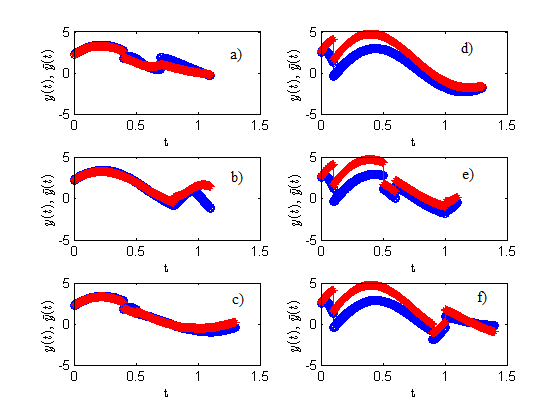
The procedure is also applied to get a reduced order approximation to an LSS whose local modes are unstable. The original LSS used in this case is an LSS of the form with , and . The resulting reduced order model is a -partial realization of of order . Note that the precise number of matched Markov parameters of the form is equal to the number of words in the set , and it is given by
The same parameters in the first example are used with the exception of minimum dwell time for both modes being and the simulation time horizon being . Again the output of the original system and the output of the reduced order system are simulated for random switching sequences and input trajectories. The mean of the BFRs for this example is ; whereas, the best acquired BFR is and the worst . The outputs and of the most successful simulation for this example are illustrated in Fig. 2.

VIII Conclusion
Two moment matching procedures for model reduction of continuous time LSSs has been given. The first method is the direct analogue of the moment matching approaches in the linear case, for LSSs. The second method relies on the nice selections of some desired vectors in the reachability or observability space of an LSS. The notion of nice selections gives flexibility to the user of the procedure in the following sense: It is possible to focus the approximation on some preferred local modes more than the others. It has been proven that with this procedure, as long as a certain criterion is satisfied, it is possible to acquire at least one reduced order approximation to the original LSS whose Markov parameters related to the specific nice selection are matched with the original one’s. Finally, it has been shown that nice selections can be used for matching the input - output behavior of an LSS with another one of possibly lower order, for a specific switching sequence. Discovering the relationship between a set of switching sequences with nice selections for continuous time LSSs would be a potential future research topic since it would solve the problem of approximation or minimization for restricted switching dynamics.
Appendix A Proof of Theorem 5
To present the proof of Theorem 5 we will introduce an ordering on as follows:
Definition 14.
(Ordering on ). Suppose that . Let the map be defined as follows:
| (34) | ||||
where , , . Then an ordering on the elements of can be defined as follows: For any two words , if , then .
Intuitively, this ordering states that if is bigger than when the words are interpreted as integer numbers in the basis . Note that for any , implies , and implies .
Proof of Theorem 5.
i) Let denote the matrix
where denotes the cardinality of the set ; and with respect to the ordering in Definition 14.
In this part of the proof, of is assumed to be zero for simplicity in notation, note that the proof can easily be modified for the case when is nonzero. Since is assumed to be minimal, for any , there exists linearly independent columns of . Suppose these columns are picked in the following manner: Scanning through the columns of from left to right, choose the first columns linearly independent from the preceding columns. Our claim is that, this method would yield a nice column selection. To prove the theorem, we claim that if is an element of the selection defined, must also be an element i.e., if , . We prove this claim by contradiction. Suppose the columns are chosen in this way and for a , and , the th column of is an element of this selection while the th column of is not. This means is a linear combination of the columns of preceding it while is not. Let denote the columns of which precede the column and with denote the columns of which precede the column . Note that for some
Thus the column can be written as
| (35) | ||||
and since all the vectors precede the column , each of them can also be written as a linear combination of the columns which precede . That means for some , , , (35) can be rewritten as
i.e., the column is a linear combination of its preceding columns. This contradicts our assumption and concludes the proof of the reachability part.
ii) This part is the dual of part i. ∎
References
- [1] A. C. Antoulas. Approximation of Large-Scale Dynamical Systems. SIAM, Philadelphia, PA, 2005.
- [2] A. Arnold, A. Vincent, and I. Walukiewicz. Games for synthesis of controllers with partial observation. Theoretical Computer Science, 303(1):7–34, June 2003.
- [3] Z. Bai and D. Skoogh. A projection method for model reduction of bilinear dynamical systems. Linear Algebra and its Applications, 415(2 - 3):406 – 425, 2006.
- [4] M. Bastug, M. Petreczky, R. Wisniewski, and J. Leth. Model reduction of linear switched systems by restricting discrete dynamics. In Accepted for publication in Proc. of the IEEE Conference on Decision and Control (CDC), Los Angeles, CA, USA.
- [5] M. Bastug, M. Petreczky, R. Wisniewski, and J. Leth. Model reduction by moment matching for linear switched systems. In Proc. of the American Control Conference (ACC), pages 3942 – 3947, Portland, OR, USA, June 2014.
- [6] A. Birouche, J Guilet, B. Mourillon, and M Basset. Gramian based approach to model order-reduction for discrete-time switched linear systems. In Proc. Mediterranean Conference on Control and Automation, 2010.
- [7] Y. Chahlaoui. Model reduction of hybrid switched systems. In Proceeding of the 4th Conference on Trends in Applied Mathematics in Tunisia, Algeria and Morocco, May 4-8, Kenitra, Morocco, 2009.
- [8] G. M. Flagg. Interpolation Methods for the Model Reduction of Bilinear Systems. PhD thesis, Virginia Polytechnic Institute, 2012.
- [9] H. Gao, J. Lam, and C. Wang. Model simplification for switched hybrid systems. Systems & Control Letters, 55:1015–1021, 2006.
- [10] E. Grädel, W. Thomas, and T. Wilke. Automata, Logic and Infinite Games, volume LNCS 2500. Springer, 2002.
- [11] S. Gugercin. Projection methods for model reduction of large-scale dynamical systems. PhD thesis, Rice Univ., Houston, TX, May 2003.
- [12] C.G.J.M. Habets and J. H. van Schuppen. Reduction of affine systems on polytopes. In International Symposium on Mathematical Theory of Networks and Systems, 2002.
- [13] M. Hazewinkel. Moduli and canonical forms for linear dynamical systems II: The topological case. Mathematical Systems Theory, 10:363–385, 1977.
- [14] G. Kotsalis, A. Megretski, and M. A. Dahleh. Balanced truncation for a class of stochastic jump linear systems and model reduction of hidden Markov models. IEEE Transactions on Automatic Control, 53(11), 2008.
- [15] G. Kotsalis and A. Rantzer. Balanced truncation for discrete-time Markov jump linear systems. IEEE Transactions on Automatic Control, 55(11), 2010.
- [16] O. Kupferman, P. Madhusudan, and P.S. Thiagarajan. Open systems in reactive environments: Control and synthesis. In CONCUR’00, 2000.
- [17] D. Liberzon. Switching in Systems and Control. Birkhäuser, Boston, MA, 2003.
- [18] Y. Lin, L. Bao, and Y. Wei. A model-order reduction method based on krylov subspaces for mimo bilinear dynamical systems. Journal of Applied Mathematics and Computing, 25(1-2):293–304, 2007.
- [19] L. Ljung. System Identification, Theory for the User. Prentice Hall, Englewood Cliffs, NJ, 1999.
- [20] E. Mazzi, A.S. Vincentelli, A. Balluchi, and A. Bicchi. Hybrid system model reduction. In IEEE International conference on Decision and Control, 2008.
- [21] N. Monshizadeh, H. Trentelman, and M. Camlibel. A simultaneous balanced truncation approach to model reduction of switched linear systems. Automatic Control, IEEE Transactions on, PP(99):1, 2012.
- [22] M. Petreczky. Realization theory for linear and bilinear switched systems: formal power series approach - part i: realization theory of linear switched systems. ESAIM Control, Optimization and Caluculus of Variations, 17:410–445, 2011.
- [23] M. Petreczky, P. Collins, D.A. van Beek, J.H. van Schuppen, and J.E. Rooda. Sampled-data control of hybrid systems with discrete inputs and outputs. In Proceedings of 3rd IFAC Conference on Analysis and Design of Hybrid Systems (ADHS09), 2009.
- [24] M. Petreczky and G. Mercère. Affine LPV systems: realization theory, input-output equations and relationship with linear switched systems. In Proceedings of the IEEE Conference on Decision and Control, Maui, Hawaii, USA, December 2012.
- [25] M. Petreczky and R. Peeters. Spaces of nonlinear and hybrid systems representable by recognizable formal power series. In Proc. 19th International Symposium on Mathematical Theory of Networks and Systems, pages 1051–1058, Budapest, Hungary, July 2010.
- [26] M. Petreczky and J. H. van Schuppen. Partial-realization theory for linear switched systems - a formal power series approach. Automatica, 47:2177––2184, October 2011.
- [27] M. Petreczky, R. Wisniewski, and J. Leth. Balanced truncation for linear switched systems. Nonlinear Analysis: Hybrid Systems, 10:4–20, November 2013.
- [28] H. Shaker and R. Wisniewski. Generalized gramian framework for model/controller order reduction of switched systems. International Journal of System Science, 42:1277––1291, August 2011.
- [29] Z. Sun and S. S. Ge. Switched linear systems : control and design. Springer, London, 2005.
- [30] P. Tabuada. Verification and Control of Hybrid Systems: A Symbolic Approach. Springer-Verlag, 2009.
- [31] R. Tóth, H. S. Abbas, and H. Werner. On the state-space realization of lpv input-output models: Practical approaches. IEEE Trans. Contr. Syst. Technol., 20:139–153, January 2012.
- [32]
W.M. Wonham.
Supervisory control of discrete-event systems.
Lecture notes,
http://www.control.utoronto.ca/~wonham. - [33] L. Zhang, E. Boukas, and P. Shi. Mu-dependent model reduction for uncertain discrete-time switched linear systems with average dwell time. International Journal of Control, 82(2):378– 388, 2009.
- [34] L. Zhang and P. Shi. Model reduction for switched lpv systems with average dwell time. IEEE Transactions on Automatic Control, 53:2443–2448, 2008.
- [35] L. Zhang, P. Shi, E. Boukas, and C. Wang. Model reduction for uncertain switched linear discrete-time systems. Automatica, 44(11):2944 – 2949, 2008.