Zero-dynamics principle for perfect quantum memory in linear networks
Abstract
In this paper, we study a general linear networked system that contains a tunable memory subsystem; that is, it is decoupled from an optical field for state transportation during the storage process, while it couples to the field during the writing or reading process. The input is given by a single photon state or a coherent state in a pulsed light field. We then completely and explicitly characterize the condition required on the pulse shape achieving the perfect state transfer from the light field to the memory subsystem. The key idea to obtain this result is the use of zero-dynamics principle, which in our case means that, for perfect state transfer, the output field during the writing process must be a vacuum. A useful interpretation of the result in terms of the transfer function is also given. Moreover, a four-nodes network composed of atomic ensembles is studied as an example, demonstrating how the input field state is transferred to the memory subsystem and how the input pulse shape to be engineered for perfect memory looks like.
1 Introduction
Quantum memory is, in a wide sense, a device that stores or freezes a quantum state both spatially and in time. A highly successful example is that a light pulse is frozen in a cloud of atoms [1, 2, 3, 4, 5]. Also quantum memory is of technological importance particularly in quantum information science, such as the quantum repeater for quantum communication [6, 7, 8]. Because of these scientific/technological importance, the field of quantum memory has experienced significant progress in both theory and experiment. We refer to for instance [9, 10, 11] for reviewing the current situation of this very active research area.
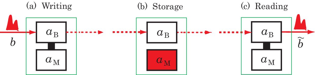
Now let us see a basic and general schematic of an ideal quantum memory in an abstract way. First of all, we assume that the system contains a subsystem that can store any quantum state without loss in a long period of time; we call this specific component the memory subsystem. Ideally, the memory subsystem should be completely decoupled from the other system components and surrounding environment during it stores the state; i.e., it is decoherence free (DF) [12, 13, 14, 15]. Note that, in this storage stage, the memory subsystem is decoupled even from the channel used for transferring an input state or retrieving the stored state. Hence, the second assumption is that, during the writing/reading process, the system can be tuned so that the memory subsystem couples to that transportation channel. That is, the system should be the one that contains a tunable port switching the opening/closing of the memory subsystem. Indeed this basic schematic is employed in each specific memory device. In the case of atoms based on the electromagnetic induced transparency (EIT) effect, an isolated memory subsystem is served by a set of metastable collective atomic states, and an external control field (with Rabi frequency ) can switch ON/OFF of the coupling between the metastable states and the optical field for state transportation [1, 2, 3, 4, 16, 17]. We also find successful demonstrations in optical cavity or optomechanical oscillator arrays [18, 19, 20, 21, 22], where the switching mechanism is served by adiabatic frequency detuning of the memory subsystem. Further, a similar switching procedure is employed in the photon echo quantum memory [10]. Note that, if the system does not contain a switching mechanism, it is generally impossible to perfectly transfer an unknown state to a memory subsystem (i.e. DF subsystem) [23].
The above-mentioned basic schematic for quantum memory is illustrated in Fig. 1. In the writing stage (a), an input state is sent to the system over an input channel with mode . Let us here assume that, by devising a “certain nice procedure”, all the input state is transferred to the memory subsystem with mode . We then close the port, and becomes decoherence free. In this storage stage (b), ideally, the memory subsystem can store the state for a long time. Finally, in the reading stage (c), by opening again the port we can retrieve the state at any later time, which is sent over the output channel with mode .
So what is a “certain nice procedure” to achieve the best or hopefully perfect state transfer? For some typical quantum memories such as EIT and off-resonant Raman memories, we can explicitly formulate this problem; that is, the question is what is the optimal temporal shape of the pulsed light field carrying the input state. This optimization problem is very important and actually has been deeply investigated in several papers; for instance, towards the most efficient atomic memory with EIT, in [24, 25, 26, 27] the input wave packet as well as the controllable Rabi frequency (see the second paragraph) are carefully designed, although the method is a heuristic one based on iterative tuning of the parameters. It is also notable that the so-called rising exponential type function is found as an effective pulse shape [28, 29, 30]. This is a pulse with exponential increase of e.g. the probability density of photon counting or the amplitude of a coherent field, which can be physically implemented [31, 32, 33]. Motivated by these results and further the fact that a large-scale quantum memory is required for constructing practical quantum communication architecture, the following questions naturally arise. Is there a pulse shape for achieving perfect state transfer for general and large-scale quantum memory networks? Is there a general yet simple guideline for synthesizing such desirable pulse shape? What is the fundamental origin of the rising exponential function as a desirable pulse shape? Is the rising exponential pulse optimal in a certain sense? Also, is it effective even for a large-scale network? Solving these problems should accelerate the progress of the quantum memory research in its deeper understanding and practical implementation.
In this paper, we consider a general passive linear system, which models a wide variety of systems such as optical systems [18, 19, 20, 22, 34, 35], nano-mechanical oscillators [21, 36, 37], vibration mode of a trapped particle [38, 39], and atomic ensembles [24, 25, 26, 27, 28, 29, 40, 41, 42, 43, 44, 45]. As mentioned before, the system is assumed to contain a tunable memory subsystem; that is, by tuning a certain parameter, we can switch opening/closing of the memory subsystem, which is DF during the storage period. Note that in our case this DF subsystem corresponds to a system having the so-called dark mode [46, 47]. Another assumption is that an unknown input state to be transferred is encoded in a continuos-mode single-photon field or a coherent field. With these setups, we give answers to all the questions posed in the above paragraph. The essential idea is the use of zero-dynamics principle. This concept originates from the classical notion of “zero” of a transfer function, which is a fundamental tool used in systems and control theory [48]. More precisely, for a general linear classical system
where is the input, is the output, and are matrices, its input-output relation is simply characterized by a transfer function as (see Section 4.3 for detailed description); then, if the input is given by , where is a zero of the transfer function (meaning ), we have under some additional conditions. That is, the zero-dynamics is a system whose output is always zero. In fact, the concept of zero-dynamics is very important in analysis and synthesis for even general nonlinear systems [49, 50].
Actually, the zero-dynamics principle described above can be directly applied to general quantum memory problem; if the state transfer is perfectly carried out, the input field must be completely absorbed in the system, and the output field must not contain any small pieces of the input field. That is, as a principle, the output should be “zero” during the writing and storage stages. Surprisingly, this simple zero-dynamics principle leads us to prove, very easily, that a rising exponential function is a unique pulse shape achieving the perfect state transfer for general (and thus large-scale) linear passive networks. Moreover, based on this first main result, we give an explicit, simple, and general procedure for designing the wave packet carrying an unknown state that is as a result perfectly absorbed in the memory subsystem.
This paper is organized as follows. Section 2 provides some preliminaries, describing general passive linear systems, optical field states, and linear DF subsystems. Also the problem is explicitly formulated in Section 2.4. In Section 3, we study a simple single-mode oscillator as a memory system, to show the fact that a rising exponential function appears as a unique pulse shape achieving the perfect state transfer; based on this result, the idea of zero-dynamics principle is discussed. Section 4 provides our first main result; for general passive linear systems, we derive the rising exponential pulse from the zero-dynamics principle. Also we give a useful interpretation of this fact in terms of the transfer function. In Section 5, we present our second main result, showing the concrete procedure for perfect writing, storage, and reading; this explicitly shows the pulse shape to be synthesized for perfect state transfer from the optical field to the memory subsystem. Section 6 is devoted to derive the time evolution equations of some statistical quantities of the dynamics, which is useful for numerical simulation. In Section 7, we study a linear network composed of atomic ensembles trapped in a cavity, which contains a tunable memory subsystem; this example shows how the designed pulse actually looks like and how the state transfer from the optical field to the atomic ensembles evolves in time. Section 8 summarize the paper and discusses some future works. In Appendix A, we briefly examine the case of an active linear memory system. Appendix B provides a case study comparing the zero-dynamics principle and the so-called dark state principle.
Notation: We use the following notations: for a matrix , the symbols , , and represent its Hermitian conjugate, transpose, and complex conjugation in elements of , respectively; i.e., , , and . For a matrix of operators we use the same notation, in which case denotes the adjoint to . For a time-dependent variable , we denote .
2 Preliminaries and problem formulation
2.1 Passive linear systems
In this paper, we study a general linear open system composed of oscillators with mode that couples to an optical field with continuous mode ; hence they satisfy and . The system is driven by a quadratic Hamiltonian with an -dimensional Hermitian matrix. The system and the field instantaneously couple through the interaction Hamiltonian with an -dimensional complex row vector. Then the unitary operator
| (1) |
( is the initial time) produces the Heisenberg equations of and as follows;
| (2) |
where and . The second term in stems from the Ito-correction. Note also that, due to the ideal Markov property, the optical field does not have its own dynamical time evolution; rather represents the output of the system.
The above open system with input and output is called the passive linear system in the sense that it does not contain any active component such as an optical parametric amplifier in optics case. As mentioned in Section 1, a passive linear system can model a wide variety of systems. The main reason why we focus on this class of general systems is that it preserves the total energy during the interaction between the system and the field. This implies that the perfect state transfer is equivalent to the perfect energy transfer, which as a result allows us to use the zero-dynamics principle to characterize the perfect memory; this will be discussed in detail in Section 4. Also in Appendix A, we show a brief case study where the system contains an active component. For a general treatment of passive linear systems, see [35, 51, 52]; the notation used in this paper follow these references, where in general is an complex matrix representing input optical fields.
2.2 Input field states
In this paper, we consider the case where the input is given by a single photon state or a coherent state, which is carried by an optical pulse field with continuous-mode . They are described as follows.
Single photon field state: The single photon state in a single mode system is, as is well known, produced by acting a creation operator to the ground state ; i.e.
To describe the continuous-mode single photon field state, we define the annihilation and creation process operators
| (3) |
is an associated function in , representing the shape of the optical pulse field. Also satisfies the normalization condition . Due to this, and satisfy the usual CCR; . The single photon field state is, in a similar way as above, produced by acting the creation process operator on the vacuum field as follows [53, 54, 55, 56, 57]:
| (4) |
Due to the normalization condition of , we find that . Also note the relation ; thus, has the meaning of the wave function with the probability of photo detection per unit time. Let us now assume that the pulse shape can be expanded as
| (5) |
The coefficient represents (unknown) classical information encoded in the optical field, which satisfies , and is a set of orthonormal functions satisfying
| (6) |
Note that is the number of modes of the system. Then the single photon field state (4) can be written as
| (7) |
is called the single photon code state with pulse shape [54]; from the condition (6), they are orthonormal, i.e. . Also the field operator satisfies the CCR .
Coherent field state: Another important state is a coherent state. A coherent state in a single mode system is generated by acting a displacement operator on the ground state as follows;
where denotes the amplitude of . Likewise, a coherent field state is defined in terms of the creation and annihilation process operators as follows;
where is a complex-valued function, representing the amplitude of the state; that is, this is a coherent pulse field modulated with envelope function . Note that is not necessarily normalized, but its power is finite. Now we assume that is given, in terms of the orthonormal functions , by
| (8) |
where represents (unknown) classical information to be stored. The power of , i.e. the mean photon number in unit time, is then given by . The coherent field state is as a result described by
| (9) |
Note that this is not a superposition of the coherent field states , unlike the single photon field state (7).
2.3 Decoherence-free subsystem as a memory
Let us reconsider the linear system (2), which is composed of oscillators. Note again that this is an open system with representing the environment field. Therefore, during the system works as a memory, ideally some of its component, the memory subsystem with mode , must be decoupled from the field ; this means that the memory subsystem is exactly a decoherence-free subsystem [12, 13, 14, 15]. But the other component, the buffer subsystem with mode , still couples to . In contrast to , the state of the buffer subsystem decoheres due to the coupling to . As a result, in the storage stage, the dynamical equation of the system, Eq. (2), should be of the form
| (10) |
This equation clearly shows that is decoherence free, and its state is preserved. Note that does not appear in the output equation, implying that the energy contained in the memory subsystem does not leak out into the field.
The general theory of DF subsystems states that, if a DF subsystem exists, then the system Hilbert space is decomposed to , where any observable in evolves unitarily. In our case, the decomposition is of the form ; thus the system variables are, more precisely, represented by and . This special class of continuous-variable DF subsystems appears in several situation [46, 47, 58, 59, 60]. Also for a general theory of the linear DF subsystem, including a necessary and sufficient condition for a given linear system to have a DF mode, see [61].
2.4 Problem description
Here we describe the problem discussed throughout the paper.
Our system is the general passive linear system (2), and it is assumed to be tunable; that is, by appropriate tuning of its parameter(s), a part of the system, the memory subsystem, couples or decouples to the optical field carrying the information. Hence the memory subsystem can be switched to be a DF or a non-DF subsystem. As mentioned in Section 2.3, the memory subsystem stores the state during it is in the DF mode, while it should be in the non-DF mode when we transfer the input state or retrieve the stored state. In particular, we assume that the matrix in the writing/reading stages is Hurwitz, i.e., the real parts of all the eigenvalues of are negative; as will be shown later, this condition is necessary for perfect state transfer. On the other hand, in the storage stage, the dynamical equation takes the form (10), thus is not Hurwitz.
The field’s initial state is given by in the case of single photon input field or in the case of coherent input field. The system’s initial state is assumed to be separable, hence it is given by . In particular, we will set it to be the ground state satisfying .
At time , the system and the field start to interact, via the unitary operator given in Eq. (1). The composite state at time is then given by or . In this writing stage, the memory subsystem is in the non-DF mode, so it couples to the field. But once the state transfer has been completed, then we switch the system parameters so that the memory subsystem becomes decoherence free, and its state is preserved during the storage stage. Hence, it would be desirable if the state is of the separable form
and the memory subsystem’s state contains the full information of the input field state or . Therefore, our goal is to appropriately synthesize the pulse shape or , or more precisely their basis functions , so that the above desirable transition from the field’s initial state to occurs.
Lastly we remark on the switching configuration. In general, the system matrices and (and thus ) can change in time (i.e. time varying) in order to realize high quality quantum memory. For instance in [24, 25, 26, 27], the authors consider the time varying system matrices depending on the control field with frequency , which is optimized via a heuristic method. On the other hand, in this paper, we assume that and are time varying, but they are constant in each stage of the memory procedure; that is, they are piecewise constant. In particular, we will take the same system matrices in the writing and reading stages.
3 Perfect state transfer in a single-mode passive linear system
In this section, we examine a simple case where the memory system is given by a single-mode passive linear system. As will be shown later, this system does not contain a tunable DF component, so it does not work as a perfect storage device. Rather the purpose here is that, by focusing only on the writing stage, requiring perfect state transfer uniquely determines the pulse shape of the input optical field. Based on this result, we then derive the explicit form of the output field, and show the notion of zero-dynamics in this case. Here we study only the single-photon input case, but it is straightforward to obtain a similar result in the case of coherent field state.
3.1 Pulse shaping for perfect state transfer
Let us consider the following single-mode (i.e. ) linear system interacting with an optical field, which is obtained by setting and in Eq. (2):
| (11) |
where is the interaction strength; in optics case, this system is typically given by an optical cavity with proportional to the transmissivity of the coupling mirror. The goal is to send a single photon state over the input pulse field and write it perfectly down to the system. Note that, however, clearly this system does not contain a tunable DF component, hence our interest here is only in the state transfer.
The input state is given by Eq. (7), which is now essentially . Thus in this case let us take a superposition of the vacuum and the single photon field state
where are the encoded (unknown) classical information. Recall that the system’s initial state is set to the ground state .
The dynamical equation (11) has the following solution:
where is the time we stop the interaction. This can be rewritten as
| (12) |
where
Note that . Equation (12) can be further represented as
| (13) |
is the field creation operator with pulse shape , which is defined in Eq. (3), and is the unitary operator given in Eq. (1). From the above equation we find that, in the limit , the field creation operator is completely mapped to the system creation operator . This means that the perfect state transfer from the optical pulse field to the system mode can be carried out as shown below. In the Schrödinger picture, the whole state at time is given by
where in the last equality is used. Let us now set the input pulse shape to be . Then, from Eq. (13), we have
Therefore, in the limit , we have
which means that the input field state is completely transferred to the system state. In particular, in the case and , the input pulse shape is given by
| (14) |
This is called the rising exponential pulse [24, 28, 29, 30, 31, 32, 33]. It is clear from the above discussion that the rising exponential is the unique pulse shape for perfect state transfer from the single photon field to the system.
3.2 Explicit form of the output field
Let us further study the final state , where the input pulse shape is now set to
| (15) |
It is possible to obtain the explicit solution:
where
with
First, at , we have
which becomes only when . That is, the frequency bandwidth of the input pulse shape has to be exactly equal to that of the memory system to attain the perfect state transfer. This is a form of the so-called impedance matching for efficient energy transfer; in Section 7, we will discuss the matching condition in a more practical setup where the system is composed of a cavity and atomic ensembles.
Next, in the limit , the whole state again becomes separable:
where
This represents the pulse shape of the output optical field over the whole period. Hence, if , the output field is vacuum in the writing stage ; this means that the single photon input field is completely absorbed into the system, and the output field does not contain any pieces of the input state. In the optics case where the system is given by a cavity, a physical meaning of this fact is that it happens destructive interference between the light field reflected at the coupling mirror and the transmissive light field leaking from the cavity; as a result, the output field of the cavity is always in vacuum, i.e. “zero”, while the system’s state still dynamically changes in time. In general, the dynamics of a system whose output is always zero is called the zero dynamics [48, 49, 50]. Hence in this case the cavity dynamics during the writing process is exactly a zero dynamics.
4 Zero-dynamics principle for perfect state transfer
In this section, based on the so-called energy-balanced identity, we show the notion of zero-dynamics principle as a guideline for perfect state transfer in general passive linear systems. Then, we prove that the zero-dynamics principle readily leads to the rising exponential function as a unique pulse shape. Further, a useful view of the zero-dynamics principle in terms of the transfer function is provided.
Note that the zero-dynamics principle is essentially equivalent to the so-called dark state principle; this idea was first employed in [62] for the application to a lossless node-to-node state transfer in a cavity QED network, and later several applications have been developed, e.g. lossless gate operation [63]. Appendix B provides a detailed case study comparing the zero-dynamics principle and the dark state principle and then discusses their difference.
4.1 Input-output relation of the pulse shape
First we remark that the pulse shape of the single-photon input field, , and that of the output field, say , can be connected through a dynamical equation having the same form as Eq. (2). Actually, by multiplying by Eq. (2) from the right hand side and using the relation , we find that the mean photon number of the output field is given by
By definition this should be written as , hence and are related through the following dynamics:
| (16) |
where is a -dimensional c-number vector. Note that does not have a particular physical meaning, unlike the vector appearing just below.
The same classical dynamical equation holds for the case of coherent input field; noting that , we readily see that the vector of mean amplitudes, with , follows
| (17) |
where is the amplitude of the output field . This equation has the same form as Eq. (16), hence in what follows we use Eq. (16) when discussing the input-output relation of the corresponding wave packets.
4.2 The zero-dynamics principle and rising exponential pulse
To pose the zero-dynamics principle, it is important to first remember that, for the general passive linear system (2), the following energy balance identity [64] holds:
| (18) |
This indicates that the total energy contained in the system and the field is preserved for all time. Indeed, from Eq. (18) we immediately have
where the mean is taken for the state . Now we assume . Then, for the energy of the input pulse field to be completely transferred to the system, we need for with the stopping time of the writing process. This is a rigorous description, in the case of passive linear systems, of the zero-dynamics principle; that is, for the general quantum memory problem with a passive system, the output field must be vacuum (i.e. “zero”) for perfect state transfer. Surprisingly, this simple condition uniquely determines the form of the input pulse shape as shown below.
First, from the requirement , we have , which further leads to
| (19) |
This has the solution , with a fixed vector. Thus, again from the condition , we have
Note that the input is sent during the writing stage , and in the storage and reading stages in . Taking this into account, we end up with the expression
| (20) |
where is the Heaviside step function taking for and for . Since is Hurwitz, as assumed in Section 2.4, the real parts of all the eigenvalues of are strictly positive. Hence Eq. (20) is a generalization of the rising exponential function. In fact, this immediately recovers the result (14) in the example, where , , and particularly . Lastly we remark that the zero dynamics is given by Eq. (19), which is defined up to time .
4.3 Transfer function approach
Let us define the (two sided) Laplace transform of a signal by
Note that, when , this represents the Fourier transformation. Then the Laplace transformation of Eq. (16) gives
| (21) |
The transfer function characterizes the input-output relation of the linear system (16) in the Laplace domain. As explained in Section 1, the zero-dynamics principle originates from the classical notion of “zero” of a transfer function [48], and we can now explicitly describe this fact.
First, to see the idea let us return to the example studied in Section 3. The input pulse shape is given by Eq. (14), whose Laplace transformation is . Also in this case the transfer function is given by
| (22) |
Hence, the output is computed as
and its inverse Laplace transform then yields
Thus, we again see that the input field is completely absorbed in the system during ; i.e. the perfect state transfer has been carried out. The most notable point is clearly that the zero of is erased (in general, if for a transfer function there exists a satisfying , then is called a zero).
Now we can generalize the above fact; for simplicity, we set . The transfer function of the general passive linear system is given by Eq. (21). Also the Laplace transformation of the rising exponential function (20) is given by
Therefore, the output is computed as
Since is Hurwitz, the output does not contain a zero, implying .
In general, if a transfer function contains a (transmission) zero, then there alway exists an input signal such that the corresponding output takes zero [48]. Therefore, we have the following interpretation of the zero-dynamics principle for quantum memory in terms of transfer function; in general, a linear memory system needs to have a zero for perfect state transfer, and the input state is sent over an optical field whose pulse shape is characterized by that zero. This view would be useful particularly in the case of multi input channels.
5 Perfect memory procedure in passive linear system
In this section, we provide a detailed procedure to achieve the perfect memory, which is composed of the following three stages; the perfect state transfer from the input field to the memory subsystem (writing), decoherence-free preservation of the transferred state (storage), and the appropriate retrieving of the system state into the output field (reading). The setup was described in Section 2.4; note again that the system matrices and (thus ) change depending on the memory stage, but they are piecewise constant. Also, as motivated by the result obtained in Section 3, we will take , while keeping general .
One of the main questions is as follows; although we have derived the rising exponential function (20) from the zero-dynamics principle, it still contains some parameters that should be chosen appropriately; more precisely, it is given by , and we need to determine so that the input field state is completely transferred to the memory subsystem. In this section, we will see that this synthesis problem is clearly solved.
5.1 The writing stage
The solution of the general linear equation (2) is explicitly given by
Since is Hurwitz, we can take the limit , which yields
where again is the stopping time of the writing process. Let us now define the following vector of rising exponential functions:
| (23) |
Then the above solution of can be expressed as
This is a vector of creation operators , implying that it has to satisfy the canonical commutation relation ; actually, we have
This relation shows that are orthonormal; .
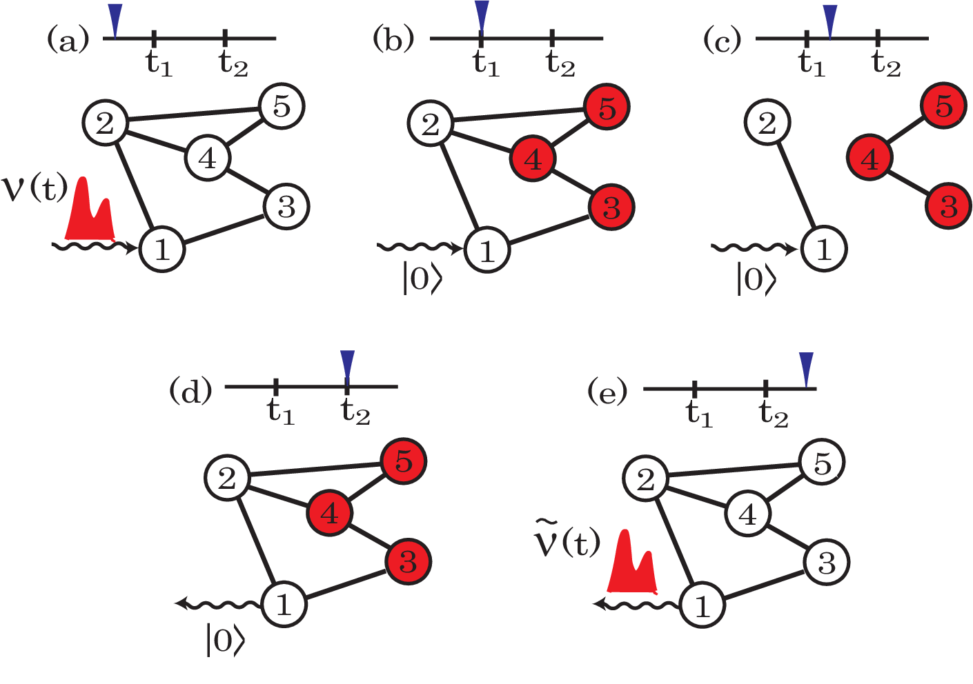
Case I: Single photon state. We consider the case where the input is the single photon field state (7). Also the system is assumed to be in the separable ground state at the initial time . Then, through the interaction (see Fig. 2 (a)) the whole state changes to
where denotes the unitary time evolution (1). We here set the basis functions to the rising exponential functions given in Eq. (23), meaning that the input pulse shape (5) is chosen as
| (24) |
Then, noting that , we obtain
| (25) |
where with appearing only in the th entry. Therefore, through the interaction, at time the system completely acquires the input code state with coefficient ; the resulting system state is highly entangled among the nodes (see Fig. 2 (b)). The optimal input pulse shape is given by the rising exponential function of the form (20), as expected in Section 4.2. But the point here is that we now know that the parameter vector in Eq. (20) exactly corresponds to the superposition coefficients . Together with the structure of the memory subsystem, this fact tells us how we should design the input pulse shape ; this will be more precisely discussed in the next subsection.
Case II: Coherent state. Next, let us consider the case where the input is the coherent field state (9). Again the system is in the ground state at . Then, through the interaction the whole state becomes
Therefore, by setting the basis functions to the rising exponential (23) i.e.
| (26) |
and again noting that , we obtain
| (27) |
That is, the system state is changed to the product of coherent states . Hence, similar to the single photon case, the perfect state transfer is possible by sending the information over the rising exponential pulse field.
5.2 The storage stage
As mentioned in Sections 1 and 2.4, the key architecture of an ideal memory device is that the system contains the tunable memory subsystem that can be switched to DF mode in the storage stage or non-DF mode in the other two stages; now we are in the storage stage. Especially to describe the idea explicitly, let us consider the case only in this subsection and assume that, after the writing process has been completed at time , the system can be immediately switched so that its dynamical equation is of the following form:
where is the buffer mode and is the memory mode. Clearly, constitutes a DF subsystem. Hence, in the single photon input case, the whole state cannot be preserved, but only its (3, 4, 5) components can be. This means that the original field state with can be perfectly transferred and stored in the memory subsystem; hence the input pulse shape should be synthesized by multiplying the classical information with the basis functions , generating as a result . Indeed, in this case, the whole state just after the writing process is given by
and thus the state is preserved; see Fig. 2 (c).
The idea is the same for the coherent input case. That is, the state
can be perfectly transferred and stored in the memory subsystem.
5.3 The reading stage
Suppose that the state has been perfectly stored during the period ; hence the reading stage starts at time with the initial state for the single photon input case or for the coherent input case; see Fig. 2 (d). Note that, as described in Section 5.2, only some elements of or , which represents the classical information of the stored state, are not zero. To retrieve this initial state, we switch the system matrices so that the memory subsystem again couples to the buffer subsystem and thus the optical field; in particular, we take the same system matrices and (and thus ) as in the writing stage. Thus note that is Hurwitz.
To describe the reading stage, first, we particularly focus on the following quantity:
The first term is . For the second and the third terms, by defining , which leads to , we find that they become
As a result, we have
| (28) |
where
| (29) |
As in the previous case, are orthonormal; . Note that is a generalization of a decaying exponential function. Moreover, Eq. (28) leads to
Case I: Single photon state. The initial state is now . Then, through the interaction, this state changes to:
Therefore, certainly the field state recovers the input state (7), which is now carried by the output field with pulse shape (29). The system state returns to the ground state; see Fig. 2 (d,e).
Case II: Coherent state. The initial state is . Then, through the interaction, this state changes to:
where is a coherent field state with pulse shape
Thus, similar to the single photon input case, the stored coherent states leaks into the output field with pulse shape (29), and we can retrieve the full information about contained in the coherent field state .
6 Statistical equations in the writing stage
Here we derive the time evolution equations of the statistics in the writing stage. These equations are useful for numerical simulation, as demonstrated in the next section.
Case I: Single photon state. In the case of single photon state, we evaluate the following matrix of operators:
The photon is distributed in the system according to the statistics represented by the correlation matrix . The time-evolution equation of is, together with the vector , given by
| (30) | |||
| (31) |
The solution of Eq. (31) is readily obtained as
where is used. In general, the Lyapunov differential equation , with time varying, has the solution of the form
If is Hurwitz, in the limit of , this becomes
Using this result and the expression (23), we have
If we send the single photon code state over the input field with rising exponential pulse shape , then we have due to . This means that the input single photon state is distributed among the network so that the th node has the mean photon number at time .
Case II: Coherent state. In this case the statistics is more convenient, because a coherent state is completely charactered only by its mean and variance. In particular, the dynamics of the mean, , was already obtained in Eq. (17), with particularly given by in Eq. (26). Hence it is immediate to obtain the solution in :
Hence, by taking the limit , we have ; i.e. . Also, we evaluate the covariance matrix with , which takes zero if and only if the state is a coherent state. Similar to the single photon case, we find that obeys , which readily yields as . As a result, the th node becomes the coherent state at time . We note that the mean of the output field is for all ; thus the zero-dynamics principle is certainly satisfied.
7 Example: Perfect memory network with atomic ensembles
This section is devoted to study a passive linear network composed of atomic ensembles, which contains a tunable DF component. A numerical simulation will demonstrate how the input field state is transferred to the memory subsystem and how the input pulse shape to be engineered for perfect memory looks like.
7.1 The atomic ensembles trapped in a cavity

The system is three large atomic ensembles trapped in a single-mode cavity, depicted in Fig. 3; a detailed description of this system is found in e.g. [40, 41, 42, 43, 44, 45]. The annihilation operator represents the cavity mode, and is the annihilation operator approximating the collective lowering operator of the th ensemble. The internal cavity light field and the th ensemble interact with each other through external pulse lasers with Rabi frequencies and . The coupling Hamiltonian is given by
| (32) |
where is the laser phase, is the number of atoms in each ensemble, is the coupling strength, and is the detuning. The spontaneous emission of each atom is negligible for typical atoms such as 87Rb. We also assume that the second and third ensembles can be manipulated via external magnetic fields, which introduce the self Hamiltonian with denoting the tunable strength of the magnetic field. We here set the parameters as and for , and define ; then, the total system Hamiltonian is given by
The cavity field couples to an external optical field with continuous mode used for state transfer, at the beam splitter with transmissivity proportional to ; this means that the system-field coupling Hamiltonian , which was defined above Eq. (1), is specified with . Consequently, the system matrices are given by
Note that this passive linear system can be physically realized in some other systems, such as a mechanical oscillator array connected in a single mode cavity.
7.2 The perfect memory procedure
We can prove that, when , the matrix is Hurwitz; i.e. the real part of all the eigenvalues of is negative. A convenient way to see this fact is to use the property that the controllability matrix is of full rank iff is Hurwitz [52]. Thus the system does not contain a DF component when . On the other hand, if we turn off the magnetic field and set , then a DF subsystem appears, as shown below. Let us take the following unitary matrix:
This transforms the system equation to
where
| (52) |
Therefore, when , the system takes a form of Eq. (10). That is, is not affected by the incoming field and it does not appear in the output field ; hence is the memory subsystem that can be switched to a DF or non-DF subsystem, just by controlling the external magnetic field. This two-mode subsystem works as a perfect memory that preserves any state of the form in the case of single photon state or in the case of coherent state. Note that and depend on the atomic modes and not on the cavity mode , implying that the state is indeed stored in the atomic ensembles. Also it should be remarked that and take the form of continuous-variable syndromes used for quantum error correction [65, 66].
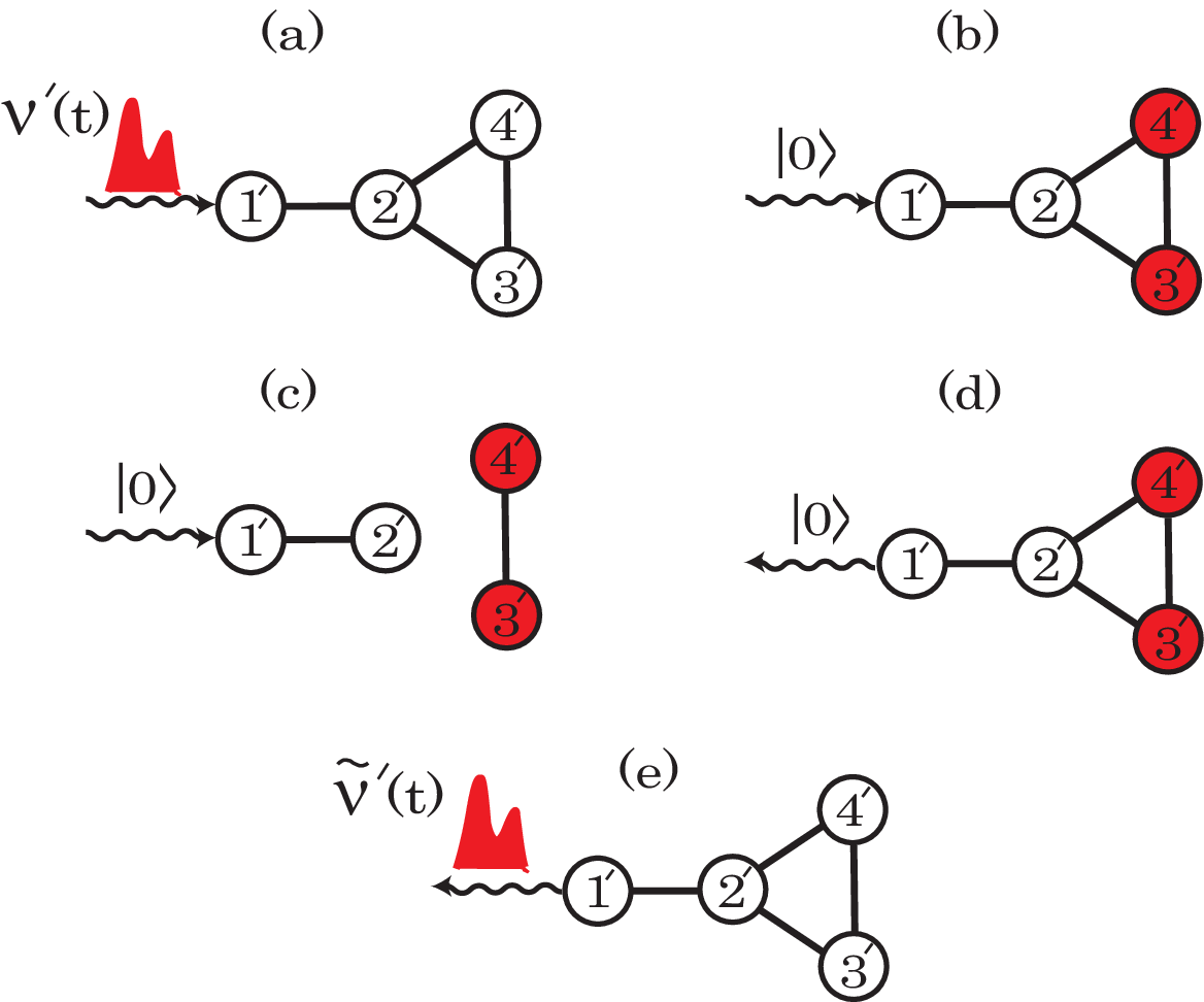
Here we describe the concrete procedure of the writing, storage, and reading processes, in the case of single photon input; see Fig. 4.
- •
A single photon field state is prepared in the form , where and are the third and fourth elements of the vector of rising exponential functions with and given in Eq. (7.2). Note in this stage the magnetic field is ON; .
- •
The field couples to the system until . The perfect state transfer is achieved in the end, at , by sending the input state over the optical field with pulse shape described above. The whole state changes to .
- •
We turn off the magnetic field and set ; then the memory subsystem with modes becomes decoherence free and its state is preserved during an arbitrary time interval .
- •
At a later time , we turn on the magnetic field (i.e. set ) to retrieve the stored state. Then the memory subsystem again couples to the optical field, and the perfect copy appears in the output field with the pulse shape specified by .
Recall that the optimal input pulse shape is determined by the properties (zeros) of the memory system and this corresponds to the impedance matching mentioned in Section 3.2. Now we should note that an additional matching condition is not imposed on the interaction between the cavity mode and the atomic ensembles, although perfect state transfer from the former to the latter is certainly achieved. This result seems to be inconsistent with the fact obtained in [68, 69, 70, 71], showing that perfect state transfer from a cavity to an inhomogeneously broadened (IB) atomic ensemble requires a strict impedance matching between them. But there is a clear difference between our case and those studies; in the case dealing with the IB ensemble, due to the matching condition, an input field state with arbitrary (yet within a finite band-width) temporal shape is allowed to be completely absorbed into the ensemble (see e.g. [10, 72] for the recent experimental results), while in our case the optimal pulse shape has to be strictly specified. Exploring a combined schematic of these two memory procedures, which would allow weaker pulse shaping and weaker impedance matching, should be an interesting future work.
7.3 Numerical simulation

Here we demonstrate a numerical simulation of the writing stage of the above memory procedure. The parameters are set to , , and ; note again in this stage and there is no DF subsystem. The input is a single photon field state with coefficients , which is carried by the optical field with pulse shape and as mentioned above. The initial time is and the stopping time is .
First, Fig. 5 (a) shows the absolute value of and . These are the pulse shapes we need to correctly engineer for the desirable perfect state transfer. A notable point is that they are not anymore of a rising exponential shape such as Eq. (14); particularly they take the value zero at the stopping time . A similar non-rising exponential pulse function was also found in [67], achieving perfect state transfer in an integrated quantum memory system. It looks that we can realize this kind of pulse shape by combining some Gaussian wave packets, which might be a desirable feature from the engineering viewpoint.
Next, Fig. 5 (b) shows the time-evolutions of the mean photon number of each node, i.e. , which can be computed by numerically solving Eqs. (30) and (31). As expected from the theory, the memory subsystem with modes perfectly acquires the photon with mean photon number at . We should note that the transportation of the photon from the input field to the memory subsystem occurs rapidly only in the last few period; in fact, almost all the energy contained in the input pulses and is confined in this short period. Hence, we need to be very careful to stop the writing process at the accurate time , because the desired state is fragile in the following sense. For instance if we turn off the magnetic field a bit earlier than , say , then the whole system’s state generated is roughly (unnormalized); thus the state of the memory subsystem becomes a mixed state (unnormalized)
due to the decoherence added to the buffer subsystem with modes during the storage period. Hence, an important future work is to find a suitable set of parameters so that the time-evolutions of the mean photon numbers of the memory subsystem become as flat as possible at the stopping time .
8 Conclusion
In this paper, for a general passive linear system, we have provided a designing method of input pulse shape that perfectly transports a single photon or coherent field state to a memory subsystem, which can be switched to a DF subsystem. The method is general and simple, so it can be directly applied to a large-scale network; in fact, in the example studied in Section 7, we found that the explicit form of and are readily obtained. The results are based on the zero-dynamics principle. Although in this paper this principle was used only for synthesizing the input pulse shape, it is indeed a wide concept that works in a more general situation. For example, the zero-dynamics principle can be applied to the case where, instead of pulse shaping of the input field, some time-varying controllable parameters of the system should be engineered due to practical limitation; also the system can be nonlinear; further, we could deal with an inhomogeneously broadened atomic ensemble memory that allows an arbitrary temporal shape for perfect state transfer, which was discussed in Section 7.2. In any case, following the zero-dynamics principle, we should design the system so that the output is zero or more generally the output is minimized. Moreover, the zero-dynamics corresponds to the time-evolution of a state free from any energy loss, thus it represents a coherent, yet non-unitary, gate operation on the system state for quantum information processing; that is, designing a desired manipulation of a state in an open system is no more than designing a desired zero-dynamics. All these problems will be addressed in future works.
Appendix A Active memory system
In this paper, we thoroughly study a passive linear system, but there are many systems containing an active component. In general, for such an active system the energy balance identity (18) does not hold, hence the zero-dynamics principle does not anymore mean the perfect energy transfer. Hence, it should be worth doing a case study to see if an active system could allow perfect state transfer.
Let us consider the following active system:
In optics, this represents the dynamics of an optical parametric oscillator, where denotes the squeezing strength [34, 35]. Note that the system becomes passive if . The above equation can be explicitly solved:
Unlike the passive case, the field annihilation operator appears in the equation. Then under the same setting taken in Section 3 where the input field state is given by a superposition of the vacuum and with the pulse shape function given below, we obtain ( and )
where
This equation implies that, when , the perfect state transfer is impossible due to the third term, which clearly stems from the active element of the system. To carry out efficient state transfer, we need some approximation; in the above case, if is much bigger than , then the system state becomes approximately the desired one to be stored. Another example is found in [28], where the system is an atomic ensemble containing an active component, but by introducing a fast oscillating magnetic field it is approximated by a passive one, which was further shown to be a perfect memory.
Appendix B Dark state principle
The basic idea of dark state principle is as follows. For a system coupled to a probe field, we continuously monitor the system by a photo detector measuring the output field; then if the detector counts no photon, this means that the system is in a dark state and has a time evolution without loss of energy. Here we apply this dark state principle to the writing problem discussed in Section 3 and derive the same result; that is, in this sense, the zero-dynamics principle and the dark state principle are equivalent, though there is a big difference in practice as shown below.
First let us consider the case where we want to send a coherent field state to the system. In general, if we use a photon counter to estimate the system observables, our state (knowledge) conditioned on the measurement results is updated by the following stochastic master equation [73, 74] (the scattering operator is now set to be the identity):
where
is the pulse shape of the input coherent light field and is the measurement result (0 or 1) obtained during the small time interval . Also and are the system operators. Now since the ensemble averaging over the measurement results leads to a standard master equation, we have . Then, the counting probability of the measurement result “1” during is given by . Hence if , the system is in a dark state and loses no energy into the output field; the state satisfying this condition is called the dark state. In our case where the system is the single-mode passive linear system with and , the dark state can be specified to a coherent state because we now know that the system’s state is always a coherent state. The condition then becomes , which yields . Now, under the dark state condition the time evolution of the conditional state is identical to that of the averaged one, which consequently leads to . These two equations yield , thus the input pulse shape must be a rising exponential function .
Next let us consider the case where the input is a single photon field state. As in the above case, the dark state principle is represented in terms of the conditional state subjected to the single-photon stochastic master equation; see Eq. (43) in [74]. In this case the probability to obtain the measurement result “1” during is given by
where is the temporal pulse shape of the single photon field. are the operators characterizing the conditional state. Under the dark state condition , they obey
and , which are identical to the single-photon master equation [53]. The initial conditions are and . In our case and , these differential equations can be explicitly solved, yielding , , and , where and satisfy and . Substituting these solutions for the dark state condition , we have . Combining these three equations, we end up with the relation and thus see that the input pulse shape has to be a rising exponential function .
Summarizing, we have recovered the same result obtained in Section 3, showing that the dark state principle is equivalent to the zero-dynamics principle. Both principles require no energy leaking from the system into the output field, but their approaches are different; the dark state principle is represented in the Schrödinger picture, while the Heisenberg picture is used to describe the zero-dynamics principle. As a result, in the former case we need to solve the master equation, which is sometimes a hard task as demonstrated above especially in the single photon field case. On the other hand, we have seen in Section 4.2 that the zero-dynamics principle allows us to derive the rising exponential function very easily, even in the general setup; also the transfer-function-based treatment of the principle is notable and possibly very useful from the viewpoint of the applicability of the linear response theory to quantum memory. Of course these special advantages appear particularly in the linear case, and for more general nonlinear memory systems we should be careful in choosing the approach.
References
References
- [1] D. F. Phillips, A. Fleischhauer, A. Mair, R. L. Walsworth, and M. D. Lukin, Storage of Light in Atomic Vapor, Phys. Rev. Lett. 86, 783 (2001).
- [2] C. Liu, Z. Dutton, C. H. Behroozi, and L. V. Hau, Observation of coherent optical information storage in an atomic medium using halted light pulses, Nature 409, 25, 2001.
- [3] B. Julsgaard, J. Sherson, J. I. Cirac, J. Fiurasek, and E. S. Polzik, Experimental demonstration of quantum memory for light, Nature 432, 482, 2004.
- [4] T. Chaneliere, D. N. Matsukevich, S. D. Jenkins, S.-Y. Lan, T. A. B. Kennedy, and A. Kuzmich, Storage and retrieval of single photons transmitted between remote quantum memories, Nature 438, 833/836, 2005.
- [5] M. Hedges, J. Longdell, Y. Li, and M. Sellars, Efficient quantum memory for light, Nature 465, 1052/1056, 2010.
- [6] H. J. Briegel, W. Dur, J. I. Cirac, and P. Zoller, Quantum repeaters: The role of imperfect local operations in quantum communication, Phys. Rev. Lett. 81, 26, 1998.
- [7] L. M. Duan, M. D. Lukin, J. I. Cirac, and P. Zoller, Long-distance quantum communication with atomic ensembles and linear optics, Nature 414, 6862, 413/418, 2001.
- [8] N. Sangouard, C. Simon, H. de Riedmatten, and N. Gisin, Quantum repeaters based on atomic ensembles and linear optics, Rev. Mod. Phys. 83, 1, 2011.
- [9] A. I. Lvovsky, B. C. Sanders, and W. Tittel, Optical quantum memory, Nature Photonics 3, 706, 2009.
- [10] Special issue on quantum memory, Ed. by J.-L. Le Gouet and S. A. Moiseev, J. Phys. B: At. Mol. Opt. Phys. 45, 2012.
- [11] Focus on quantum memory, Ed. by G. Brennen, E. Giacobino, and C. Simon, New J. Phys. 2013.
- [12] A. Beige, D. Braun, and P. L. Knight, Driving atoms into decoherence-free states, New J. Phys. 2, 22, 2000.
- [13] D. Kielpinski, V. Meyer, M. A. Rowe, C. A. Sackett, W. M. Itano, C. Monroe, and D. J. Wineland, A decoherence-free quantum memory using trapped ions, Science 291, 1013, 2001.
- [14] D. A. Lidar and K. B. Whaley, Decoherence-free subspaces and subsystems, Irreversible Quantum Dynamics, edited by F. Benatti and R. Floreanini, Lecture Notes in Physics 622, 83, Springer Berlin/Heidelberg, 2003.
- [15] D. Bacon, Operator quantum error-correcting subsystems for self-correcting quantum memories, Phys. Rev. A 73, 012340, 2006.
- [16] M. Fleischhauer and M. D. Lukin, Quantum memory for photons: Dark-state polaritons, Phys. Rev. A 65, 022314, 2002.
- [17] Y.-H. Chen, et. al., Coherent optical memory with high storage efficiency and large fractional delay, Phys. Rev. Lett. 110, 083601, 2013.
- [18] Q. Xu, P. Dong, and M. Lipson, Breaking the delay-bandwidth limit in a photonic structure, Nature Physics 3 406, 2007.
- [19] Y. Tanaka, J. Upham, T. Nagashima, T. Sugiya, T. Asano, and S. Noda, Dynamic control of the Q factor in a photonic crystal nanocavity, Nature Mater. 6, 862, 2007.
- [20] A. W. Elshaari, A. Aboketaf, and S. F. Preble, Controlled storage of light in silicon cavities, Opt. Express 18-3, 3014, 2010.
- [21] D. E. Chang, A. H. Safavi-Naeini, M. Hafezi, and O. Painter, Slowing and stopping light using an optomechanical crystal array, New J. Phys. 13, 023003, 2011.
- [22] J. Yoshikawa, K. Makino, S. Kurata, P. van Loock, and A. Furusawa, Creation, storage, and on-demand release of optical quantum states with a negative Wigner function, Phys. Rev. X 3, 041028, 2013.
- [23] D. Kielpinski, R. A. Briggs, and H. M. Wiseman, Unavoidable decoherence in the quantum control of an unknown state, Q. Meas. and Q. Metrology 1, 1, 2013.
- [24] A. V. Gorshkov, A. Andre, M. D. Lukin, and A. S. Sorensen, Photon storage in Lambda-type optically dense atomic media, I. Cavity model, Phys. Rev. A 76, 033804, 2007; II. Free-space model, Phys. Rev. A 76, 033805, 2007; III. Effects of inhomogeneous broadening, Phys. Rev. A 76, 033806, 2007.
- [25] I. Novikova, A. V. Gorshkov, D. F. Phillips, A. S. Sorensen, M. D. Lukin, and R. L. Walsworth, Optimal control of light pulse storage and retrieval, Phys. Rev. Lett. 98, 243602, 2007.
- [26] I. Novikova, N. B. Phillips, and A. V. Gorshkov, Optimal light storage with full pulse-shape control, Phys. Rev. A 78, 021802, 2008.
- [27] N. B. Phillips, A. V. Gorshkov, and I. Novikova, Optimal light storage in atomic vapor, Phys. Rev. A 78, 023801, 2008.
- [28] C. A. Muschik, K. Hammerer, E. S. Polzik, and J. I. Cirac, Efficient quantum memory and entanglement between light and an atomic ensemble using magnetic field, Phys. Rev. A 73, 062329, 2006.
- [29] Q. Y. He, M. D. Reid, E. Giacobino, J. Cviklinski, and P. D. Drummond, Dynamical oscillator-cavity model for quantum memories, Phys. Rev. A 79, 022310, 2009.
- [30] Y. Wang, J. Minar, G. Hetet, and V. Scarani, Quantum memory with a single two-level atom in a half cavity, Phys. Rev. A 85, 013823, 2012.
- [31] S. A. Aljunid, G. Maslennikov, Y. Wang, H. L. Dao, V. Scarani, and C. Kurtsiefer, Excitation of a single atom with exponentially rising light pulses, Phys. Rev. Lett. 111, 103001, 2013.
- [32] M. Bader, S. Heugel, A. L. Chekhov, M. Sondermann, and G. Leuchs, Efficient coupling to an optical resonator by exploiting time-reversal symmetry, New J. Phys. 15, 123008, 2013.
- [33] G. K. Gulati, B. Srivathsan, B. Chng, A. Cere, D. Matsukevich, and C. Kurtsiefer, Counterintuitive temporal shape of single photons, arXiv:1402.5800, 2014.
- [34] C. Gardiner and P. Zoller, Quantum Noise, Springer, Berlin, 2000.
- [35] H. M. Wiseman and G. J. Milburn, Quantum Measurement and Control, Cambridge University Press, 2010.
- [36] C. K. Law, Interaction between a moving mirror and radiation pressure: A Hamiltonian formulation, Phys. Rev. A 51, 2537, 1995.
- [37] Y. Chen, Macroscopic quantum mechanics: theory and experimental concepts of optomechanics, J. Phys. B: At. Mol. Opt. Phys. 46, 104001, 2013.
- [38] D. Leibfried, R. Blatt, C. Monroe, and D. J. Wineland, Quantum dynamics of single trapped ions, Rev. Mod. Phys. 75, 281, 2003.
- [39] K. Jensen et. al., Quantum memory for entangled continuous-variable states, Nature Physics 7, 13, 2011.
- [40] L. M. Duan, J. I. Cirac, and P. Zoller, Three-dimensional theory for interaction between atomic ensembles and free-space light, Phys. Rev. A 66, 023818, 2002.
- [41] D. N. Matsukevich, T. Chaneliere, S. D. Jenkins, S. Y. Lan, T. A. B. Kennedy, and A. Kuzmich, Deterministic single photons via conditional quantum evolution, Phys. Rev. Lett. 97, 013601, 2006.
- [42] A. S. Parkins, E. Solano, and J. I. Cirac, Unconditional two-mode squeezing of separated atomic ensembles, Phys. Rev. Lett. 96, 053602, 2006.
- [43] F. Dimer, B. Estienne, A. S. Parkins, and H. J. Carmichael, Proposed realization of the Dicke-model quantum phase transition in an optical cavity QED system, Phys. Rev. A 75, 013804, 2007.
- [44] G. Li, S. Ke, and Z. Ficek, Generation of pure continuous-variable entangled cluster states of four separate atomic ensembles in a ring cavity, Phys. Rev. A 79, 033827, 2009.
- [45] K. Hammerer, A. S. Sorensen, and E. S. Polzik, Quantum interface between light and atomic ensembles, Rev. Mod. Phys. 82, 1041, 2010.
- [46] C. Dong, V. Fiore, M. C. Kuzyk, and H. Wang, Optomechanical dark mode, Science 338, 1609, 2012.
- [47] Y. D. Wang and A. A. Clerk, Using dark modes for high-fidelity optomechanical quantum state transfer, New J. Phys. 14 105010, 2012.
- [48] K. Zhou and J. C. Doyle, Essentials of Robust Control, Prentice Hall, 1997.
- [49] A. Isidori, Nonlinear Control Systems, 3rd ed., Springer, 1995.
- [50] H. Nijmeijer and A. van der Schaft, Nonlinear Dynamical Control Systems, 3rd ed., Springer, 1996.
- [51] J. E. Gough, R. Gohm, and M. Yanagisawa, Linear quantum feedback networks, Phys. Rev. A. 78, 062104, 2008.
- [52] M. Guta and N. Yamamoto, Systems identification for passive linear quantum systems: the transfer function approach, arXiv:1303.3771; Proceedings of 52nd IEEE CDC, 2013.
- [53] K. M. Gheri, K. Ellinger, T. Pellizzari, and P. Zoller, Photon-wavepackets as flying quantum bits, Fortschr. Phys. 46, 4-5, 401/415, 1998.
- [54] G. J. Milburn, Coherent control of single photon states, Eur. Phys. J. 159, 113/117, 2008.
- [55] W. J. Munro, K. Nemoto, G. J. Milburn, Intracavity weak nonlinear phase shifts with single photon driving, Optics Communications, 283, 5, 741/746, 2010.
- [56] B. Q. Baragiola, R. L. Cook, A. M. Branczyk, and J. Combes, N-photon wave packets interacting with an arbitrary quantum system Phys. Rev. A 86, 013811, 2012.
- [57] G. Zhang and M. R. James, On the response of quantum linear systems to single photon input fields, IEEE Trans. Automat. Contr. 58-5, 1221/1235, 2013.
- [58] J. S. Prauzner-Bechcicki, Two-mode squeezed vacuum state coupled to the common thermal reservoir, J. Phys. A: Math. Gen. 37, 173, 2004.
- [59] S. Huang, Double electromagnetically induced transparency and narrowing of probe absorption in a ring cavity with nanomechanical mirrors, J. Phys. B: At. Mol. Opt. Phys. 47, 055504, 2014.
- [60] G. Manzano, F. Galve, and R. Zambrini, Avoiding dissipation in a system of three quantum harmonic oscillators, Phys. Rev. A 87, 032114, 2013.
- [61] N. Yamamoto, Decoherence-free linear quantum subsystems, IEEE Trans. Automat. Contr. 59-7, 1845/1857, 2014.
- [62] J. I. Cirac, P. Zoller, H. J. Kimble, and H. Mabuchi, Quantum state transfer and entanglement distribution among distant nodes in a quantum network, Phys. Rev. Lett. 78, 3221, 1997.
- [63] A. Beige, D. Braun, B. Tregenna, and P. L. Knight, Quantum computing using dissipation to remain in a decoherence-free subspace, Phys. Rev. Lett. 85, 1762, 2000.
- [64] M. R. Hush, A. R. R. Carvalho, M. Hedges, and M. R. James, Analysis of the operation of gradient echo memories using a quantum input-output model, New J. Phys. 15, 085020, 2013.
- [65] S. L. Braunstein, Error correction for continuous quantum variables, Phys. Rev. Lett. 80, 4084, 1998.
- [66] S. Lloyd and J. J. E. Slotine, Analog quantum error correction, Phys. Rev. Lett. 80, 4088, 1998.
- [67] S. A. Moiseev, and S. N. Andrianov, Photon echo quantum random access memory integration in a quantum computer, J. Phys. B: At. Mol. Opt. Phys. 45, 124017, 2012.
- [68] M. Afzelius and C. Simon, Impedance-matched cavity quantum memory, Phys. Rev. A 82, 022310, 2010.
- [69] S. A. Moiseev, S. N. Andrianov, and F. F. Gubaidullin, Efficient multimode quantum memory based on photon echo in an optimal QED cavity, Phys. Rev. A 82, 022311, 2010.
- [70] S. A. Moiseev, Off-resonant Raman-echo quantum memory for inhomogeneously broadened atoms in a cavity, Phys. Rev. A 88, 012304, 2013.
- [71] T. Chaneliere, Strong excitation of emitters in an impedance matched cavity: the area theorem, -pulse and self-induced transparency, Optics Express 22, 4423, 2014.
- [72] W. Tittel et. al., Photon-echo quantum memory in solid state systems, Laser and Photon. Rev. 4-2, 244/267, 2010.
- [73] L. Bouten, R. van Handel, and M. R. James, An introduction to quantum filtering, SIAM J. Contr. Optim. 46-6, 2199/2241, 2007.
- [74] J. E. Gough, M. R. James, H. I. Nurdin, and J. Combes, Quantum filtering for systems driven by fields in single-photon states or superposition of coherent states, Phys. Rev. A 86, 043819, 2012.