A simple model potential for hollow nanospheres
Abstract
Запропоновано новий модельний потенцiал для опису порожнистих наносфер, таких як фулерен i молекулярнi структури, та для отримання хнiх електронних властивостей. Дано замкнений аналiтичний розв’язок вiдповiдно процедури в рамках суперсиметрично теор збурень.
Ключов слова: електронна структура, модельний потенцал, аналтичний розв’язок
Condensed Matter Physics, 2014, Vol. 17, No 1, 13002: 1–
DOI: 10.5488/CMP.17.13002
http://www.icmp.lviv.ua/journal
-
Physics Department, Bitlis Eren University, 13000, Bitlis, Turkey
-
Department of Engineering Physics, Gaziantep University, 27100, Gaziantep, Turkey
1 Introduction
Nanostructures have received great interest nowadays because of their importance in solid state technology and for medical purposes [1, 2, 3, 4, 5]. Specifically, quantum dots have been studied to strongly confine and control the electrons in a few nanometers of the volume [6, 7]. Nevertheless, semiconductor quantum dots can be produced using high technological growth devices while the production of metallic quantum dots or clusters also requires advanced technology [8]. However, molecular nanospheres can be obtained more easily (e.g., by chemical synthesis) compared with those of metal and semiconductor quantum dots [9].
Molecular nanoparticles as in the case of metal clusters [10, 11] can be produced in the shape of hollow spheres. In these structures, there is a limited radial motion of the electrons. As an example of hollow nanospheres, we can consider the fullerene molecule which is stable and consists of carbon atoms. The derivatives of fullerene are C70,C84, C540 [12, 13]. Furthermore, B80 is a spherical molecule in which one uses the boron atoms instead of carbon [14].
For complex molecular systems which include more than ten atoms, the best way of electronic structure analysis is to use some ab-initio [15, 16] or semi-empirical techniques [17, 18]. Although these are known as realistic calculations, they have time-consuming procedures and give only numerical results. However, since the molecules like fullerene have spherical symmetry, if the motion of an electron can be described in only one dimension (which is radial direction), the whole motion will be described due to the spherical symmetry. Appropriate model potentials can describe the motion of the electrons in radial direction [19, 20, 21, 22, 23]. The angular motion of an electron is described by well known spherical harmonics. In other words, the related spherical symmetric one-dimensional radial Schrödinger equation analytically yields the spectra of interest, from which one can readily observe the behaviours and the physics behind the system considered, unlike its corresponding numerical results.
Within the context, we remind that the attractive Gaussian potential
| (1.1) |
is very important in modelling the nucleon-nucleon scattering [24] and quantum dots with single or more electrons [25, 26, 27], impurity [28, 29] and excitons [30]. In equation (1.1), shows the height of the radial central potential, is related to the dot radius () in such a way that .
We have recently obtained a closed form of the eigenvalues of this potential [31] and shown that the obtained results are very accurate, particularly for low principle quantum numbers. For completeness, in this article we aim to suggest that such interaction profile, apparently with a plausible modification, should be also suitable for the investigation of hollow nanospheres.
The paper is organized as follows. The next section briefly discusses the model potential. Theory section includes the calculation procedure and the discussion on the results obtained. Some concluding remarks and outlook are given in the final section.
2 Model potential
The electronic properties of a spherical symmetric molecular cluster can be obtained by modelling this structure. So far, many of the studies have been performed in the framework of numerical calculations. In previous studies regarding fullerene and endohedral structures, the spherical potential which models the structures is presented in different forms [19, 20, 21, 22, 23]. The square potential having the following form
| : inner radius |
has been introduced by [20, 21] to describe the fullerene. To describe an atom inside C60, Dolmatov et. al. has introduced the Woods-Saxon potential [19] as follows:
| (2.4) |
where is a parameter related to the additional atom, , and are potential parameters. Lin et. al. have used a power-exponential potential which has the following form [23]
| (2.5) |
where and indicate the radius and and thickness of the hollow cage. Nascimento et. al. have introduced the gaussian-type potential for modelling the fullerene-type structures as follows [22]
| (2.6) |
Using the mentioned potentials, it is possible to obtain electronic structures of hollow spheres. As an example, the last potential has the shape as seen in figure 1. Since the parameter breaks the symmetry and makes the potential discontinuous, the solution of the potential can be performed only by using the numerical techniques.

An analytical solution for a potential, , should be zero. Therefore, a spherical hollow nanostructure may be described by the combination of an attractive Gaussian potential with an additional term as follows
| (2.7) |
where the second term including (this should be positive) is very similar to the barrier term due to the spherical symmetry which is [32]. In the case of , the potential in equation (2.7) can describe a solid nanoparticle such as metal clusters, while for , a hollow nanosphere can be described.

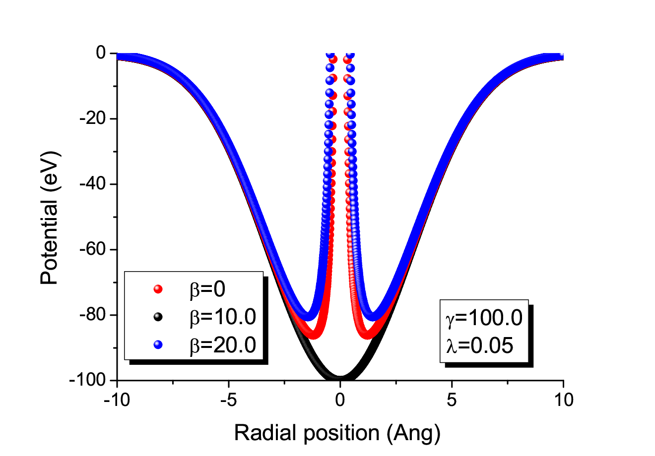
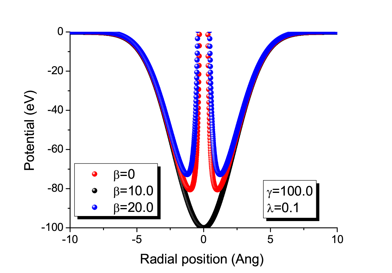
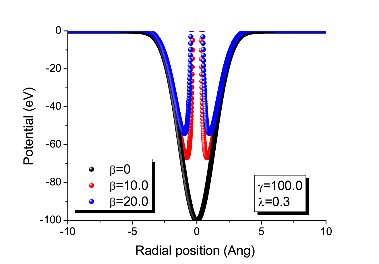
Figure 2 shows the potential introduced in equation (2.7). Due to the additional term (), the electrons in the system will be pushed to make a motion in the regions far from the center of the sphere. The increase in the will cause a decrease of the motion area of the electrons. Therefore, this potential can describe a group of spherical symmetric molecular structures and different types of hollow nanospheres.
3 Theory
As seen from equation (2.7), the potential is constructed with two parts. can be introduced into the barrier term following the previous study by Aygun et al. [32]. In this case, we can describe a new parameter which results in:
| (3.1) |
The attractive Gaussian potential part in equation (2.7) can be expanded as follows
| (3.2) |
where indicates the well known harmonic oscillator potential where . The role of the terms other than is to modify the potential and they may be referred to as modification potentials. The normalized wavefunction of a harmonic oscillator is
| (3.3) |
where and are electron mass and Planck’s constant, respectively, is associated Laguerre polynomial.
Here, the corresponding eigenvalue and superpotential terms of the harmonic oscillator term can be written from the literature [33]
| (3.4) |
Perturbative wavefunctions, energies and superpotentials corresponding to the modification potentials are as follows:
| (3.5) |
where indicates the perturbation order. If the unknown perturbed wavefunction is , the Schrödinger equation can be written as follows:
| (3.6) |
Skipping the details of the calculation procedure of the theory to our previous work [31], the total energy eigenvalues can be written as follows:
| (3.7) |
where . Therefore, we obtain a simple analytical form of the energy eigenvalues.
| 0 | –2.9404 | –1.79436 | –1.20055 | –3.37972 | –2.69002 | –2.32524 | –3.55892 | –3.06275 | –2.79796 |
|---|---|---|---|---|---|---|---|---|---|
| 1 | –1.94631 | –1.30392 | –0.83482 | –2.78255 | –2.3891 | –2.09817 | –3.12967 | –2.84443 | –2.63231 |
| 2 | –1.00933 | –0.5972 | –0.24876 | –2.20674 | –1.94968 | –1.73062 | –2.71159 | –2.52366 | –2.36291 |
| 3 | –0.12217 | 0.4336 | –1.65066 | –1.46551 | –1.2973 | –2.30409 | –2.16762 | –2.0433 | |
| 4 | –1.11281 | –0.9707 | –0.8373 | –1.90659 | –1.80102 | –1.70174 | |||
| 5 | –0.59181 | –0.47792 | –0.36901 | –1.51854 | –1.43333 | –1.35173 | |||
| 6 | –0.08637 | –1.13943 | –1.06854 | –0.99989 | |||||
| 7 | –0.76877 | –0.70845 | –0.6496 | ||||||
| 8 | –0.40612 | –0.35388 | –0.30266 | ||||||
| 9 | –0.05102 | –0.00515 |
| ; | |||||||||
|---|---|---|---|---|---|---|---|---|---|
| 0 | –1.00933 | –2.20674 | –1.56434 | –1.22363 | –2.71159 | –2.24051 | –1.98875 | ||
| 1 | –0.12217 | –1.65066 | –1.28332 | –1.01121 | –2.30409 | –2.03295 | –1.83114 | ||
| 2 | –1.11281 | –0.87216 | –0.66683 | –1.90659 | –1.7277 | –1.57458 | |||
| 3 | –0.59181 | –0.41799 | –0.25992 | –1.51854 | –1.38844 | –1.26988 | |||
| 4 | –0.08637 | –1.13943 | –1.03865 | –0.94383 | |||||
| 5 | –0.76877 | –0.68731 | –0.60927 | ||||||
| 6 | –0.40612 | –0.33824 | –0.27249 |
4 Results and discussion
The change of the parameters in the potential of equation (2.7) refers to the change of the kind of the molecular structure. As can be seen from figure 3, varying the value of parameter it is possible to control the size of the potential well. Furthermore, using the parameter different from zero, it is possible to split the gaussian potential into two parts in the positive and the negative regions. The increase in causes a shrink in the potential.
5 Conclusions
We have obtained an analytical form for the energy eigenvalues of fullerene-type hollow nanospheres by using the technique from our previous study. A simple analytical expression (but not an exact one) is a closed form for the bound states of a modified attractive Gaussian potential by using supersymmetric perturbation theory. The analytical expression can be used to see the treatment of the energy values. Furthermore, we have shown that this potential can be a good candidate to model semiconductor quantum dots and to reveal the electronic and optical properties of the system.
References
- [1] Köksal K., Pavlyukh Ya., Berakdar J., J. Sci. Technol. Bitlis Eren University, 2011, 1, No. 1, 4.
- [2] Martz L., SciBX: Science-Business eXchange, 2013, 6, 11; doi:10.1038/scibx.2013.256.
- [3] Li C., Li L., Keates A.C., Oncotarget, 2012, 3, No. 4, 365.
- [4] Ahn S., Jung S.Y., Lee S.J., In: Proceedings of the Conference ‘‘APS March Meeting’’ (Baltimore, Maryland, 2013), B. Am. Phys. Soc., 2013, 58.
- [5] Salata O.V., J. Nanobiotechnology, 2004, 2, No. 1, 3; doi:10.1186/1477-3155-2-3.
- [6] Akgül S., Şahin M., Köksal K., J. Lumin., 2012, 132, No. 7, 1705; doi:10.1016/j.jlumin.2012.02.012.
- [7] Şahin M., Phys. Rev. B, 2008, 77, 045317; doi:10.1103/PhysRevB.77.045317.
- [8] Harrison P., Quantum Wells, Wires and Dots: Theoretical and Computational Physics of Semiconductor Nanostructures, Wiley, The University of Leeds, 2011.
- [9] Guldi D., Martin N., Fullerenes: From Synthesis to Optoelectronic Properties, Developments in Fullerene Science, Springer, Dordlecht, 2002.
- [10] Ma H., Gao F., Liang W., J. Phys. Chem. C, 2012, 116, No. 2, 1755; doi:10.1021/jp2094092.
- [11] Podsiadlo P., Kwon S.G., Koo B., Lee B., Prakapenka V.B., Dera P., Zhuravlev K.K., Krylova G., Shevchenko E.V., J. Am. Chem. Soc., 2013, 135, No. 7, 2435; doi:10.1021/ja311926r.
- [12] Pavlyukh Y., Berakdar J., Chem. Phys. Lett., 2009, 468, No. 4, 313; doi:10.1016/j.cplett.2008.12.051.
- [13] Pavlyukh Y., Berakdar J., Phys. Rev. A, 2010, 81, 042515; doi:10.1103/PhysRevA.81.042515.
- [14] Zhao J., Wang L., Li F., Chen Z., J. Phys. Chem. A, 2010, 114, No. 37, 9969; doi:10.1021/jp1018873.
- [15] Scuseria G.E., Science, 1996, 271, No. 5251, 942; doi:10.1126/science.271.5251.942.
- [16] Gonzalez Szwacki N., Sadrzadeh A., Yakobson B.I., Phys. Rev. Lett., 2007, 98, No. 16, 166804; doi:10.1103/PhysRevLett.98.166804.
- [17] Halac E., Burgos E., Bonadeo H., Chem. Phys. Lett., 1999, 299, No. 1, 64; doi:10.1016/S0009-2614(98)01226-3.
- [18] Chen Z., Thiel W., Chem. Phys. Lett., 2003, 367, No. 1, 15; doi:10.1016/S0009-2614(02)01660-3.
- [19] Dolmatov V.K., King J.L., Oglesby J.C., J. Phys. B: At. Mol. Opt. Phys., 2012, 45, No. 10, 105102; doi:10.1088/0953-4075/45/10/105102.
- [20] George J., Varma H.R., Deshmukh P.C., Manson S.T., J. Phys. B: At. Mol. Opt. Phys., 2012, 45, No. 18, 185001; doi:10.1088/0953-4075/45/18/185001.
- [21] Grum-Grzhimailo A.N., Gryzlova E.V., Strakhova S.I., J. Phys. B: At. Mol. Opt. Phys., 2011, 44, No. 23, 235005; doi:10.1088/0953-4075/44/23/235005.
- [22] Nascimento E.M., Prudente F.V., Guimares M.N., Maniero A.M., J. Phys. B: At. Mol. Opt. Phys., 2011, 44, No. 1, 015003; doi:10.1088/0953-4075/44/1/015003.
- [23] Lin C.Y., Ho Y.K., J. Phys. B: At. Mol. Opt. Phys., 2012, 45, No. 14, 145001; doi:10.1088/0953-4075/45/14/145001.
- [24] Buck B., Friedrich H., Wheatley C., Nucl. Phys. A, 1977, 275, No. 1, 246; doi:10.1016/0375-9474(77)90287-1.
- [25] Gomez S., Romero R., Cent. Eur. J. Phys., 2009, 7, 12; doi:10.2478/s11534-008-0132-z.
- [26] Adamowski J., Sobkowicz M., Szafran B., Bednarek S., Phys. Rev. B, 2000, 62, 4234; doi:10.1103/PhysRevB.62.4234.
- [27] Coden D.S.A., Gomez S.S., Romero R.H., J. Phys. B: At. Mol. Opt. Phys., 2011, 44, No. 3, 035003; doi:10.1088/0953-4075/44/3/035003.
- [28] Xie W., Superlattices and Microstruct., 2010, 48, No. 2, 239; doi:10.1016/j.spmi.2010.04.015.
- [29] Lu L., Xie W., Hassanabadi H., Physica B, 2011, 406, No. 21, 4129; doi:10.1016/j.physb.2011.07.063.
- [30] Hours J., Senellart P., Peter E., Cavanna A., Bloch J., Phys. Rev. B, 2005, 71, 161306; doi:10.1103/PhysRevB.71.161306.
- [31] Köksal K., Phys. Scripta, 2012, 86, No. 3, 035006; doi:10.1088/0031-8949/86/03/035006.
- [32] Aygun M., Bayrak O., Boztosun I., J. Phys. B: At. Mol. Opt. Phys., 2007, 40, No. 3, 537; doi:10.1088/0953-4075/40/3/009.
- [33] Dabrowska J.W., Khare A., Sukhatme U.P., J. Phys. A: Math. Gen., 1988, 21, No. 4, L195; doi:10.1088/0305-4470/21/4/002.
Простий модельний потенцал для порожнистих наносфер
К. Кьоксал, М. Йонджан?,?, Б. Гьон’юл, Б. Гьон’юл
-
Фзичний факультет, унверситет Ерена м. Бтлс, 13000, Бтлс, Туреччина
-
Факультет нженерно фзики, унверситет м. Газантеп, 27100, Газантеп, Туреччина