An Accurate and Efficient Analysis of a MBSFN Network

Multicast-broadcast single-frequency network (MBSFN) is a transmission mode defined in the Long Term Evolution (LTE) standard [1], and in particular for the Multimedia Broadcast Multicast Service (MBMS) [2]. MBSFN is designed to send multicast or broadcast data as a multicell transmission over a synchronized single-frequency network (SFN). A group of those cells that are targeted to receive the same data is called an MBSFN area. MBSFN enables the efficient delivery of applications such as mobile TV, radio broadcasting, file delivery and emergency alerts without the need of additional expensive licensed spectrum and without requiring new infrastructure and end-user devices. The transmissions from the different base stations in an MBSFN area are tightly synchronized and the MBSFN transmission appear to a user equipment (UE) as a transmission from a single large cell, with each base station transmission appearing as a separate multipath component, dramatically increasing the signal-to-interference-noise ratio (SINR). Since only transmissions from base stations that lie outside the MBSFN area are interference, the intercell interference is reduced [3].

This paper presents a new and precise analysis for MBSFN orthogonal frequency-division multiple access (OFDMA) networks. The analysis is driven by a new closed-form expression for the outage probability conditioned with respect to the network topology and shadowing. In particular, in [4] a closed-form expression is derived for conventional networks, and in [5] it has been extended when signals arriving over different paths can be resolved in the presence of noise and interference. The channel model accounts for path loss, correlated shadowing, and Nakagami fading, and the Nakagami fading parameters do not need to be identical for all links.

In contrast with other works on MBSFN networks [3, 6, 7, 8], we don’t use the classical approach to model cellular networks; i.e., we do not assume that the base stations are placed according to a lattice or regular grid. Rather, we assume that the base-station locations are modeled as a realization of a random point process [9, 10, 11, 12, 13]. In particular, in order to model the network more realistically, a uniform cluster model is used, which the authors have recently adopted to analyze both the downlink [14] and the uplink [15] of a conventional non-cooperative cellular network. Having adopted a realistic model and an accurate analysis, the influence of the minimum base-station separation is investigated and insight provided regarding the optimal size of the MBSFN areas. Furthermore, in this paper we propose to quantify performance using the area below an outage threshold (ABOT), which is here defined to be the fraction of the network that meets an outage constraint. The ABOT gives a useful indication of the percentage of the network that will successfully receive the broadcast.

The network comprises $M$ cellular base stations $\{X_{1},...,X_{M}\}$ placed on a finite square area $A_{\mathsf{net}}$ with sides of length $d_{\mathsf{net}}$. The variable $X_{i}$ represents both the $i^{th}$ base station and its location. To facilitate the analysis, the coverage area of the network is discretized into a large number of points, and the variable $Y_{j}$ is used to indicate the location of the $j^{th}$ point within the network. Each location $Y_{j}$ within a radio cell receives the same content from one or multiple base stations, which belongs to an MBSFN area. In each MBSFN area, the same content is synchronously broadcasted. Let $\mathcal{G}_{j,z}$ denote the set of the indexes of the base stations that belong to the $z^{th}$ MBSFN area and serving location $Y_{j}$. Furthermore, let $\mathcal{Z}_{j}$ denote the index of the MBSFN area that covers the location $Y_{j}$ and $N_{j}=|\mathcal{G}_{j,\mathcal{Z}_{j}}|$ be the number of base stations that belongs to that area.

The base stations are deployed according to a uniform-clustering model [4]. Using this model, the $M$ base stations are uniformly deployed in the network area $A_{\mathsf{net}}$. An exclusion zone of radius $r_{bs}$ surrounds each base station, and no other base stations are allowed within this zone. In particular, each base station is placed one at a time uniformly into the portion of the network that remains outside of the exclusion zones of the previously placed base stations. The radius of the base-station exclusion zones can be primarily determined by economic considerations and the terrain.

The network comprises $S$ MFSFN areas, which are defined as follows. Inside the network arena, $\{Z_{1},...,Z_{S}\}$ points are picked according to a regular hexagonal grid and equally separated by $d_{\mathsf{sfn}}$, where the variable $Z_{z}$ represents the $z^{th}$ location. The $z^{th}$ MBSFN area is then formed by the radio cells of all base stations that are closer to the location of $Z_{z}$.

In a MBSFN OFDMA network, the transmissions are tightly synchronized and it is possible to combine the signals that are sent by all base stations $X_{i},i\in\mathcal{G}_{j,\mathcal{Z}_{j}}$ and received at the UE, located at position $Y_{j}$, if the signals arrive within the extended cyclic prefix, which is fixed to be equal to $T_{ECP}=16.7\mu s$ [16]. The signal from base station $X_{i},i\in\mathcal{G}_{\mathcal{Z}_{j}}$ to the UE at location $Y_{j}$ is then included in the MRC combined signal passed to the demodulator, if $||X_{i}-Y_{j}||<d_{\mathsf{max}}$, where $d_{\mathsf{max}}=5$ km, otherwise it results in inter-symbol interference (ISI). The set $\mathcal{G}_{j,z}$ contains the indices of those base stations that are closer to $Z_{\mathcal{Z}_{j}}$ and they are located such that their signals arrive at $Y_{j}$ within the extended cyclic prefix. The set $\mathcal{G}_{j,z}$ is then selected such that $i\in\mathcal{G}_{j,\mathcal{Z}_{j}}$ if $||Z_{\mathcal{Z}_{j}}-X_{i}||<||Z_{s}-X_{i}||$, $\forall s\neq\mathcal{Z}_{j}$ and also if $||X_{i}-Y_{j}||<d_{\mathsf{max}}$.

Let $\rho_{i,j}$ represent the instantaneous received power of $X_{i}$ at location $Y_{j}$, which depends on the path loss, shadowing, and fading. We assume that the path loss has a power-law dependence on distance. In particular, for a distance $d\geq d_{0}$, the path-loss function is expressed as the attenuation power law

where $\alpha\geq 2$ is the attenuation power-law exponent, and it is assumed that $d_{0}$ is sufficiently large that the signals are in the far field.

Let $d_{i,j}=||X_{i}-Y_{j}||$ be the distance between base station $X_{i}$ and location $Y_{j}$. The instantaneous power of the signal received at the location $Y_{j}$ from the base station $X_{i}$ is

where $P_{0}$ is the transmit power, which is common for all base stations, $g_{i,j}$ is the power gain due to fading and $\xi_{i,j}$ is a shadowing factor. The $\{g_{i,j}\}$ are independent with unit-mean, and $g_{i,j}=a_{i,j}^{2}$, where $a_{i,j}$ is Nakagami with parameter $m_{i,j}$. While the $\{g_{i,j}\}$ are independent from mobile to mobile, they are not necessarily identically distributed, and for each mobile each link between $Y_{j}$ and $X_{i}$ can be characterized by a distinct Nakagami parameter $m_{i,j}$. When the channel between $X_{i}$ and $Y_{j}$ experiences Rayleigh fading, $m_{i,j}=1$ and $g_{i,j}$ is exponentially distributed. It is assumed that the {$g_{i,j}\}$ remain fixed for the duration of a MBSFN subframe, but vary independently from subframe to subframe. In the presence of log-normal shadowing, the $\{\xi_{i,j}\}$ are zero-mean Gaussian with variance $\sigma_{s}^{2}$ and characterized by the normalized autocorrelation function $\mathcal{R}\left(\Delta x\right)$, where $\Delta x$ is the change in distance. The normalized autocorrelation function can be described with sufficient accuracy by an exponential function as [17]

with the decorrelation length $d_{\mathsf{corr}}$ , which is dependent on the environment. For the urban vehicular test environment (VTE), [18] proposes $d_{\mathsf{corr}}=20$ m. This correlation works satisfactorily for distances up to approximately $500$ m. In the absence of shadowing, $\xi_{i,j}=0$.

A distance-dependent fading model is assumed, where a signal originating at base station $X_{i}$ arrives at location $Y_{j}$ with a Nakagami fading parameter $m_{i,j}$ determined as following

where $r_{\mathsf{f}}$ is the line-of-sight radius. The distance-dependent-fading model characterizes the situation where a mobile close to the base station is in the line-of-sight, while mobiles farther away are usually not.

The instantaneous SINR at location $Y_{j}$ by using (1) and (2) can be expressed as [6]

where $\Gamma=d_{0}^{\alpha}N_{j}P_{0}/\mathcal{N}$ is the signal-to-noise ratio (SNR) at a mobile located at unit distance when fading and shadowing are absent, $\mathcal{N}$ is the noise power, and

is the normalized power of $X_{i}$ at receiver $Y_{j}$.

Let $\beta$ denote the minimum SINR required at location $Y_{j}$ for reliable reception and $\boldsymbol{\Omega}_{j}=\{\Omega_{1,j},...,\Omega_{M,j}\}$ represent the set of normalized base-station powers received at $Y_{j}$. An outage occurs when the SINR falls below $\beta$. As discussed subsequently, there is a relationship between the SINR threshold and the supported rate of the transmission. Conditioning on $\boldsymbol{\Omega}_{j}$, the outage probability of mobile $Y_{j}$ is

Because it is conditioned on $\boldsymbol{\Omega}_{j}$, the outage probability depends on the particular network realization, which has dynamics over timescales that are much slower than the fading. By defining

the conditional outage probability may be expressed as

which is the cumulative distribution function (cdf) of $\mathsf{Z}_{j}$ conditioned on $\boldsymbol{\Omega}_{j}$ and evaluated at $\Gamma^{-1}$. Restricting the Nakagami parameter $m_{i,j}$ between location $Y_{j}$ and base station $X_{i}$ to be integer-valued, the cdf of $\mathsf{Z}_{j}$ conditioned on $\boldsymbol{\Omega}_{j}$ is proved in [5] to be (11) at the top of this page. The function $\Xi_{L}\left(k,n,\left\{r_{q}\right\}_{q=1}^{L},\left\{\eta_{q}\right\}_{q=1}^{L}\right)$ is defined by (12) at the top of this page, where $u(x)$ is the step function and $R_{L}=\sum_{k=1}^{L}r_{k}.$

In order to analyze the network performance, the area below an outage threshold (ABOT) is used, which is defined as the fraction of the network realization $t$ that provides an outage probability (averaged over the fading) that meets a threshold

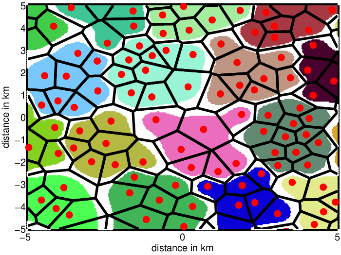
The ABOT is an indicator of the percentage of the network that will successfully receive the broadcast. An outage threshold of $\hat{\epsilon}=0.1$ is typical and appropriate for modern systems. For instance, in Fig.1 it is shown a portion of an example network, where the area in white is the portion of the network for which the outage probability is above $\hat{\epsilon}=0.1$ with $\beta=0$ dB, $\Gamma=10$ dB and $\alpha=3.5$, which as expected corresponds to the edge of the MBSFN areas, that are here illustrated with different colors and obtained by fixing $d_{\mathsf{sfn}}=3$. The base-station exclusion radius is fixed to $r_{bs}=0.5$, $M=400$ base stations are deployed into a square network arena with side of length $d_{\mathsf{net}}=20$. The base station locations are given by the large filled circles and the Voronoi tessellation shows the radio cell boundaries that occur in the absence of shadowing.

After computing $\mathcal{A}_{\mathsf{bot}}^{\left(t\right)}$ for $\Upsilon$ network topologies, its spatial average can be computed as following

A key consideration in the operation of the network is the manner that base stations select their rates at which the multimedia content is broadcasted. The SINR threshold depends on the modulation and coding scheme and receiver implementation. For a given $\beta$, there is a corresponding transmission rate $R$ that can be supported, and typically only a discrete set of $R$ can be supported. Let $R=C(\beta)$ represent the relationship between $R$, expressed in units of bits per channel use (bpcu), and $\beta$. While the exact dependence of $R$ on $\beta$ can be determined empirically through tests or simulation, we make the simplifying assumption when computing our numerical results that $C(\beta)=\log_{2}(1+\beta)$ corresponding to the Shannon capacity for complex discrete-time AWGN channels. This assumption is fairly accurate for systems that use capacity-approaching codes and a large number of code rates and modulation schemes, such as modern cellular systems, which use turbo codes with a large number of available modulation and coding schemes.

In order to determine the rate $R$ for a typical network the following approach is used. Draw a realization of the network by placing base stations according to a uniform clustering model with density $\lambda=M/A_{net}$. Group the base stations into MBSFN areas. Compute the path loss from each base station to a very large number of locations, selected such that they form an extremely dense grid that covers the entire network arena, applying randomly generated correlated shadowing factors if shadowing is present. Determine the outage probabilities by using (11) parameterized by the SINR threshold for all locations. By applying the function $R=C(\beta)$, find the corresponding rate.

As an example, consider a square network area with sides of length $d_{\mathsf{net}}=20$, where the performance is evaluated only in the center $10\times 10$ portion of the network, in order to exclude edge effects. The base-station exclusion zone is set to $r_{\mathsf{bs}}=0.5$ and the outage constraint is set to $\hat{\epsilon}=0.1$. The line-of-sight radius is $r_{\mathsf{f}}=0.5$. Other fixed parameter values are $\alpha=3.5$, $\Gamma=10$ dB and $\Upsilon=1000$.

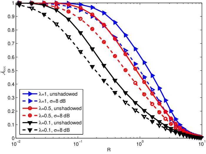
Fig. 3 shows the ABOT as function of the rate for both a shadowed ($\sigma_{s}=8$ dB) and an unshadowed scenario and for three values of lambda when $d_{\mathsf{sfn}}=6$: (1) $\lambda=1$, (2) $\lambda=0.5$ and (3) $\lambda=0.1$. Fig. 3 shows that there is a tradeoff between the two quantities. Shadowing is detrimental and an increase in the density of base-station results in an higher ABOT. Fig. 3 shows the ABOT as function of the outage threshold parameterized for three values of $d_{\mathsf{sfn}}$ when $\lambda=0.5$ and $R=0.5$. Fig. 3 shows that an increase in the size of the MBSFN areas results in an improvement in performance, but only until a certain value. After a certain value of $d_{\mathsf{sfn}}$, the ISI starts to increase and the regions at the edge of the MBSFN areas don’t get any more benefit by increasing them furthermore. Fig. 4 shows the area below an outage threshold as function of the minimum separation among base-station when $R=0.1$,$\lambda=0.1$ and $d_{\mathsf{sfn}}=6$. The curves are shown for both a shadowed ($\sigma_{s}=8$ dB) and an unshadowed scenario and for both Rayleigh fading ($r_{f}=0$) and a distance-depending fading when $r_{bs}=r_{f}$. Fig. 4 shows that the fraction of network that succeeds to meet an outage constraint increases when the base-stations have an higher minimum separation and this effect is more prominent under a distance-depending fading.

This paper has presented a new approach for modeling and analyzing the performance of multicast-broadcast single-frequency network (MBSFN). The analysis combines a new outage probability expression, which is exact for a given network realization, with a constrained random spatial model, which allows the statistics to be determined for a class of network topologies. The results show that an increase in the size of an MBSFN areas leads to an improvement in performance only until a certain value of $d_{\mathsf{sfn}}$ is reached and as expected performance increases as the minimum separation among base-station gets higher.

References

- [1] European Telecommunications Standards Institute, “LTE; Evolved universal terrestrial radio access network (E-UTRAN); X2 application protocol (X2AP),” 3GPP TS 136.423 version 11.4.0, Mar. 2013.
- [2] European Telecommunications Standards Institute, “Universal mobile telecommunications system (UMTS); LTE; multimedia broadcast/multicast service (MBMS); protocols and codecs,” 3GPP TS 126.346 version 11.4.0, Apr. 2013.
- [3] A. Alexiou, C. Bouras, V. Kokkinos, A. Papazois, and G. Tsichritzis, “Spectral efficiency performance of MBSFN-enabled LTE networks,” in Proc. IEEE Int. Conf. on Wireless & Mobile Comp., Network. and Commun., Niagara Falls, Canada, Oct. 2010.
- [4] D. Torrieri and M. C. Valenti, “The outage probability of a finite ad hoc network in Nakagami fading,” IEEE Trans. Commun., vol. 60, pp. 3509–3518, Nov. 2012.
- [5] S. Talarico, M. C. Valenti, and D. Torrieri, “Analysis of multi-cell downlink cooperation with a constrained spatial model,” in Proc. IEEE Global Telecommun. Conf. (GLOBECOM), Atlanta, GA, Dec. 2013.
- [6] L. Rong, O. Haddada, and S. Elayoubi, “Analytical analysis of the coverage of a MBSFN OFDMA network,” in Proc. IEEE Global Telecommun. Conf. (GLOBECOM), New Orleans, LA, Dec. 2008.
- [7] A. Alexiou, C. Bouras, V. Kokkinos, and G. Tsichritzis, “Communication cost analysis of MBSFN in LTE,” in Proc. IEEE Personal Indoor and Mobile Radio Commun. Conf., Istanbul, Turkey, Sept. 2010.
- [8] A. Alexiou, C. Bouras, V. Kokkinos, and G. Tsichritzis, “Performance evaluation of LTE for MBSFN transmissions,” Wireless Networks, vol. 18, pp. 227–240, Apr. 2012.
- [9] R. K. Ganti and M. Haenggi, Interference in Large Wireless Networks, vol. 3, Now, Paris, 2009.
- [10] F. Baccelli and B. Błaszczyszyn, Stochastic Geometry and Wireless Networks - Volume I: Theory, vol. 3, Now, Paris, 2009.
- [11] F. Baccelli and B. Błaszczyszyn, Stochastic Geometry and Wireless Networks - Volume II: Applications, vol. 4, Now, Paris, 2009.
- [12] J. Andrews, F. Baccelli, and R. K. Ganti, “A tractable approach to coverage and rate in cellular networks,” IEEE Trans. Commun., vol. 59, pp. 3122–3134, Nov. 2011.
- [13] M. Haenggi, Stochastic Geometry for Wireless Networks, Cambridge University Press, Paris, 2012.
- [14] M. C. Valenti, D. Torrieri, and S. Talarico, “A new analysis of the DS-CDMA cellular downlink under spatial constraints,” in Proc. IEEE Int. Conf. on Comp., Network. and Commun., San Diego, CA, Jan. 2013.
- [15] D. Torrieri, M. C. Valenti, and S. Talarico, “An analysis of the DS-CDMA cellular uplink for arbitrary and constrained topologies,” IEEE Trans. Commun., vol. 61, pp. 3318–3326, Aug. 2013.
- [16] E. Dahlman, S. Parkvall, and J. Skold, 4G LTE/LTE-Advanced for Mobile Broadband, Academic Press, 2011.
- [17] M. Gudmundson, “Correlation model for shadow fading in mobile radio systems,” Electronics Letters, vol. 27, pp. 2145 – 2146, Nov. 1991.
- [18] European Telecommunications Standards Institute, “Universal mobile telecommunications system (UMTS);selection procedures for the choice of radio transmission technologies of the UMTS (UMTS 30.03),” TR 101 112, Apr. 1998.