Order Reduction of the Chemical Master Equation via Balanced Realisation

Fernando López-Caamal Affiliation: Integrative Systems Biology Unit, Okinawa Institute of Science and Technology, Kunigami, Okinawa 904-0412, Japan Tatiana T. Marquez-Lago^* Affiliation: ^* Author for correspondence: tatiana.marquez@oist.jp

August 24, 2026

Abstract

We consider a Markov process in continuous time with a finite number of discrete states. The time-dependent probabilities of being in any state of the Markov chain are governed by a set of ordinary differential equations, whose dimension might be large even for trivial systems. Here, we derive a reduced ODE set that accurately approximates the probabilities of subspaces of interest with a known error bound. Our methodology is based on model reduction by balanced truncation and can be considerably more computationally efficient than the Finite State Projection Algorithm (FSP) when used for obtaining transient responses. We show the applicability of our method by analysing stochastic chemical reactions. First, we obtain a reduced order model for the infinitesimal generator of a Markov chain that models a reversible, monomolecular reaction. In such an example, we obtain an approximation of the output of a model with $301$ states by a reduced model with $10$ states. Later, we obtain a reduced order model for a catalytic conversion of substrate to a product; and compare its dynamics with a stochastic Michaelis-Menten representation. For this example, we highlight the savings on the computational load obtained by means of the reduced-order model. Finally, we revisit the substrate catalytic conversion by obtaining a lower-order model that approximates the probability of having predefined ranges of product molecules.

I Introduction

Markov chains are versatile dynamical systems that model a broad spectrum of physical, biological, and engineering systems. Along with the broad range of its applications, one of the main advantages of Markov chains is that some of them can be easily handled and cast as time-invariant, linear systems [1, 2, 3].

In this paper, we focus on continuous-time, discrete-state, homogeneous, irreducible Markov chains with a finite number of states. The probability of being in any state is governed by a linear set of ordinary differential equations (ODEs), where individual ODEs correspond to each state of the system, describing all possible transitions in and out of such states. This set of ODEs is commonly referred to as forward Kolmogorov equation or Chemical Master equation and might have large dimensions even for simple systems. Hence, obtaining a solution for such a system might be analytically intractable and computationally demanding.

Provided that one is interested only in some states or a combination of states of the Markov chain, it is possible to obtain a reduced order model via the balanced realisation of the linear system that describes the probability of being in such states. The reduced model has a smaller number of coupled differential equations, yet approximates the output of the full model with an error bound proportional to the sum of the Hankel Singular Values neglected to obtain the reduced model [4, 5, 6, 7]. Since chemical reaction networks in a homogeneous media with a low number of molecules, and in thermodynamic equilibrium can be described as Markov chains, it is possible to apply our methodology to this class of systems.

There exist alternative approaches to obtain reduced order models from the CME. For instance, the Finite State Projection Method obtains the probability density function in prescribed subsets of the state space and for a specific time point [8]. From this method, it is also possible to obtain a linear set of ODEs that can, in general, be further reduced via the methodology we use in this paper. Other approaches make use of Krylov subspaces to approximate the solution of the exponential matrix that generates the solutions of the Markov chain [9, 10]. Additionally, when the species can be classified by its behaviour into stochastic or deterministic, [11] propose a methodology in which the CME can be solved directly and efficiently, when the number of species with stochastic behaviour is low. In this direction, works like [12] avail of a time scale separation to estimate the solution of the fast-varying species; and use this estimation to approximate the trajectories of the slow-varying species. On a different perspective, [13] analysed methods to approximate the solution of selected states of the CME, when such solutions can be expressed as the product of two probability density functions: one that describes probabilities of states of interest and a second that depends on the rest of states. This later probability distribution can be approximated by its mean, for instance, so as to yield an approximated probability density function for those probabilities of interest. However, this approach might yield coarse results if the underlying assumptions are crude.

As an alternative, when the analytical or computational treatment of the Markov chain is infeasible, it is common to opt for numerical simulations of the stochastic system and analyse the outcome statistically. [14], and [15], among many others, provide surveys of simulation methods of stochastic reaction networks. However, these methods might require large computational times to yield accurate results.

A different way to reduce the CMEs is to consider subsystems that focus on features of interest. In the chemical context, [16] showed as a proof-of-concept that the simple reaction $S_{1}{}\mathrel{\hbox to0.0pt{\raisebox{0.94722pt}{$\mathrel{\mathop{\makebox[0.0pt]{\to}}\limits^{\mkern 9.0muk_{1}\mkern 9.0mu}_{\makebox{\raisebox{3.76735pt}[0.0pt]{$\scriptstyle\mkern 9.0mu\hphantom{k_{2}}\mkern 5.0mu$}}}}$}\hss}\raisebox{-0.94722pt}{$\mathrel{\mathop{\makebox[0.0pt]{\to}}\limits^{\mkern 5.0mu\hphantom{k_{1}}\mkern 9.0mu}_{\makebox{\raisebox{3.76735pt}[0.0pt]{$\scriptstyle\mkern 9.0muk_{2}\mkern 9.0mu$}}}}$}}{}S_{2}{}\mathrel{\mathop{\makebox[0.0pt]{\rightarrow\displaystyle}}\limits^{\mkern 5.0muk_{3}\mkern 9.0mu}}{}S_{3}$ can only be accurately represented by $S_{1}{}\mathrel{\mathop{\makebox[0.0pt]{\rightarrow\displaystyle}}\limits^{\mkern 5.0muk\mkern 9.0mu}}{}S_{3}$ under special conditions on the parameters $k_{1},k_{2},k_{3}$ , which render the dynamics of the species $S_{2}$ irrelevant for the behaviour of $S_{3}$ . This study highlights the shortcomings of neglecting species within a stochastic reaction network. In this paper, we adopt a different approach and overcome these difficulties by deriving a reduced-order model. Such reduced-order model accurately approximates the dynamics of the underlying Markov chain for selected states of any chain with any kind of reaction propensities.

There exist, however, exact approaches that abridge specific topologies of reaction networks. For instance, in [17, 18] different classes of monomolecular reaction networks are exactly represented as reactions characterised by delay distributions. In turn, works like [19, 20] are committed to obtain exact analytical solutions of stochastic chemical reaction networks with linear and nonlinear reactions. Importantly, once a reduced ODE set via balanced realisation is obtained, one can avail of the results in [19] to derive a closed-form expression for approximation of the CME solution.

We illustrate our methodology with the analysis of a reversible, stochastic reaction whose CME has $301$ states. In contrast, an adequate reduced order model has only $10$ states and yield an $\mathcal{L}_{2}$ gain of the approximation error of $587.9172\times 10^{-6}$ . Later, we obtain a reduced order model that approximates the catalysed conversion of a substrate to a product, even in cases in which a stochastic Michaelis-Menten approximation fails to obtain accurate results [21]. For such a system, the simulation of the reduced model may be several orders of magnitude faster than the simulation of the CME. However, there exist an initial cost in computational time to derive the reduced order model. Hence, obtaining the model reduction is profitable when the lower-dimensional ODE set is used repeatedly. Finally, we derive a model that approximates the probability of having predefined ranges of product molecules, in the same catalytic substrate conversion.

II Mathematial Background

II-A Continuous-Time, Discrete-State, Homogeneous Markov Chain

Consider a discrete and finite set of states

\displaystyle\mathbf{S}=\left\{\mathbf{s}^{i}\in\mathbb{Z}^{n},\>\forall\,i\in[1,w]\right\}

(1)

and let the system’s state at time $\mathnormal{t}$ be denoted by $\mathbf{s}(\mathnormal{t}):\mathbb{R}_{+}\to\mathbf{S}$ . Moreover, we consider that the transition from one state to another can be modelled by a time-homogeneous Markov chain, i.e., the next state, $\mathbf{s}(\mathnormal{t}+\mathrm{d}\mathnormal{t})$ , only depends on the current state, $\mathbf{s}$ ( $\mathnormal{t}$ ), independently of $\mathnormal{t}$ . We use $p_{i}(\mathnormal{t}):\mathbb{R}_{+}\times\mathbf{S}\to[0,1]\subset\mathbb{R}$ to denote the probability, $\mathrm{Pr\left(\circ\right)}$ , of the system’s state to be $\mathbf{s}^{i}$ at time $\mathnormal{t}$ . This notation and the Markov property add up to

p_{i}(\mathnormal{t}+\mathrm{d}\mathnormal{t})=\mathrm{Pr}\left(\mathbf{s}(\mathnormal{t}+\mathrm{d}\mathnormal{t})=\mathbf{s}^{i}|\mathbf{s}(\mathnormal{t})\right).

We gather the probabilities for every state in the column vector

\mathbf{p}(\mathnormal{t}):=(p_{1}(\mathnormal{t})\quad\ldots\quad p_{w}(\mathnormal{t}))^{T}.

(2)

Let us denote the transition probability from state $j$ to state $i$ at time $\mathnormal{t}+\tau$ by $q_{ij}(\mathnormal{t}+\tau):\mathbb{R}_{+}\times\mathbf{S}^{2}\to[0,1]$ . That is to say,

q_{ij}(\mathnormal{t}+\tau):=\mathrm{Pr\left(\mathbf{s}(\mathnormal{t}+\tau)=\mathbf{s}^{i}|\mathbf{s}(\mathnormal{t})=\mathbf{s}^{j}\right)}.

The time-homogeneity property of the Markov chain implies

$\displaystyle q_{ij}(\mathnormal{t}+\tau)$	$\displaystyle:=$
$\displaystyle\mathrm{Pr\left(\mathbf{s}(\mathnormal{t}+\tau)=\mathbf{s}^{i}\|\mathbf{s}(\mathnormal{t})=\mathbf{s}^{j}\right)}$	$\displaystyle=$
$\displaystyle\sum_{k=1}^{w}\mathrm{Pr\left(\mathbf{s}(\mathnormal{t}+\tau)=\mathbf{s}^{i};\mathbf{s}(\tau)=\mathbf{s}^{k}\|\mathbf{s}(0)=\mathbf{s}^{j}\right)}$	$\displaystyle=$
$\displaystyle\sum_{k=1}^{w}\mathrm{Pr\left(\mathbf{s}(\mathnormal{t}+\tau)=\mathbf{s}^{i}\|\mathbf{s}(\tau)=\mathbf{s}^{k};\mathbf{s}(0)=\mathbf{s}^{j}\right)}$
$\displaystyle\times\mathrm{Pr\left(\mathbf{s}(\tau)=\mathbf{s}^{k}\|\mathbf{s}(0)=\mathbf{s}^{j}\right)}$	$\displaystyle=$
$\displaystyle\sum_{k=1}^{w}q_{ik}(\mathnormal{t})q_{kj}(\tau)$	.	(3)

In matrix form (3), known as Chapman-Kolmogorov equation, is

\displaystyle\mathbb{R}_{+}\to[0,1]^{w\times w}:\mathbf{Q}(\mathnormal{t}+\tau)=\mathbf{Q}(\mathnormal{t})\mathbf{Q}(\tau)=\mathbf{Q}(\tau)\mathbf{Q}(\mathnormal{t}).

(4)

This matrix gathers all the transition probabilities as a function of time and, by consequence, its columns add to one for all $\mathnormal{t}$ . Additionally, if the Markov chain is irreducible, $\mathbf{Q}$ has a simple eigenvalue $\lambda_{1}=1$ , and $\lambda_{1}>\left|\lambda_{i}\right|\,\forall\,1<i\leq w$ . This is consequence of the Perron-Frobenius Theorem as described in [2, Ch. 6], for example. In the rest of this paper, we will deal with finite, irreducible, homogeneous, continuous-time, discrete-state Markov chains exclusively.

Our main interest is to determine the time-dependent probabilities of being in any state of the chain. To this end, we consider the infinitesimal generator of the Markov chain defined as

\displaystyle\mathcal{A}:=

\displaystyle\lim_{\tau\to 0}\frac{\mathbf{Q}(\tau)-\mathbf{I}}{\tau}.

(5)

The elements of the matrix above are

\displaystyle a_{ij}

\displaystyle=\lim_{\tau\to 0}\frac{q_{ij}(\tau)-\delta_{ij}}{\tau},

(6)

where it can be shown that the elements $a_{ij}$ satisfy

\displaystyle a_{ii}=-\sum_{j=1,j\neq i}^{w}a_{ij}.

The last relationship above shows that every column of $\mathcal{A}$ adds up to zero, provided each column of $\mathbf{Q}(\circ)$ add up to one.

It is well-known that $\mathcal{A}$ is the generator of the positive semigroup that governs the evolution of $\mathbf{p}$ ( $\mathnormal{t}$ ) (see [22, Sec. 5.6], for instance):

\displaystyle\frac{\mathrm{d}}{\mathrm{d}\mathnormal{t}}\mathbf{p}(\mathnormal{t})=\mathcal{A}\mathbf{p}(\mathnormal{t}),\quad\mathbf{p}(0)=\mathbf{p}_{0}.

(7)

Under our assumptions, the Markov chain is irreducible and with a finite number of states. Hence, $\mathbf{Q}$ has a unique Frobenius eigenvalue with algebraic multiplicity one [23]. The simple Perron-Frobenius eigenvalue of the stochastic matrix $\mathbf{Q}$ in (4) is 1. Now, let $\boldsymbol{\nu}$ and $\lambda$ be the right Perron-Frobenius eigenvector and eigenvalues of $\mathbf{Q}$ , then the eigenvalues of $\mathcal{A}$ satisfy

	$\displaystyle\mathcal{A}\boldsymbol{\nu}$	$\displaystyle=(\mathbf{Q}-\mathbf{I})\boldsymbol{\nu}/\tau,$
		$\displaystyle=(\lambda-1)\boldsymbol{\nu}/\tau.$

That is, $\mathcal{A}$ preserves the configuration of the eigenvalues of $\mathbf{Q}$ , upon shifting one unit to the left and rescaling. This implies that $\mathcal{A}$ has a zero eigenvalue and the rest of its eigenvalues have negative real part, as confirmed by analysing the Gershgorin circles of the columns of $\mathcal{A}$ .

Note that the dimension of $\mathbf{p}(\circ)$ , $w$ , might be large as it represents all the configurations of a system with $n$ characteristics. In the population and biochemical context, $n$ represents the number of species, whereas $w$ is the number of all the possible combination of species’ population counts. In the following section, we model a stochastic chemical reaction network with the Markov chains described above.

II-B Chemical Master Equation

Now, let us consider $n$ species in a homogeneous medium and in thermodynamic equilibrium and a set of $m$ reactions represented by

\sum_{i=1}^{n}\alpha_{ij}S_{i}{}\mathrel{\mathop{\makebox[0.0pt]{\rightarrow\displaystyle}}\limits^{\mkern 5.0mua_{j}\mkern 9.0mu}}{}\sum_{i=1}^{n}\beta_{ij}S_{i}.

(8)

Let the entries of the stoichiometric matrix $\mathbf{N}\in\mathbb{N}^{n\times m}$ be

\displaystyle n_{ij}:=\beta_{ij}-\alpha_{ij}.

Furthermore, let us consider a vector comprised of the number of molecules, $s_{i}(\mathnormal{t})$ , for every species, $S_{i}$ :

\mathbf{s}(\mathnormal{t})=\left(s_{1}(\mathnormal{t})\quad s_{2}(\mathnormal{t})\quad\ldots\quad s_{n}(\mathnormal{t})\right)^{T}:\mathbb{R}_{+}\to\mathbf{S}.

(9)

The finite set $\mathbf{S}$ above was defined in (1) and contains, at least, all the possible combinations of the species’ molecular numbers in the reaction network. Consider that the $i$ ^th reaction is the only reaction happening within the interval $(\mathnormal{t},\mathnormal{t}+\tau]$ . Hence the number of molecules at time $t+\tau$ is

\mathbf{s}(\mathnormal{t}+\tau)=\mathbf{s}(\mathnormal{t})+\mathbf{n}^{i},

(10)

where $\mathbf{n}^{i}$ represents the $i$ ^th column of $\mathbf{N}$ .

This reaction network may be modelled by the continuous-time, discrete-state jump Markov process described in Section II-A. The states of the Markov chain are the elements in $\mathbf{S}$ . In turn, the vector $\mathbf{p}(\mathnormal{t})$ in (2) gathers the time-dependent probabilities of being in every state, whose time evolution is governed by (7). Additionally, the stochastic behaviour of thermally stable and spatially homogeneous reaction networks has been described[24], where the transition rates between states of the system are shown in Table I.

TABLE I: Reactions and their propensity function. The symbol

s_{i}

denotes the number of molecules of the species

S_{i}

. The symbol

a_{i}

denotes the propensity of reaction

i

Reaction	Propensity
$0{}\mathrel{\mathop{\makebox[0.0pt]{\rightarrow\displaystyle}}\limits^{\mkern 5.0muk_{1}\mkern 9.0mu}}{}S_{1}$	$a_{1}=k_{1}$
$S_{2}{}\mathrel{\mathop{\makebox[0.0pt]{\rightarrow\displaystyle}}\limits^{\mkern 5.0muk_{2}\mkern 9.0mu}}{}X$	$a_{2}(s_{2}(\mathnormal{t}))=k_{2}s_{2}(\mathnormal{t})$
$S_{3}+S_{4}{}\mathrel{\mathop{\makebox[0.0pt]{\rightarrow\displaystyle}}\limits^{\mkern 5.0muk_{3}\mkern 9.0mu}}{}X$	$a_{3}(s_{3}(\mathnormal{t}),s_{4}(\mathnormal{t}))=k_{3}s_{3}(\mathnormal{t})s_{4}(\mathnormal{t})$
$2S_{5}{}\mathrel{\mathop{\makebox[0.0pt]{\rightarrow\displaystyle}}\limits^{\mkern 5.0muk_{4}\mkern 9.0mu}}{}X$	$a_{4}(s_{5}(\mathnormal{t}))=k_{4}s_{5}(\mathnormal{t})(s_{5}(\mathnormal{t})-1)/\penalty 2\quad s_{5}(\mathnormal{t})\geq 1$

To construct the matrix $\mathcal{A}$ in (7), we have to evaluate the probabilities’ transition rate for all states $\mathbf{s}^{i}\in\mathbf{S}$ and arrange them as the entries of $\mathcal{A}$ as follows

\mathcal{A}_{ji}=\begin{cases}-\sum_{k=1}^{m}a_{k}(\mathbf{s}^{i}),&i=j,\\ a_{k}(\mathbf{s}^{i}),&\forall\,j:\mathbf{s}^{j}=\mathbf{s}^{i}+\mathbf{n}^{k},\\ 0,&\textnormal{otherwise}.\end{cases}

(11)

In the next section, we present a methodology used to obtain reduced order models, which are capable of reproducing the dynamical behaviour of a linear system with a smaller number of ODEs.

II-C Balanced Model Reduction

In this section, we present an overview of a methodology used for obtaining lower dimensional models via balanced realisation. The literature on this topic is vast and we refer the interested reader to [7, 5, 6, 25] for a deeper presentation of this type of model reduction.

Let us consider a linear system of the form


$\displaystyle\frac{\mathrm{d}}{\mathrm{d}\mathnormal{t}}\mathbf{x}(\mathnormal{t})$	$\displaystyle=\mathbf{Ax(\mathnormal{t})+Bu(\mathnormal{t})},~\mathbf{x}(0)=\mathbf{x}_{0}$	(12a)
$\displaystyle\mathbf{y}(\mathnormal{t})$	$\displaystyle=\mathbf{Cx(\mathnormal{t})+Du(\mathnormal{t})}.$	(12b)

We will assume that all the eigenvalues of $\mathbf{A}$ have negative real part, i.e. stable, and that is both controllable and observable. Controllability is the property of (12) which ensures that it is possible to steer the state of the system from any initial condition $\mathbf{x}_{0}$ to any desired state at a specific time, by the application of an adequate forcing function $\mathbf{u}(\mathnormal{t})$ . In turn, observability refers to the capability of computing $\mathbf{x}_{0}$ given the knowledge of $\mathbf{u}(\mathnormal{t})$ and $\mathbf{y}(\mathnormal{t})$ for all previous time. These two properties hold when the (observability and controllability) matrices below are full rank[26].

\displaystyle\mathcal{O}:=\begin{pmatrix}\mathbf{C}\\ \mathbf{C}\mathbf{A}\\ \vdots\\ \mathbf{C}\mathbf{A}^{w-1}\end{pmatrix},

\displaystyle\quad\quad\mathcal{K}:=\begin{pmatrix}\mathbf{B}&\mathbf{A}\mathbf{B}&\ldots&\mathbf{A}^{w-1}\mathbf{B}\end{pmatrix}.

When (12) is simultaneously stable, observable, and controllable there exist unique, symmetric, positive-definite matrices $\mathcal{P}$ and $\mathcal{Q}$ which are solution of the following Lyapunov equations


$\displaystyle\mathbf{A}\mathcal{P}+\mathcal{P}\mathbf{A}^{T}+\mathbf{BB}^{T}$	$\displaystyle=\boldsymbol{0},$	(13a)
$\displaystyle\mathbf{A}^{T}\mathcal{Q}+\mathcal{Q}\mathbf{A}+\mathbf{C}^{T}\mathbf{C}$	$\displaystyle=\boldsymbol{0}.$	(13b)

The singular values of the product of $\mathcal{P}$ and $\mathcal{Q}$ are known as the Hankel singular values, $\sigma_{i}$ , of the system. When

\displaystyle\mathcal{P}=\mathcal{Q}=\mathrm{diag}(\sigma_{1},\sigma_{2},\ldots,\sigma_{w}),

where $\sigma_{1}\leq\sigma_{2}\leq..\leq\sigma_{w}$ , the system (12) is Lyapunov balanced [4]. If the original system (12) is not stable nor represented by its minimal realisation (i.e. simultaneously observable and controllable), we suggest the transformation in [27] to obtain its Lyapunov balanced form.

An advantage of having a balanced realisation is that the magnitude of the singular values $\sigma_{i}$ decays quickly as $i$ increases. There are several techniques that avail of this observation to derive reduced order models, depending on the required characteristics of such a reduced model [6]. Let us denote the coordinates of the balanced realisation of (12) by $\mathbf{\tilde{x}}$ and, accordingly, we mark with a tilde the matrices related to the balanced realisation. One of the simplest approaches to obtain a reduced order model is to partition $\mathbf{\tilde{x}}(\mathnormal{t})$ in (12), to obtain

	$\displaystyle\frac{\mathrm{d}}{\mathrm{d}\mathnormal{t}}\begin{pmatrix}\mathbf{\tilde{x}_{1}(\mathnormal{t})}\\ \mathbf{\tilde{x}_{2}(\mathnormal{t})}\end{pmatrix}$	$\displaystyle=\begin{pmatrix}\mathbf{\tilde{A}_{11}}&\mathbf{\tilde{A}_{12}}\\ \mathbf{\tilde{A}_{21}}&\mathbf{\tilde{A}_{22}}\end{pmatrix}\begin{pmatrix}\mathbf{\tilde{x}_{1}}(\mathnormal{t})\\ \mathbf{\tilde{x}_{2}}(\mathnormal{t})\end{pmatrix}+\begin{pmatrix}\mathbf{\tilde{B}_{1}}\\ \mathbf{\tilde{B}_{2}}\end{pmatrix}\mathbf{u(\mathnormal{t})},$
	$\displaystyle\mathbf{y}(\mathnormal{t})$	$\displaystyle=\begin{pmatrix}\mathbf{\tilde{C}_{1}}&\mathbf{\tilde{C}_{2}}\end{pmatrix}\begin{pmatrix}\mathbf{\tilde{x}_{1}}(\mathnormal{t})\\ \mathbf{\tilde{x}_{2}}(\mathnormal{t})\end{pmatrix}+\mathbf{\tilde{D}u(\mathnormal{t})}.$

This separation also induces the partition $\mathcal{P}=\mathcal{Q}=\mathrm{diag}(\Sigma_{1},\Sigma_{2})$ , where $\Sigma_{1}=\mathrm{diag}(\sigma_{1},\ldots,\sigma_{k})$ and $\Sigma_{2}=\mathrm{diag}(\sigma_{k+1},\ldots,\sigma_{w})$ . By neglecting the states associated to the small Hankel singular values, $\mathbf{\tilde{x}_{2}}$ , the truncated model becomes [28]


$\displaystyle\frac{\mathrm{d}}{\mathrm{d}\mathnormal{t}}\mathbf{\tilde{x}_{1}}(\mathnormal{t})$	$\displaystyle\approx\mathbf{\tilde{A}_{11}}\mathbf{\tilde{x}_{1}}(\mathnormal{t})+\mathbf{\tilde{B}_{1}u(\mathnormal{t})},\quad\mathbf{\tilde{x}_{1}}(0)=\mathbf{\tilde{x}_{1\mathnormal{0}}}$	(14a)
$\displaystyle\mathbf{y}(\mathnormal{t})$	$\displaystyle\approx\mathbf{\tilde{C}_{1}}\mathbf{\tilde{x}_{1}}(\mathnormal{t})+\mathbf{\tilde{D}u(\mathnormal{t})}.$	(14b)

This model is known to preserve the most important eigenvalues of the original system. However, some other properties such as steady state are slightly modified. When such a property is of interest, model reduction by residualisation is more suitable [7]. Both of these methods are already included in languages such as Phyton and Matlab, where the balanced realisation of a linear system is in the function balreal and the model reduction via truncation and residualisation is in modred. It is also important to mention, that the $\mathcal{L}_{2}$ gain of the approximation error for both model reduction methods above are as follows

\displaystyle\frac{\left|\left|\mathbf{y}-\mathbf{y}_{\textrm{red}}\right|\right|_{\mathcal{L}_{2}}}{\left|\left|\mathbf{u}\right|\right|_{\mathcal{L}_{2}}}\leq 2\sum_{i=k+1}^{w}\sigma_{i},

(15)

where $\mathbf{y}_{\textrm{red}}(\mathnormal{t})$ is the output of the reduced model. Please, refer to Appendix A for a derivation of such an error bound. In the forthcoming section, we build upon the material in this section to obtain a reduced order model of the representation of a continuous-time, discrete-state, homogeneous, irreducible Markov chain.

III Order Reduction of Infinitesimal Generators

In this section we are interested in the probability of being in some (linear combination of) states $\mathbf{y}(\mathnormal{t}):\mathbb{R}_{+}\to\mathbb{R}^{r}\subset\mathbf{S}$ of the Markov chain. As noted in Equation (7), the vector $\mathbf{p}(\mathnormal{t})$ evolves according to the linear ODE


$\displaystyle\frac{\mathrm{d}}{\mathrm{d}\mathnormal{t}}\mathbf{p}(\mathnormal{t})$	$\displaystyle=\mathcal{A}\mathbf{p}(\mathnormal{t}),\quad\mathbf{p}(0)=\mathbf{p}_{0},$	(16a)
$\displaystyle\mathbf{y}(\mathnormal{t})$	$\displaystyle=\mathcal{C}\mathbf{p}(\mathnormal{t}).$	(16b)

Also, as was mentioned in Section II-A, the infinitesimal generator $\mathcal{A}$ of an irreducible Markov chain with finite states has the properties :


$\displaystyle\mathcal{A}$	$\displaystyle\leq 0\quad(\textnormal{Its eigenvalues are nonpositive}),$	(17a)
$\displaystyle\boldsymbol{1}^{T}\mathcal{A}$	$\displaystyle=\boldsymbol{0}^{T}\quad(\textnormal{Its colums add up to zero}).$	(17b)

Without loss of generality, we will assume that the system (16) is both controllable and observable. Should it lack these two properties, there always exist a transformation that obtains the observable and controllable subspace of (16); namely, the Kalman Decomposition [29, 26].

To consider a reduced model that does not have a zero eigenvalue, let $\mathcal{A}$ be partitioned as follows:

\displaystyle\mathcal{A}=\left(\begin{array}[]{c|c}a_{11}&\mathbf{a_{12}}^{T}\\ \hline\cr\mathbf{a_{21}}&\mathcal{A}_{22}\end{array}\right).

Also we consider the following similarity transformation


$\displaystyle\mathbf{T}$	$\displaystyle:=\left(\begin{array}[]{c\|c}1&\boldsymbol{1}^{T}_{w-1}\\ \hline\cr\boldsymbol{0}_{w-1}&\mathbf{I}_{w-1\times w-1}\end{array}\right)\in\mathbb{N}^{w\times w},$
$\displaystyle\mathbf{T}^{-1}$	$\displaystyle:=\left(\begin{array}[]{c\|c}1&-\boldsymbol{1}^{T}_{w-1}\\ \hline\cr\boldsymbol{0}_{w-1}&\mathbf{I}_{w-1\times w-1}\end{array}\right)\in\mathbb{N}^{w\times w},$
$\displaystyle\begin{pmatrix}z_{0}(\mathnormal{t})\\ \mathbf{z}(\mathnormal{t})\end{pmatrix}$	$\displaystyle=\mathbf{T\mathbf{p}}(\mathnormal{t}).$	(20e)

By differentiating the last equation above and using the expressions in (16), we get

$\displaystyle\frac{\mathrm{d}}{\mathrm{d}\mathnormal{t}}\begin{pmatrix}z_{0}(\mathnormal{t})\\ \mathbf{z(\mathnormal{t})}\end{pmatrix}$	$\displaystyle=\begin{pmatrix}0&\boldsymbol{0}^{T}\\ \mathbf{a_{21}}&\mathbf{A}\end{pmatrix}\begin{pmatrix}z_{0}(\mathnormal{t})\\ \mathbf{z}(\mathnormal{t})\end{pmatrix}$	(21)
$\displaystyle z_{0}(0)$	$\displaystyle=1,~\mathbf{z}(0)=\begin{pmatrix}p_{2}(0)&\ldots&p_{w}(0)\end{pmatrix}^{T},$	(22)
$\displaystyle\mathbf{y}(\mathnormal{t})$	$\displaystyle=\mathcal{C}\left(\begin{array}[]{c\|c}1&-\boldsymbol{1}^{T}_{w-1}\\ \hline\cr\boldsymbol{0}_{w-1}&\mathbf{I}_{w-1\times w-1}\end{array}\right)\begin{pmatrix}z_{0}(\mathnormal{t})\\ \mathbf{z}(\mathnormal{t})\end{pmatrix}.$

The solution for the first state is the unitary step function, that is $z_{0}(\mathnormal{t})=h(\mathnormal{t})$ . By substituting this solution in the ODE above, we have


$\displaystyle\frac{\mathrm{d}}{\mathrm{d}\mathnormal{t}}\mathbf{z(\mathnormal{t})}$	$\displaystyle=\mathbf{Az}(\mathnormal{t})+\mathbf{b}h(\mathnormal{t}),~\mathbf{z}(0)=\mathbf{z}_{0}$	(25a)
$\displaystyle\mathbf{y}(\mathnormal{t})$	$\displaystyle=\mathbf{C}\mathbf{z}(\mathnormal{t})+\mathbf{d}h(\mathnormal{t}),$	(25b)

where


$\displaystyle\mathbf{A}$	$\displaystyle:=\mathcal{A}_{22}-\mathbf{a_{21}}\boldsymbol{1}^{T}_{w-1},$	(26a)
$\displaystyle\mathbf{b}$	$\displaystyle:=\mathbf{a_{21}},$	(26b)
$\displaystyle\mathbf{C}$	$\displaystyle:=\mathcal{C}\begin{pmatrix}-\boldsymbol{1}^{T}_{w-1}\\ \phantom{-}\mathbf{I}_{w-1}\end{pmatrix},$	(26c)
$\displaystyle\mathbf{d}$	$\displaystyle:=\mathcal{C}\begin{pmatrix}1\\ \boldsymbol{0}_{w-1}\end{pmatrix}.$	(26d)

The spectrum of $\mathbf{A}$ in (25) has all the eigenvalues of $\mathcal{A}$ , except for the zero eigenvalue. To see this, recall that the trace of a matrix is the sum of its eigenvalues. As (22) arises from a similarity transformation applied to (16), we have that

\displaystyle\mathrm{trace}(\mathcal{A})=0+\mathrm{trace}(\mathbf{A}).

Under our assumptions, $\mathcal{A}$ has only one zero eigenvalue and, hence, the spectrum of $\mathbf{A}$ is composed by the nonzero eigenvalues of $\mathcal{A}$ . All these eigenvalues have negative real part.

Although the triplet $(\mathbf{A},\mathbf{B},\mathbf{C})$ in (25) might not be a minimal realisation, it is always possible to obtain a model which is both controllable and observable via its Kalman decomposition [29, 26]. In fact, the command balreal of Matlab’s Control System Toolbox will obtain the controllable and observable system before obtaining the balanced realisation; hence, is not absolutely necessary to test for these properties separately, when using this software. Thus for stable systems we can perform the model balancing described in Section II-C in order to obtain a reduced-order model of the form (14).

Up to now, we had considered that the number of states, $w$ , of the Markov chain is finite. However, when considering chemical reaction networks, it is possible to use of the Finite State Projection (FSP) method [8], to obtain an ODE set analogous to (16) with the most representative, finite number of states. Due to its approximate nature, the set of ODEs obtained via the FSP might not present the properties in (17). Hence the change of variables in (20) would no longer be necessary and balanced model reduction can be applied directly to the FSP-reduced set of ODEs.

Although the lower-dimensional model can be used for obtaining an approximated numerical solution for the probabilities of interest, we would like to remark that one may use the results in [19] to derive closed-form expressions for these probabilities. In the following section, we study some case studies to show the applicability of these methods.

IV Case Studies

In this section, we show the derivation and application of reduced order models, through different examples. We will first analyse, in Section IV-A, one monomolecular reaction and obtain an accurate approximation for the probability of having the conversion of all the molecules from the first species to the second one. Later, in Section IV-B, we derive reduced order models capable of approximating a catalytic conversion of a substrate even in cases in which the stochastic Michaelis-Menten cannot yield accurate results [21]. Finally, in Section IV-C we revisit the catalytic substrate conversion to derive the probability of having ranges of product molecules. In all case studies, we used a 3.2 GHz Quad-Core Intel Xeon computer with 16GB of RAM. Our script was coded in MATLAB© R2012b.

IV-A Monomolecular Reaction Network

Let us consider the reversible reaction

S_{1}{}\mathrel{\hbox to0.0pt{\raisebox{0.94722pt}{$\mathrel{\mathop{\makebox[0.0pt]{\to}}\limits^{\mkern 9.0muk_{\mathrm{f}}\mkern 9.0mu}_{\makebox{\raisebox{3.76735pt}[0.0pt]{$\scriptstyle\mkern 9.0mu\hphantom{k_{\mathrm{b}}}\mkern 5.0mu$}}}}$}\hss}\raisebox{-0.94722pt}{$\mathrel{\mathop{\makebox[0.0pt]{\to}}\limits^{\mkern 5.0mu\hphantom{k_{\mathrm{f}}}\mkern 9.0mu}_{\makebox{\raisebox{3.76735pt}[0.0pt]{$\scriptstyle\mkern 9.0muk_{\mathrm{b}}\mkern 9.0mu$}}}}$}}{}S_{2},

(27)

along with the vector composed of species’ molecular number $\mathbf{s}(\mathnormal{t}):=\begin{pmatrix}s_{1}(\mathnormal{t})&s_{2}(\mathnormal{t})\end{pmatrix}^{T}$ . Furthermore, consider an initial number of molecules $s(0)=\begin{pmatrix}300&0\end{pmatrix}^{T}$ . Note that in the reaction above the number of molecules remains constant and equal to the initial $300$ molecules. Hence the set of $\mathbf{S}$ has $w=301$ elements and may be ordered as follows

\displaystyle\mathbf{S}=\left\{\begin{pmatrix}300\\ 0\end{pmatrix},\begin{pmatrix}299\\ 1\end{pmatrix},\ldots,\begin{pmatrix}1\\ 299\end{pmatrix},\begin{pmatrix}0\\ 300\end{pmatrix}\right\}.

Now, we are interested in the time-dependent probability of having $300$ molecules of $S_{2}$ , i.e., to be in state $\mathbf{s}^{301}=\begin{pmatrix}0&300\end{pmatrix}^{T}$ . With this formulation, the matrix $\mathcal{A}$ in (16) is shown in Equation (28) on page 28.

\displaystyle\mathcal{A}

\displaystyle=\begin{pmatrix}-300k_{\mathrm{f}}&k_{\mathrm{b}}&0&0&\ldots&0&0\\ \phantom{-}300k_{\mathrm{f}}&-\left(299k_{\mathrm{f}}+k_{\mathrm{b}}\right)&2k_{\mathrm{b}}&0&\ldots&0&0\\ 0&299k_{\mathrm{f}}&-\left(298k_{\mathrm{f}}+2k_{\mathrm{b}}\right)&3k_{\mathrm{b}}&\ldots&0&0\\ \vdots&\ddots&\ddots&\ddots&\ddots&\ddots&\vdots\\ 0&0&0&0&\ddots&-\left(k_{\mathrm{f}}+299k_{\mathrm{b}}\right)&\phantom{-}300k_{\mathrm{b}}\\ 0&0&0&0&\ldots&k_{\mathrm{f}}&-300k_{\mathrm{b}}\end{pmatrix}\in\mathbb{R}^{301^{2}}.

(28)

In turn $\mathbf{p}(0)$ and $\mathcal{C}$ are given by


$\displaystyle\mathbf{p}(0)$	$\displaystyle=\begin{pmatrix}1&0&\ldots&0\end{pmatrix}^{T}\in\mathbb{R}^{301},$	(29a)
$\displaystyle\mathcal{C}$	$\displaystyle=\begin{pmatrix}0&0&\ldots&1\end{pmatrix}\in\mathbb{R}^{1\times 301}.$	(29b)

With the definitions for $\mathcal{A}$ , $\mathbf{p}(0)$ , and $\mathcal{C}$ in (28) and (29), respectively, and by choosing the parameters $\{k_{\mathrm{f}},k_{\mathrm{b}}\}=\{150,1\}[\mathrm{s}^{-1}]$ , we implemented the model in (25) in Matlab 2012b and obtained its balanced realisation with the command balreal. Figure 1 shows the first $30$ Hankel Singular Values of the balanced realisation’s grammian. We observe that the first ten singular values have a large norm in comparison to the rest. By using the command modred, we obtained the reduced order model with different number of states; hence, achieving different degrees of approximation.

Refer to caption — Fig. 1: Largest Hankel Singular Values of the balanced realisation of the model of the form in (25), where $\mathcal{A}$ and $\mathcal{C}$ are defined in (28) and (29b), respectively. Additionally $\{k_{\mathrm{f}},k_{\mathrm{b}}\}=\{150,1\}[\mathrm{s}^{-1}]$ .

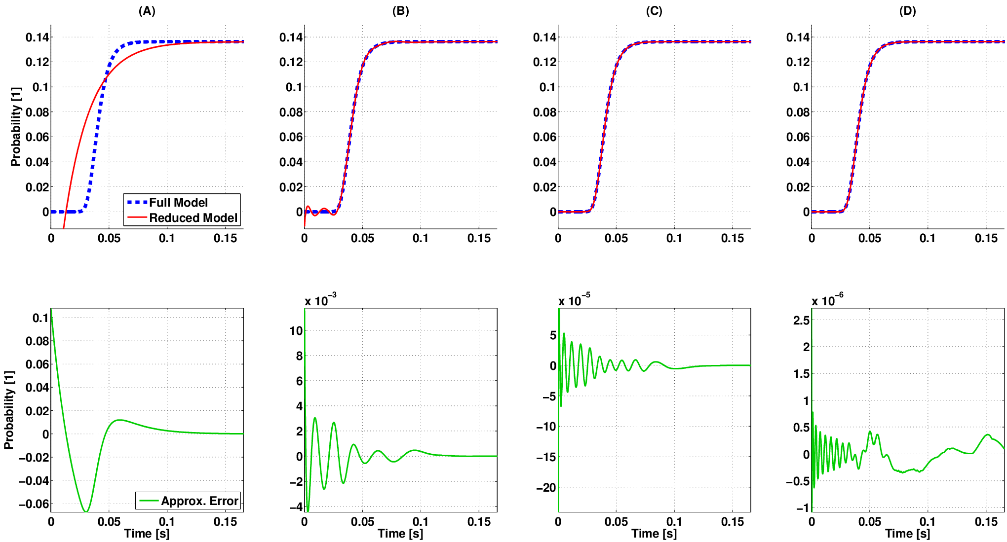
We depict the impact of the number of states on the error of approximation, in Figure 2. There, we note that a very coarse approximation is achieved when we try to approximate the full model with $301$ states with a model of only $1$ state (see the lower panel of Figure 2(A)). In turn, when the reduced order model has $10$ states, the error of approximation is of order $10^{-5}$ , as depicted in the lower panel of Figure 2(C). Furthermore, if the reduced model has $15$ states, the approximation error might already range in the order of the integration error, as suggested by the irregular fluctuations shown in the lower panel of Figure 2(D).

To finalise this section, we note that $\mathcal{L}_{2}$ gain of the approximation error is $427.4607\times 10^{-3},~33.1963\times 10^{-3},~587.9172\times 10^{-6},$ and $6.0955\times 10^{-6}$ , for the reduced models with $1$ , $5$ , $10$ , and $15$ states, respectively. These bounds were obtained by evaluating Expression (15). We note that this is a theoretical bound and does not account for numerical errors during the integration or computation of the Hankel Singular Values.

In the forthcoming section, we obtain reduced order models for a catalytic substrate conversion, and asses the computational burden required to obtain the reduced order model. In addition, we benchmark the time required for simulating the reduced order model against both the computational load required to simulate the full order model and the Stochastic Simulation Algorithm (SSA).

IV-B Stochastic Michaelis-Menten

In this section, we consider the reaction network

whichrepresentsconversionofasubstrate,S $,toaproduct,$ P $,mediatedbyacatalyticagent,$ E $,whichbindstothesubstratetoformthecomplex$ C $.Inthedeterministiccase,itiscommonpracticetoapproximatethemass-action-basedreactionnetworkin\eqref{Eq:CatFull}viathereaction\begin{aligned} S{}\mathrel{\mathop{\makebox[0.0pt]{\rightarrow\displaystyle}}\limits^{\mkern 5.0muv_{MM}(S)\mkern 9.0mu}}{}P,\end{aligned}withnonlinearreactionrate\lx@equationgroup@subnumbering@begin\begin{aligned} v_{MM}([S])=\frac{v_{max}}{k_{m}+[S]}[S],\end{aligned}where$[\circ]$standsforconcentrationoftheargumentand\begin{aligned} v_{max}:&=k_{\mathrm{f}2}[E]_{T},\\ k_{m}:&=\frac{k_{\mathrm{b}1}+k_{\mathrm{f}2}}{k_{\mathrm{f}1}},\\ [E]_{T}:&=[E](\mathnormal{t})+[C](\mathnormal{t}),\quad\textnormal{for any }\mathnormal{t}\geq 0.\end{aligned}\lx@equationgroup@subnumbering@end Ithasbeenshownthatthedynamicsof\eqref{Eq:CatFull}canbereasonablyapproximatedby\eqref{Eq:CatRed}when\cite[cite]{[\@@bibref{}{segel1989quasi}{}{}]}\begin{aligned} [E]_{T}<<S(0)+k_{m}.\end{aligned}\par However,forcasesinwhichthereactionsin\eqref{Eq:CatFull}arebetterdescribedbyastochasticmodel,itisstillpossibletorepresentthedynamicsof$ S $and$ P $withareactionoftheform\eqref{Eq:CatRed}byusingthepropensity\begin{aligned} a_{MMs}(S)=\frac{v_{max}}{k_{m}+S}S,\end{aligned}wherenow$ S $representsthenumberofmoleculesofthesubstrateand$ v_max,k_m $,and$ E_T $areasin\eqref{Eq:vMM},whilethekineticconstantsarethoseofthestochasticmodel.Thisrepresentationisvalidunderthecondition\eqref{Eq:ConMM},asisalsotrueforthedeterministiccase\cite[cite]{[\@@bibref{}{sanft2011legitimacy}{}{}]}.Additionally,thecasewhen\begin{aligned} k_{\mathrm{b}1}>>k_{\mathrm{f}2},\end{aligned}inwhichanonlinearpropensityfunctioncanbeusedtorepresent\eqref{Eq:CatFull}via\eqref{Eq:CatRed}wasconsideredin\cite[cite]{[\@@bibref{}{sanft2011legitimacy}{}{}]}.There,thecondition$ $k_{\mathrm{b}1}$ ¿¿ $k_{\mathrm{f}2}$ $inducesatime-scaleseparationwhichisfurtherusedtoabridgethereactionnetwork\eqref{Eq:CatFull}.Inthefollowing,wewillrefertotherepresentationofthereactionnetwork\eqref{Eq:CatFull}via\eqref{Eq:CatRed}withthepropensityin\eqref{Eq:NlProp}orthatin\cite[cite]{[\@@bibref{}{sanft2011legitimacy}{}{}]}as\textit{stochastic Michaelis-Menten}representation.\par WenowobtainareducedordermodelthatapproximatestheprobabilityofbeinginselectedstatesoftheunderlyingMarkovchain.WederivethisreducedmodelbymeansoftheproceduredescribedinSection\ref{Sec:OrderRed}.Incontrasttotheapproachesin\cite[cite]{[\@@bibref{}{sanft2011legitimacy}{}{}]}andreferencestherein,wedonotassumeanyparticularrelationamongtheparametersandinitialconditions,soourmethodologyismorewidelyapplicable.\par Anotherdifferencefromtheapproachesin\cite[cite]{[\@@bibref{}{sanft2011legitimacy}{}{}]}isthattheyprovetheapplicabilityofSSAalgorithmswiththestochasticMichaelis-Mentenpropensity.Incontrast,wederiveadynamicalsystemthatapproximatesthesolutionoftheCMEwithan\emph{apriori}errorboundgivenby\eqref{Eq:ErrorBound}.Werecallthatinthelimit,theprobabilitydistributionobtainedfromtheSSAtrajectorieswillconvergetothesolutionoftheCME.However,dependingonthekineticparametersandnetworkanalysed,theSSAmightrequirelargecomputationaltimestoprovideresultswiththedesiredaccuracy.\par Itisnoteworthythatevenwhen\eqref{Eq:CatFull}canberepresentedby\eqref{Eq:CatRed},onecanstillobtainareducedmodelviathebalancedmodelreductiondescribedintheSection\ref{Sec:OrderRed},aswedonotassumeanyrelationshipamongtheparametersandinitialconditions.\par Toexemplifytheconceptsabove,wedepictinFigure\ref{Fig:ReductionMM}acomparisonof\begin{inparaenum}\inline@enumerate@item the solution of the CME of \eqref{Eq:CatFull} with propensities shown in Table \ref{Tb:Prope}; \inline@enumerate@item the solution of the CME of the stochastic Michaelis-Menten in \eqref{Eq:CatRed} with the nonlinear propensity in \eqref{Eq:NlProp}; and \inline@enumerate@item the solution of the reduced model described in Section \ref{Sec:OrderRed} for the last state of the Markov chain, which represents total conversion of the substrate to product. \end{inparaenum}Theparametersusedare$ { $k_{\mathrm{f}1}$ , $k_{\mathrm{f}2}$ , $k_{\mathrm{b}1}$ } = {1 [( molecules s )^-1],1 [s ^-1],1 [s ^-1]} $and10initialmoleculesofsubstrate.Withtheseparameters,themethodproposedin\cite[cite]{[\@@bibref{}{sanft2011legitimacy}{}{}]}wouldnotyieldaccurateresults,asthecondition\eqref{Eq:ConMM2}isnotfulfilled($ $k_{\mathrm{b}1}$ = $k_{\mathrm{f}2}$ $).\par TheonlydifferencebetweentheupperandlowerpanelsinFigure\ref{Fig:ReductionMM}isthenumberofinitialmoleculesconsideredfortheenzyme.Intheupperpanelweconsidered1moleculeoftheenzyme,hencecondition\eqref{Eq:ConMM}isfulfilled,andthestochasticMichaelis-Mentenrepresentationmaybeusedtoapproximatethefullmodel.Moreover,onecanusethestochasticMichaelis-Mententoderiveareducedmodelviabalancedrealisation,ascomparedintheupperpaneloftheupperpanelofFigure\ref{Fig:ReductionMM}\textbf{(C)}.There,weapproximatedthestochasticMichaelis-Mentenmodelof$ 11 $stateswithareducedordermodelwith$ 6 $states;the$ L_2 $gainoftheapproximationerrorislessthan$ 0.2807 ×10^-3 $asgivenby\eqref{Eq:ErrorBound}.Incontrast,whenweconsider$ 10 $moleculesofenzymeinitially,condition\eqref{Eq:ConMM}isviolated(as$ E(0) = S(0) $)andthestochasticMichaelis-Mentenmodeldoesnotreproducethedynamicsofthefullreactionnetworkin\eqref{Eq:CatFull},asdepictedinthelowerpanelsofFigure\ref{Fig:ReductionMM}.Wenote,however,thatwecanstillobtainareducedmodelviabalancedrealisationthataccuratelyapproximatesthedynamicsofthefullmodel(cfr.Figure\ref{Fig:ReductionMM}\textbf{(C)}lower).Thereweapproximatedthefullmodelwith$ 66 $statesbyareducedmodelof$ 6 $states,whoseapproximationerror$ L_2 $gainislessthat$ 0.21547×10^-3 $.\par\begin{figure*}\centering\includegraphics[angle={0},width=345.0pt]{ReductionMM.eps} \@@toccaption{{\lx@tag[ ]{{3}}{Validity of the Michaelis-Menten propensity as an approximation of a catalytic substrate conversion. Column {(A)} shows the simulation of the CME associated to \eqref{Eq:CatFull}, where each tread represents the probability of being in every state of the Markov chain; in turn, column {(B)} shows the solution of the CME of \eqref{Eq:CatRed} by using the nonlinear propensity function \eqref{Eq:NlProp}; whereas, column {(C)} shows the probability of being in the last state of the Markov chain, which represents total conversion of the substrate to the product. This probability is obtained via the CME of the full stochastic model, by the CME of reduced Michaelis-Menten stochastic model, and by the approximated model to the CME via balanced realisation. The parameters used for obtaining the numerical solution are $\{k_{\mathrm{f}1},k_{\mathrm{f}2},k_{\mathrm{b}1}\}=\{1,1,1\}$ and $10$ initial molecules of substrate. The only difference between the upper and lower panels is the number of enzymes considered: upper panels $1$ molecule, whereas the lower panels, $10$ molecules. Note that in the lower panel the stochastic Michaelis-Menten approximation is not valid, but the approximation via the balanced model truncation is close to the full model.}}}\@@caption{{\lx@tag[: ]{{Fig. 3}}{Validity of the Michaelis-Menten propensity as an approximation of a catalytic substrate conversion. Column {(A)} shows the simulation of the CME associated to \eqref{Eq:CatFull}, where each tread represents the probability of being in every state of the Markov chain; in turn, column {(B)} shows the solution of the CME of \eqref{Eq:CatRed} by using the nonlinear propensity function \eqref{Eq:NlProp}; whereas, column {(C)} shows the probability of being in the last state of the Markov chain, which represents total conversion of the substrate to the product. This probability is obtained via the CME of the full stochastic model, by the CME of reduced Michaelis-Menten stochastic model, and by the approximated model to the CME via balanced realisation. The parameters used for obtaining the numerical solution are $\{k_{\mathrm{f}1},k_{\mathrm{f}2},k_{\mathrm{b}1}\}=\{1,1,1\}$ and $10$ initial molecules of substrate. The only difference between the upper and lower panels is the number of enzymes considered: upper panels $1$ molecule, whereas the lower panels, $10$ molecules. Note that in the lower panel the stochastic Michaelis-Menten approximation is not valid, but the approximation via the balanced model truncation is close to the full model.}}} \@add@centering\end{figure*}\par NowwefocusonthetimerequiredtosimulatetheCMEandthetimerequiredtosimulatethereducedordermodel.Tocomputethelatter,weneedtoapplysomestatetransformationstotheCME\eqref{Eq:ODEy}toderiveabalancedrealisationthatcanbefurthertruncated.Oncethereducedmodelisobtained,thetimerequiredforitsnumericalsolutionissignificantlysmallercomparedtothetimerequiredforthenumericalsolutionofthefullCME.Toillustratethisreductiononthecomputationaltime,weobtainedtheCMEofthereactionnetwork\eqref{Eq:CatFull}withanequalnumberofmoleculesforthesubstrateandenzymeandzeromoleculesfortherestofthespecies,intheinitialstate;later,weobtainedthereducedordermodelviabalancedrealisation,whichrepresentsthestateoftotalconversionofthesubstratetotheproduct;andcomparedthetimerequiredforobtainingthenumericalsolutionofthefullCME($ $\mathnormal{t}$ _CME $)andthereducedmodel($ $\mathnormal{t}$ _red $)bytheexpression\begin{aligned} \eta=\log_{10}\left(\frac{\mathnormal{t}_{\mathrm{CME}}-\mathnormal{t}_{\mathrm{red}}}{\mathnormal{t}_{\mathrm{red}}}\right).\end{aligned}WedepicttheresultsofthisassessmentinFigure\ref{Fig:Performance}.Thereweobservethatasthenumberofmoleculesfor$ E $and$ S $intheinitialstateincrease,thesavingsonthecomputationaltimerequiredtoobtainthenumericalsolutionofthelower-ordermodelalsoincreases.Wenotethatforthecomparisonin\eqref{Eq:Per}wedidnotaccountforthetimerequiredtoobtainthereducedordermodel.\par\begin{figure*}\centering\includegraphics[angle={0},width=172.5pt]{Performance.eps} \@@toccaption{{\lx@tag[ ]{{4}}{Computational time overhead, as given by \eqref{Eq:Per}, required to solve the full CME (diamonds) and to perform $10^{3}$ SSA runs (squares) as compared to the computational time required in seconds to simulate the reduced order model, as the initial number of molecules for $E$ and $S$ vary from $5$ to $100$. The parameters values used for simulation are identical to those of Figure \ref{Fig:ReductionMM}.}}}\@@caption{{\lx@tag[: ]{{Fig. 4}}{Computational time overhead, as given by \eqref{Eq:Per}, required to solve the full CME (diamonds) and to perform $10^{3}$ SSA runs (squares) as compared to the computational time required in seconds to simulate the reduced order model, as the initial number of molecules for $E$ and $S$ vary from $5$ to $100$. The parameters values used for simulation are identical to those of Figure \ref{Fig:ReductionMM}.}}} \@add@centering\end{figure*}\par Tofinalisethissection,wecomparethecomputationaltimerequiredby\begin{inparaenum}\inline@enumerate@item the derivation of the reduced model via balanced realisation plus the simulation of the reduced model; and \inline@enumerate@item the time required by the FSP \cite[cite]{[\@@bibref{}{Munsky2006}{}{}]} for each time point. \end{inparaenum}WenotethattheFSPobtainsanapproximatedprobabilityvectorwithadesirederrorbound($ ε $)for\textit{one specific time point};hence,ifoneisinterestedinthetransientresponseoftheprobabilitydistribution,onehastoimplementsuchanalgorithmforeverytimestepofinterest.Incontrast,onceoneobtainsthereducedmodelviabalancedrealisationitispossibletousethelower-dimensionalsystemforanynumberoftimepoints.TheseresultsaresummarisedinFigure\ref{Fig:FSPvsBalReal},wherethepanels$ (A),(B) $,and$ (C) $consider$ 10,30 $,and$ 50 $initialmoleculesfor$ E $and$ S $,respectively,andzeromoleculesfortherestofthespecies.TheremainingparametervaluesareidenticaltothoseofFigure\ref{Fig:ReductionMM}.WenotethatfortheFSPthe1-normoftheerrorboundislessthanapredefined$ ε $forthespecifictimepointsofinterest(discretesignal),whereasthe$ L_2 $gainoftheapproximationerror(continuoussignal),obtainedwiththereducedmodelviabalancedrealisation,satisfiestheboundgivenby\eqref{Eq:ErrorBound}.Asthenatureofbotherrorsignalsisdifferent,isdifficulttoperformafaircomparisonofthemethods^{\prime}accuracy.Intheforthcomingsection,weobtainareducedordermodelthatapproximatestheprobabilityofhavingacertainrangeof$ P $molecules.\par\begin{figure*}\centering\includegraphics[angle={0},width=345.0pt]{FSPvsBalReal.eps} \@@toccaption{{\lx@tag[ ]{{5}}{Comparison of the computational time required to obtain the reduced order model via balanced realisation (filled circle) and to obtain the approximative model via the FSP method (empty markers), with different, predefined error bounds ($\varepsilon$). The reaction network analysed is \eqref{Eq:CatFull}. The parameters used for simulation are those of Figure \ref{Fig:ReductionMM}. Panels $\mathbf{(A)}$, $\mathbf{(B)}$, and $\mathbf{(C)}$ consider $10$, $30$, and $50$ initial molecules for $E$ and $S$ and zero molecules for the rest of the species, respectively.}}}\@@caption{{\lx@tag[: ]{{Fig. 5}}{Comparison of the computational time required to obtain the reduced order model via balanced realisation (filled circle) and to obtain the approximative model via the FSP method (empty markers), with different, predefined error bounds ($\varepsilon$). The reaction network analysed is \eqref{Eq:CatFull}. The parameters used for simulation are those of Figure \ref{Fig:ReductionMM}. Panels $\mathbf{(A)}$, $\mathbf{(B)}$, and $\mathbf{(C)}$ consider $10$, $30$, and $50$ initial molecules for $E$ and $S$ and zero molecules for the rest of the species, respectively.}}} \@add@centering\end{figure*}\par$

IV-C Probability for Ranges of Molecules Counts

Up to now, we have obtained reduced models that approximate the probability of being in one state of the Markov chain. In this section, we revisit the reaction network in (IV-B) by obtaining the probability of having a certain number of molecules within predefined ranges. Here we consider the following parameter definitions: $\{k_{\mathrm{f}1},k_{\mathrm{f}2},k_{\mathrm{b}1}\}=\{1,1,1\}$ , $100$ initial molecules of substrate, $100$ initial molecules of enzyme, and zero initial molecules for the rest of the species. By denoting the number of $P$ molecules with $c_{P}$ , we can formulate our problem as approximating the following probabilities

\displaystyle\mathbf{y}(\mathnormal{t})=\begin{pmatrix}\Pr(0\leq c_{P}(\mathnormal{t})\leq 30)\\ \Pr(31<c_{P}(\mathnormal{t})\leq 70)\\ \Pr(71<c_{P}(\mathnormal{t})\leq 100)\end{pmatrix}.

(31)

To derive the CME, one needs to obtain and label all the possible combinations of species molecular counts $\mathbf{s}^{i}$ and organise them in the set $\mathbf{S}$ in (1). Then we have to evaluate the infinitesimal generator $\mathcal{A}$ as in (11) with the corresponding reaction propensities of (IV-B) (see Table I). To obtain an expression for $\mathbf{y}(\mathnormal{t})$ , we need to define the matrix $\mathcal{C}$ in (16b) so that the product of the first row of $\mathcal{C}$ by the vector $\mathbf{p}(\mathnormal{t})$ yield the sum of the probability of all the states $\mathbf{s}^{i}$ such that $c_{P}$ is within the range $[0,30]$ . The next two rows of $\mathcal{C}$ are defined likewise, but accounting for the ranges $c_{P}$ described in the second and third entries of (31). The CME for this system, parameters, and initial number of molecules has $5151$ states. By applying the model reduction technique in Section III, we can approximate the probabilities in (31) by a dynamical system with $16$ states, whose output is depicted in Figure 6. The $\mathcal{L}_{2}$ gain of the approximation error is less than $6.384\times 10^{-3}$ , as estimated by (15).

V Concluding Remarks

In this paper we addressed the order reduction of the infinitesimal generator of a homogeneous, continuous-time, finite and discrete state-space Markov Chain via the reduction of its balanced realisation. Although the application range of these dynamical systems is broad, here we focus on its use on stochastic chemical reaction networks, without loss of generality. In this context, the infinitesimal generator of the Markov chain that describes the probability of having a particular species molecular count is a large set of ODEs.

To reduce the order of the infinitesimal generator of a Markov chain, we used an alternative coordinate system to represent the Chemical Master Equation (CME). This representation, denoted as Lyapunov balanced realisation, has interesting property that the states are organized in decreasing order according to the probabilities of interest. Hence, an accurate approximation can be obtained, for example, by neglecting the last states of the Lyapunov balanced model, as discussed in Section III. Although one may focus on particular states of the Markov chain, it is also possible to account for marginal probability distributions such as in the case study in Section IV-C, or even mean values, by properly defining the matrix $\mathcal{C}$ in (16b).

In many cases, only selected states of the Markov chain might be of practical relevance. For instance, this is the case when facing limited or inexact measurement data, or when only a few states are relevant for downstream signalling in biochemical reactions. Also, in imaging analysis of chemical reaction networks, obtaining the exact count of intracellular protein reporters might be challenging due to limited resolution. Hence, the validation of the mathematical model that describes the process under observation should yield the probability of having an specific range of molecules count of the observed species. We presented this procedure in Section IV-C, for a very simple reaction network. Even in such a simple case, the associated Markov chain presented approximately 5000 distinct states of the system. This highlights how simulation of a system, even in the simplest cases, might imply a computationally intensive task. To alleviate such a burden, the model reduction via balanced realisation used in this paper yields lower-dimensional ODE sets, whose numerical solution might be several orders of magnitude quicker than the numerical solution of the original CME. Moreover, the method used to derive the lower dimensional model provides an upper bound on the approximation error, depending on the number of states neglected to derive the approximation.

Of note, the processes required for deriving the reduced order model itself might take longer computations times compared to the mere simulation of the CME. Nevertheless, the numerical solution of the reduced model might be obtained orders of magnitude faster, depending on the number of molecules of the system, as shown in Figure . Hence, there will be real savings on the computational time when the reduced model is repeatedly utilised, for instance when adopting different initial probability distributions. We would like to stress that to obtain a reduced order model, we have to fix kinetic parameters and to define which are the states of interest. Should we require to modify either of them, a new reduced model has to be derived. Likewise, all methods that require computational calculations, such as the FSP, SSA, and numerical solution of the CME will require numeric values for the parameters and, moreover, specific numerical values for the initial probability distribution. When either of them are modified, a new numerical solution has to be obtained. Additionally, the reduction and simulation of the CME might be orders of magnitude faster than the application of the FSP method, as suggested by the example analysed in Section IV-B.

Another possible use for the reduced model is to derive closed-form expressions of its solution (see [19], for instance), thereby avoiding the need for numerical solution of the reduced ODE set. When the number of states of the Markov chain to reduce is so large that using only one computer is unfeasible, we suggest the use of parallel algorithms to obtain the model reduction by truncation (see e.g. [31, 25])

It is important to note that the reduced order model might lack some properties of the full model. For instance, the infinitesimal generator of the Markov chains studied here describes a positive system: the value of the probabilities will be always positive. However, the reduced order model obtained by truncation used in this paper will not, in general, preserve such a property. This implies that if most of the states of the balanced realisation are neglected to obtain the reduced model, there is a risk of having small, negative values for the approximated probabilities. An example of such phenomenon can be observed on the upper panels of Figure 2(A,B). This suggests the existence of a trade-off on the order and the accuracy of the reduced-order model. As a rule of thumb, a good approximation can be obtained by neglecting those states associated to Hankel Singular Values which are three orders of magnitudes smaller than the largest one. If the possibility of small, negative values for the probability cannot be afforded for the application of the reduced order model, there are other model order reduction methods that preserve the positivity of the original model, such as the recent works [32, 33, 34]. However, it is equally important to note that these approaches are not generally applicable; are more time consuming; and have larger error bounds.

Along this paper, we have considered that the set $\mathbf{S}$ in (1) has all the possible states of the Markov chain under consideration. However, when the number of states is prohibitively large, it is possible to consider a truncation of the set $\mathbf{S}$ ; thereby, obtaining smaller Master Equations. This truncation has two implications:

i) the Master Equation derived from the truncated

\mathbf{S}

will not capture the full probability density function of the Markov chain, but will only focus on the probability of being in those states of interest as characterised in [8]; and ii) the set of ODEs arising from the truncated

\mathbf{S}

will not have the properties in (17).

Hence the change of coordinates in (20) is not necessary, and balanced model reduction can be applied directly to the set of ODEs obtained from the truncated $\mathbf{S}$ . This, in turn, implies that those methods that depend on the truncation of the set $\mathbf{S}$ to derive approximated probability distributions, such as [8], do not antagonise with the model reduction via balanced realisation used in this paper, as both approaches can be complementary.

Appendix A Bound on the Approximation Error of the Model Reduction via Balanced Realisation

Here, we provide some definitions and the derivation of the approximation error bound (15) that arises from the model reduction via balanced realisation described in Section III. The material of this section is based on the Refs. [5, 7].

First, to asses the size of the error of approximation, let us define the $\mathcal{L}_{2}$ norm of a real, time-dependent vector $\mathbf{u}(\mathnormal{t})$ as

\displaystyle||\mathbf{u}||_{\mathcal{L}_{2}}:=\int_{0}^{\tau}\mathbf{u}^{T}(\mathnormal{t})\mathbf{u}(\mathnormal{t})\mathrm{d}t.

When $\tau<\infty$ , one obtains the norm of the truncated signal $\mathbf{u}(\mathnormal{t})$ . To increase readability, we will not explicitly show the upper limit of integration in the norm’s subscript.

Now, in the frequency domain, the linear ODE (12) becomes the following algebraic equation

\mathbf{Y}(\xi)=\mathbf{G}(\xi)\mathbf{U}(\xi),

(32)

where $\xi$ is the complex frequency variable that arises from the Laplace transform of (12), and

\mathbf{G}(\xi):=\mathbf{D}+\mathbf{C}\left(\xi\mathbf{I-A}\right)^{-1}\mathbf{B}.

The complex matrix $\mathbf{G}(\xi)$ is denoted as the transfer function of the system (12) and characterises its input-output behaviour. The $\mathcal{H}_{\infty}$ norm of the complex matrix $\mathbf{G}(\xi)$ is defined as

||\mathbf{G}||_{\mathcal{H}_{\infty}}:=\mathrm{sup}_{\mathrm{Re}(\xi)>0}\sqrt{\bar{\lambda}\left(\mathbf{G}^{*}(\xi)\mathbf{G}(\xi)\right)}.

Here $\bar{\lambda}\left(\circ\right)$ denotes the largest eigenvalue of the argument. In turn, the $\mathcal{H}_{2}$ norm of $\mathbf{G}(\xi)$ , for analytic matrices on the open right half-plane, is

||\mathbf{U}||_{\mathcal{H}_{2}}=\frac{1}{2\pi}\int_{-\infty}^{\infty}\mathrm{Trace}\left(\mathbf{Y(\mathnormal{j}\omega)^{*}Y(\mathnormal{j}\omega)}\right)\mathrm{d}\omega.

When $\mathbf{U}(\xi)$ in (32) belongs to the Banach space endowed of the norm $\mathcal{H}_{2}$ , Theorem 4.4 in [5] states that

\displaystyle||\mathbf{Y}||_{\mathcal{H}_{2}}^{2}=||\mathbf{G}||_{\mathcal{H}_{\infty}}^{2}||\mathbf{U}||_{\mathcal{H}_{2}}^{2}.

(33)

In order to relate the frequency-domain norms with the time-domain norms, we note that the Laplace transform used to obtain the transfer function of (12) is an isomeric isomorphism between the $\mathcal{H}_{2}$ space in the frequency-domain and the $\mathcal{L}_{2}$ space in the time-domain. Thus, from (33), we can infer that

\displaystyle||\mathbf{y}||_{\mathcal{L}_{2}}^{2}=||\mathbf{G}||_{\mathcal{H}_{\infty}}^{2}||\mathbf{u}||_{\mathcal{L}_{2}}^{2}.

(34)

Now, we are ready to present the error bound due to the model-order reduction as presented in [7, Th. 11.1]

Theorem A.1

Let $\mathbf{G}(\xi)$ be a stable rational transfer function with Hankel singular values $\sigma_{1}\geq\sigma_{2}\geq...\geq\sigma_{w}$ and let $\mathbf{G}_{\mathrm{red}}(\xi)$ be obtained by truncating or residualising the balanced realization of $\mathbf{G}(\xi)$ to the first $k$ states. Then

||\mathbf{G}-\mathbf{G}_{\mathrm{red}}||_{\mathcal{H}_{\infty}}\leq 2\sum_{i=k+1}^{w}\sigma_{i}.

(35)

Hence, the relationship in (34) implies

\displaystyle\frac{\left|\left|\mathbf{y}-\mathbf{y}_{\textrm{red}}\right|\right|_{\mathcal{L}_{2}}}{\left|\left|\mathbf{u}\right|\right|_{\mathcal{L}_{2}}}\leq 2\sum_{i=k+1}^{w}\sigma_{i}.

(15)

References

[1] W. Feller, An introduction to probability theory and its applications, 3rd ed. John Wiley & Sons, 1968, vol. 1.
[2] P. Bremaud, Markov chains: Gibbs fields, Monte Carlo simulation, and queues. springer, 1999, vol. 31.
[3] N. G. Van Kampen, Stochastic processes in physics and chemistry, 3rd ed. North-Holland Personal Library, 2007, vol. 1.
[4] B. Moore, “Principal component analysis in linear systems: Controllability, observability, and model reduction,” Automatic Control, IEEE Transactions on, vol. 26, no. 1, pp. 17–32, 1981.
[5] K. Zhou, J. C. Doyle, and Glover, Robust and optimal control. Prentice Hall New Jersey, 1996, vol. 40.
[6] S. Gugercin and A. C. Antoulas, “A survey of model reduction by balanced truncation and some new results,” International Journal of Control, vol. 77, no. 8, pp. 748–766, 2004.
[7] S. Skogestad and I. Postlethwaite, Multivariable feedback control: analysis and design. Wiley New York, 2007, vol. 2.
[8] B. Munsky and M. Khammash, “The finite state projection algorithm for the solution of the chemical master equation,” The Journal of Chemical Physics, vol. 124, no. 4, p. 044104, 2006.
[9] Y. Saad, “Analysis of some krylov subspace approximations to the matrix exponential operator,” SIAM Journal on Numerical Analysis, vol. 29, no. 1, pp. 209–228, 1992.
[10] K. Burrage, M. Hegland, S. Macnamara, and R. B. Sidje, “A krylov-based finite state projection algorithm for solving the chemical master equation arising in the discrete modelling of biological systems,” in Proceedings of the Markov 150th Anniversary Conference. Boson Books, Raleigh, NC, 2006, pp. 21–38.
[11] S. Menz, J. C. Latorre, C. Schütte, and W. Huisinga, “Hybrid stochastic–deterministic solution of the chemical master equation,” Multiscale Modeling & Simulation, vol. 10, no. 4, pp. 1232–1262, 2012.
[12] E. L. Haseltine and J. B. Rawlings, “Approximate simulation of coupled fast and slow reactions for stochastic chemical kinetics,” The Journal of chemical physics, vol. 117, p. 6959, 2002.
[13] T. Jahnke, “On reduced models for the chemical master equation,” Multiscale Modeling & Simulation, vol. 9, no. 4, pp. 1646–1676, 2011.
[14] M. Barrio, K. Burrage, P. Burrage, A. Leier, and T. Marquez-Lago, “Computational approaches for modelling intrinsic noise and delays in genetic regulatory networks,” in Handbook of Research on Computational Methodologies in Gene Regulatory Networks, S. Das, D. Caragea, S. Welch, and W. H. Hsu, Eds. Hershey PA: IGI Global, 2010, pp. 169–197.
[15] M. Ullah and O. Wolkenhauer, Stochastic approaches for systems biology. Springer, 2011.
[16] D. T. Gillespie, Y. Cao, K. R. Sanft, and L. R. Petzold, “The subtle business of model reduction for stochastic chemical kinetics,” The Journal of chemical physics, vol. 130, p. 064103, 2009.
[17] M. Barrio, A. Leier, and T. T. Marquez-Lago, “Reduction of chemical reaction networks through delay distributions,” The Journal of chemical physics, vol. 138, p. 104114, 2013.
[18] A. Leier, M. Barrio, and T. T. Marquez-Lago, 2013, submited.
[19] F. López-Caamal and T. T. Marquez-Lago, “Exact probability distributions of selected species in stochastic chemical reaction networks,” 2013, submitted.
[20] C. Lee and P. Kim, “An analytical approach to solutions of master equations for stochastic nonlinear reactions,” Journal of Mathematical Chemistry, vol. 50, no. 6, pp. 1550–1569, 2012.
[21] K. Sanft, D. Gillespie, and L. Petzold, “Legitimacy of the stochastic michaelis-menten approximation,” Systems Biology, IET, vol. 5, no. 1, pp. 58–69, 2011.
[22] L. J. Allen, An introduction to stochastic processes with applications to biology. Pearson Education New Jersey, 2003.
[23] L. Farina and S. Rinaldi, Positive linear systems: Theory and applications. John Wiley & Sons, 2011, vol. 50.
[24] D. T. Gillespie, “A rigorous derivation of the chemical master equation,” Physica A: Statistical Mechanics and its Applications, vol. 188, no. 1, pp. 404–425, 1992.
[25] P. Benner and E. S. Quintana-Ortí, Model reduction based on spectral projection methods. Springer, 2005.
[26] C.-T. Chen, Linear system theory and design. Oxford University Press, Inc., 1998.
[27] C. P. Therapos, “Balancing transformations for unstable nonminimal linear systems,” Automatic Control, IEEE Transactions on, vol. 34, no. 4, pp. 455–457, 1989.
[28] L. Pernebo and L. Silverman, “Model reduction via balanced state space representations,” Automatic Control, IEEE Transactions on, vol. 27, no. 2, pp. 382–387, 1982.
[29] R. E. Kalman, “Mathematical description of linear dynamical systems,” Journal of the Society for Industrial & Applied Mathematics, Series A: Control, vol. 1, no. 2, pp. 152–192, 1963.
[30] L. A. Segel and M. Slemrod, “The quasi-steady-state assumption: a case study in perturbation,” SIAM review, vol. 31, no. 3, pp. 446–477, 1989.
[31] J. M. Badía, P. Benner, R. Mayo, and E. S. Quintana-Ortí, “Parallel algorithms for balanced truncation model reduction of sparse systems,” in Applied Parallel Computing. State of the Art in Scientific Computing. Springer, 2006, pp. 267–275.
[32] J.-e. Feng, J. Lam, Z. Shu, and Q. Wang, “Internal positivity preserved model reduction,” International Journal of Control, vol. 83, no. 3, pp. 575–584, 2010.
[33] P. Li, J. Lam, Z. Wang, and P. Date, “Positivity-preserving h∞ model reduction for positive systems,” Automatica, vol. 47, no. 7, pp. 1504–1511, 2011.
[34] C. Grussler and T. Damm, “A symmetry approach for balanced truncation of positive linear systems,” in Decision and Control (CDC), 2012 IEEE 51st Annual Conference on. IEEE, 2012, pp. 4308–4313.