Decentralized Optimal Dispatch of Photovoltaic Inverters in Residential Distribution SystemsThanks: Submitted March 5, 2013; revised July 23, 2014; accepted September 4, 2014. This work was supported by NSF-CCF grants no. 1423316 and CyberSEES 1442686, the Institute of Renewable Energy and the Environment (IREE) grant no. RL-0010-13, University of Minnesota, and by the Laboratory Directed Research and Development (LDRD) Program at the National Renewable Energy Laboratory. E. Dall’Anese, S. Dhople, and G. Giannakis are with the Dept. of ECE and Digital Technology Center, University of Minnesota, 200 Union Street SE, Minneapolis, MN, USA; e-mails: {emiliano, sdhople, georgios}@umn.edu. B. Johnson is with the National Renewable Energy Laboratory, Golden, CO, USA; e-mail: brian.johnson@nrel.gov
Abstract
Decentralized methods for computing optimal real and reactive power setpoints for residential photovoltaic (PV) inverters are developed in this paper. It is known that conventional PV inverter controllers, which are designed to extract maximum power at unity power factor, cannot address secondary performance objectives such as voltage regulation and network loss minimization. Optimal power flow techniques can be utilized to select which inverters will provide ancillary services, and to compute their optimal real and reactive power setpoints according to well-defined performance criteria and economic objectives. Leveraging advances in sparsity-promoting regularization techniques and semidefinite relaxation, this paper shows how such problems can be solved with reduced computational burden and optimality guarantees. To enable large-scale implementation, a novel algorithmic framework is introduced — based on the so-called alternating direction method of multipliers — by which optimal power flow-type problems in this setting can be systematically decomposed into sub-problems that can be solved in a decentralized fashion by the utility and customer-owned PV systems with limited exchanges of information. Since the computational burden is shared among multiple devices and the requirement of all-to-all communication can be circumvented, the proposed optimization approach scales favorably to large distribution networks.
Index Terms:
Alternating direction method of multipliers, decentralized optimization, distribution systems, optimal power flow, photovoltaic systems, sparsity, voltage regulation.I Introduction
THE proliferation of residential-scale photovoltaic (PV) systems has highlighted unique challenges and concerns in the operation and control of low-voltage distribution networks. Secondary-level control of PV inverters can alleviate extenuating circumstances such as overvoltages during periods when PV generation exceeds the household demand, and voltage transients during rapidly varying atmospheric conditions [1]. Initiatives to upgrade inverter controls and develop business models for ancillary services are currently underway in order to facilitate large-scale integration of renewables while ensuring reliable operation of existing distribution feeders [2].
Examples of ancillary services include reactive power compensation, which has been recognized as a viable option to effect voltage regulation at the medium-voltage distribution level [3, 4, 5, 6, 7]. The amount of reactive power injected or absorbed by inverters can be computed based on either local droop-type proportional laws [3, 5], or optimal power flow (OPF) strategies [6, 7]. Either way, voltage regulation with this approach comes at the expense of low power factors at the substation and high network currents, with the latter leading to high power losses in the network [8]. Alternative approaches require inverters to operate at unity power factor and to curtail part of the available active power [8, 9]. For instance, heuristics based on droop-type laws are developed in [8] to compute the active power curtailed by each inverter in a residential system. Active power curtailment strategies are particularly effective in the low-voltage portion of distribution feeders, where the high resistance-to-inductance ratio of low-voltage overhead lines renders voltage magnitudes more sensitive to variations in the active power injections [10].
Recently, we proposed an optimal inverter dispatch (OID) framework [11] where the subset of critical PV-inverters that most strongly impact network performance objectives are identified and their real and reactive power setpoints are computed. This is accomplished by formulating an OPF-type problem, which encapsulates well-defined performance criteria as well as network and inverter operational constraints. By leveraging advances in sparsity-promoting regularizations and semidefinite relaxation (SDR) techniques [11], the problem is then solved by a centralized computational device with reduced computational burden. The proposed OID framework provides increased flexibility over Volt/VAR approaches [3, 5, 6, 7] and active power curtailment methods [8, 9] by: i) determining in real-time those inverters that must participate in ancillary services provisioning; and, ii) jointly optimizing both the real and reactive power produced by the participating inverters (see, e.g., Figs. 3 (c)-(d) for an illustration of the the inverters’ operating regions under OID).
As proposed originally, the OID task can be carried out on a centralized computational device which has to communicate with all inverters. In this paper, the OID problem proposed in [11] is strategically decomposed into sub-problems that can be solved in a decentralized fashion by the utility-owned energy managers and customer-owned PV systems, with limited exchanges of information. Hereafter, this suite of decentralized optimization algorithms is referred to as decentralized optimal inverter dispatch (DOID). Building on the concept of leveraging both real and reactive power optimization [11], and decentralized solution approaches for OPF problems [12], two novel decentralized approaches are developed in this paper. In the first setup, all customer-owned PV inverters can communicate with the utility. The utility optimizes network performance (quantified in terms of, e.g., power losses and voltage regulation) while individual customers maximize their economic objectives (quantified in terms of, e.g., the amount of active power they might have to curtail). This setup provides flexibility to the customers to specify their optimization objectives since the utility has no control on customer preferences. In the spirit of the advanced metering infrastructure (AMI) paradigm, utility and customer-owned EMUs exchange relevant information [13, 14] to agree on the optimal PV-inverter setpoints. Once the decentralized algorithms have converged, the active and reactive setpoints are implemented by the inverter controllers. In the second DOID approach, the distribution network is partitioned into clusters, each of which contains a set of customer-owned PV inverters and a single cluster energy manager (CEM). A decentralized algorithm is then formulated such that the operation of each cluster is optimized and with a limited exchange of voltage-related messages, the interconnected clusters consent on the system-wide voltage profile. The decentralized OID frameworks are developed by leveraging the alternating direction method of multipliers (ADMM) [15, 16].
Related works include [17], where augmented Lagrangian methods (related to ADMM) were employed to decompose non-convex OPF problems for transmission systems into per-area instances, and [18, 19], where standard Lagrangian approaches were utilized in conjunction with Newton methods. ADMM was utilized in [20] to solve non-convex OPF renditions in a decentralized fashion, and in [21], where successive convex approximation methods were utilized to deal with nonconvex costs and constraints. In the distribution systems context, semidefinite relaxations of the OPF problem for balanced systems were developed in [22], and solved via node-to-node message passing by using dual (sub-)gradient ascent-based schemes. Similar message passing is involved in the ADMM-based decentralized algorithm proposed in [4] where a reactive power compensation problem based on approximate power flow models is solved. SDR of the OPF task in three-phase unbalanced systems was developed in [12]; the resultant semidefinite program was solved in a distributed fashion by using ADMM.

The decentralized OID framework considerably broadens the setups of [17, 18, 19, 20, 21, 12, 22] by accommodating different message passing strategies that are relevant in a variety of practical scenarios (e.g., customer-to-utility, customer-to-CEM and CEM-to-CEM communications). The proposed decentralized schemes offer improved optimality guarantees over [17, 18, 19, 20], since it is grounded on an SDR technique; furthermore, ADMM enables superior convergence compared to [22]. Finally, different from the distributed reactive compensation strategy of [4], the proposed framework considers the utilization of an exact AC power flow model, as well as a joint computation of active and reactive power setpoint.
For completeness, ADMM was utilized also in [23, 24] for decentralized multi-area state estimation in transmission systems, and in [25] to distribute over geographical areas the distribution system reconfiguration task.
The remainder of the paper is organized as follows. Section II briefly outlines the centralized OID problem proposed in [11]. Sections III and IV describe the two DOID problems discussed above. Case studies to validate the approach are presented in Section V. Finally, concluding remarks and directions for future work are presented in Section VI.
Notation: Upper-case (lower-case) boldface letters will be used for matrices (column vectors); for transposition; complex-conjugate; and, complex-conjugate transposition; and denote the real and imaginary parts of a complex number, respectively; the imaginary unit. the matrix trace; the matrix rank; denotes the magnitude of a number or the cardinality of a set; ; ; and stands for the Frobenius norm. Given a given matrix , denotes its -th entry. Finally, denotes the identity matrix; and, , the matrices with all zeroes and ones, respectively.
II Centralized optimal inverter dispatch
II-A Network and PV-inverter models
Consider a distribution system comprising nodes collected in the set (node denotes the secondary of the step-down transformer), and lines represented by the set of edges . For simplicity of exposition, a balanced system is considered; however, both the centralized and decentralized frameworks proposed subsequently can be extended to unbalanced systems following the methods in [12]. Subsets collect nodes corresponding to utility poles (with zero power injected or consumed), and those with installed residential PV inverters, respectively (see Fig. 1).

Let and denote the phasors for the line-to-ground voltage and the current injected at node , respectively, and define and . Using Ohm’s and Kirchhoff’s circuit laws, the linear relationship can be established, where the system admittance matrix is formed based on the system topology and the -equivalent circuit of lines , as illustrated in Fig. 2; see also [10, Chapter 6] for additional details on line modeling. Specifically, with and denoting the series and shunt admittances of line , the entries of are defined as
where denotes the set of nodes connected to the -th one through a distribution line.
A constant model [10] is adopted for the load, with and denoting the active and reactive demands at node , respectively. For given solar irradiation conditions, let denote the maximum available active power from the PV array at node . The proposed framework calls for the joint control of both real and reactive power produced by the PV inverters. In particular, the allowed operating regime on the complex-power plane for the PV inverters is illustrated in Fig. 3 (d) and described by
| (1) |
where is the active power curtailed, and is the reactive power injected/absorbed by the inverter at node . Notice that if there is no limit to the power factor, then , and the operating region is given by Fig. 3(c).


II-B Centralized optimization strategy
The centralized OID framework in [11] invokes joint optimization of active and reactive powers generated by the PV inverters, and it offers the flexibility of selecting the subset of critical PV inverters that should be dispatched in order to fulfill optimization objectives and ensure electrical network constraints. To this end, let be a binary variable indicating whether PV inverter provides ancillary services or not and assume that at most PV inverters are allowed to provide ancillary services. Selecting a (possibly time-varying) subset of inverters promotes user fairness [3], prolongs inverter lifetime [3], and captures possible fixed-rate utility-customer pricing/rewarding strategies [2]. Let and collect the active powers curtailed and the reactive powers injected/absorbed by the inverters. With these definitions, the OID problem is formulated as follows:
| (2a) | ||||
| (2b) | ||||
| (2c) | ||||
| (2d) | ||||
| (2g) | ||||
where constraint (2b) is enforced at each node ; is a given cost function capturing both network- and customer-oriented objectives [11, 2]; and, (2)-(2g) jointly indicate which inverters have to operate either under OID (i.e., ), or, in the business-as-usual mode (i.e., ). An alternative problem formulation can be obtained by removing constraint (2g), and adopting the cost in (2a), with a weighting coefficient utilized to trade off achievable cost for the number of controlled inverters. When represents a fixed reward for customers providing ancillary services [2] and models costs associated with active power losses and active power set points, OID (2) returns the inverter setpoints that minimize the economic cost incurred by feeder operation.
As with various OPF-type problem formulations, the power balance and lower bound on the voltage magnitude constraints (2b), (2c) and (2d), respectively, render the OID problem nonconvex, and thus challenging to solve optimally and efficiently. Unique to the OID formulation are the binary optimization variables ; finding the optimal (sub)set of inverters to dispatch involves the solution of combinatorially many subproblems. Nevertheless, a computationally-affordable convex reformulation was developed in [11], by leveraging sparsity-promoting regularization [26] and semidefinite relaxation (SDR) techniques [27, 23, 12] as briefly described next.
In order to bypass binary selection variables, key is to notice that that if inverter is not selected for ancillary services, then one clearly has that [cf. (2)]. Thus, for , one has that the real-valued vector is group sparse [26]; meaning that, either the sub-vectors equal or not [11]. This group-sparsity attribute enables discarding the binary variables and to effect PV inverter selection by regularizing the cost in (2) with the following function:
| (3) |
where is a tuning parameter. Specifically, the number of inverters operating under OID decreases as is increased [26].
Key to developing a relaxation of the OID task is to express powers and voltage magnitudes as linear functions of the outer-product Hermitian matrix , and to reformulate the OID problem with cost and constraints that are linear in , as well as the constraints and [27, 23, 12]. The resultant problem is still nonconvex because of the constraint ; however in the spirit of SDR, this constraint can be dropped.
To this end, define the matrix per node , where denotes the canonical basis of . Based on , define also the Hermitian matrices , , and . Using these matrices, along with (3) the relaxed convex OID problem can be formulated as
| (4a) | ||||
| (4b) | ||||
| (4c) | ||||
| (4d) | ||||
| (4e) | ||||
| (4f) | ||||
If the optimal solution of the relaxed problem (4) has rank 1, then the resultant voltages, currents, and power flows are globally optimal for given inverter setpoints [27]. Sufficient conditions for SDR to be successful in OPF-type problems are available for networks that are radial and balanced in [28, 22], whereas the virtues of SDR for unbalanced medium- and low-voltage distribution systems have been demonstrated in [12]. As for the inverter setpoints , those obtained from (4) may be slightly sub-optimal compared to the setpoints that would have been obtained by solving the optimization problem (2). This is mainly due to the so-called “shrinkage effect” introduced by the regularizer (3) [26]. Unfortunately, a numerical assessment of the optimality gap is impractical, since finding the globally optimal solution of problem (2) under all setups is computationally infeasible.
To solve the OID problem, all customers’ loads and available powers must be gathered at a central processing unit (managed by the utility company), which subsequently dispatches the PV inverter setpoints. Next, decentralized implementations of the OID framework are presented so that the OID problem can be solved in a decentralized fashion with limited exchange of information. From a computational perspective, decentralized schemes ensure scalability of problem complexity with respect to the system size.
III DOID: utility-customer message passing
Consider decoupling the cost in (4a) as , where captures utility-oriented optimization objectives, which may include e.g., power losses in the network and voltage deviations [11, 6, 7]; and, is a convex function modeling the cost incurred by (or the reward associated with) customer when the PV inverter is required to curtail power. Without loss of generality, a quadratic function is adopted here, where the choice of the coefficients is based on specific utility-customer prearrangements [2] or customer preferences [11].
Suppose that customer transmits to the utility company the net active power and the reactive load ; subsequently, customer and utility will agree on the PV-inverter setpoint, based on the optimization objectives described by and . To this end, let and represent copies of , and , respectively, at the utility. The corresponding vectors that collect the copies of the inverter setpoints are denoted by and , respectively. Then, using the additional optimization variables , the relaxed OID problem (4) can be equivalently reformulated as:
| (5a) | ||||
| (5b) | ||||
| (5c) | ||||
| (5d) | ||||
| (5e) | ||||
| (5f) | ||||
| (5g) | ||||
where constraints (5g) ensure that utility and customer agree upon the inverters’ setpoints, and is the regularized cost function to be minimized at the utility.
The consensus constraints (5g) render problems (4) and (5) equivalent; however, the same constraints impede problem decomposability, and thus modern optimization techniques such as distributed (sub-)gradient methods [13, 14] and ADMM [15, Sec. 3.4] cannot be directly applied to solve (5) in a decentralized fashion. To enable problem decomposability, consider introducing the auxiliary variables per inverter . Using these auxiliary variables, (5) can be reformulated as
| (6a) | ||||
| (6b) | ||||
| (6c) | ||||
Problem (6) is equivalent to (4) and (5); however, compared to (4)-(5), it is amenable to a decentralized solution via ADMM [15, Sec. 3.4] as described in the remainder of this section. ADMM is preferred over distributed (sub-)gradient schemes because of its significantly faster convergence [4] and resilience to communication errors [29].
Per inverter , let denote the multipliers associated with the two constraints in (22c), and the ones associated with (22d). Next, consider the partial quadratically-augmented Lagrangian of (6), defined as follows:
| (7) |
where collects the optimization variables of the utility; are the decision variables for customer ; is the set of auxiliary variables; collects the dual variables; and is a given constant. Based on (7), ADMM amounts to iteratively performing the steps [S1]-[S3] described next, where denotes the iteration index:
[S1] Update variables as follows:
| (8) | ||||
Furthermore, per inverter , update as follows:
| (9) | ||||
[S2] Update auxiliary variables :
| (10) |
[S3] Dual update:
| (11a) | ||||
| (11b) | ||||
| (11c) | ||||
| (11d) | ||||
In [S1], the primal variables are obtained by minimizing (7), where the auxiliary variables and the multipliers are kept fixed to their current iteration values. Likewise, the auxiliary variables are updated in [S2] by fixing to their up-to-date values. Finally, the dual variables are updated in [S3] via dual gradient ascent.
It can be noticed that step [S2] favorably decouples into scalar and unconstrained quadratic programs, with and solvable in closed-form. Using this feature, the following lemma can be readily proved.
Lemma 1
Suppose that the multipliers are initialized as . Then, for all iterations , it holds that:
i) ;
ii) .
iii) ; and,
iv) .
Using Lemma 1, the conventional ADMM steps [S1]–[S3] can be simplified as follows.
[S1′] At the utility side, variables are updated by solving the following convex optimization problem:
| (12a) | ||||
| where function is defined as | ||||
| (12b) | ||||
At the customer side, the PV-inverter setpoints are updated by solving the following constrained quadratic program:
| (13) | ||||
[S2′] At the utility and customer sides, the dual variables are updated as:
| (14a) | ||||
| (14b) | ||||

The resultant decentralized algorithm entails a two-way message exchange between the utility and customers of the current iterates and . Specifically, at each iteration , the utility-owned device solves the OID rendition (12) to update the desired PV-inverter setpoints based on the performance objectives described by (which is regularized with the term enforcing consensus with the setpoints computed at the customer side), as well as the electrical network constraints (5b)-(5e); once (12) is solved, the utility relays to each customer a copy of the iterate value . In the meantime, the PV-inverter setpoints are simultaneously updated via (13) and subsequently sent to the utility. Once the updated local iterates are exchanged, utility and customers update the local dual variables (14).
The resultant decentralized algorithm is tabulated as Algorithm 1, illustrated in Fig. 4, and its convergence to the solution of the centralized OID problem (4) is formally stated next.
Proposition 1
Notice that problem (12) can be conveniently reformulated in a standard SDP form (which involves the minimization of a linear function, subject to linear (in)equalities and linear matrix inequalities) by introducing pertinent auxiliary optimization variables and by using the Schur complement [30, 27, 11]. Finally, for a given consensus error , the algorithm terminates when . However, it is worth emphasizing that, at each iteration , the utility company solves a consensus-enforcing regularized OID problem, which yields intermediate voltages and power flows that clearly adhere to electrical network constraints.
Once the decentralized algorithm has converged, the real and reactive setpoints are implemented in the PV inverters. Notice however that Algorithm 1 affords an online implementation; that is, the intermediate PV-inverter setpoints are dispatched (and set at the customer side) as and when they become available, rather than waiting for the algorithm to converge.
IV DOID: Network cluster partitions
Consider the case where the distribution network is partitioned into clusters, with denoting the set of nodes within cluster . Also, define ; that is, also includes the nodes belonging to different clusters that are connected to the -th one by a distribution line [23, 12] (see Fig. 5 for an illustration). Hereafter, superscript will be used to specify quantities pertaining to cluster ; e.g., is the set of houses located within cluster , and vectors collect copies of the setpoints of PV inverters available with the -th CEM [cf. (5)]. With regard to notation, an exception is , which denotes the sub-matrix of corresponding to nodes in the extended cluster .
Based on this network partitioning, consider decoupling the network-related cost in (5a) as
where is the number of clusters, captures optimization objectives of the -th cluster (e.g., power losses within the cluster [17, 12]), and the sparsity-promoting regularization function is used to determine which PV inverters in provide ancillary services. Further, per-cluster , define the region of feasible power flows as [cf. (5b)-(5e)]:
where , and are the sub-matrices of , and , respectively, formed by extracting rows and columns corresponding to nodes in . With these definitions, problem (5) can be equivalently formulated as:
| (20a) | ||||
| (20b) | ||||
| (20c) | ||||
| (20d) | ||||
Notice that, similar to (5g), constraints (20d) ensure that the CEM and customer-owned PV systems consent on the optimal PV-inverter setpoints. Formulation (20) effectively decouples cost, power flow constraints, and PV-related consensus constraints (20d) on a per-cluster basis. The main challenge towards solving (20) in a decentralized fashion lies in the positive semidefinite (PSD) constraint , which clearly couples the matrices . To address this challenge, results on completing partial Hermitian matrices from [31] will be leveraged to identify partitions of the distribution network in clusters for which the PSD constraint on would decouple to , . This decoupling would clearly facilitate the decomposability of (20) in per-cluster sub-problems [23, 12].
Towards this end, first define the set of neighboring clusters for the -th one as . Further, let be a graph capturing the control architecture of the distribution network, where nodes represent the clusters and edges connect neighboring clusters (i.e., based on sets ); for example, the graph associated with the network in Fig. 5 has two nodes, connected through an edge (since the two areas are connected). In general, it is clear that if clusters and are neighbors, then CEM and CEM must agree on the voltages at the two end points of the distribution line connecting the two clusters. For example, with reference to Fig. 5, notice that line connects clusters and . Therefore, CEM 1 and CEM 2 must agree on voltages and . Lastly, let denote the sub-matrix of corresponding to the two voltages on the line connecting clusters and . Recalling the previous example, agreeing on and is tantamount to setting , where is a matrix representing the outer-product . Using these definitions, the following proposition can be proved by suitably adapting the results of [23, 12] to the problem at hand.
Proposition 2
Notice that the matrix is replaced by per-cluster reduced-dimensional matrices in (21). Proposition 2 is grounded on the results of [31], which asserts that a PSD matrix can be obtained starting from sub-matrices if and only if the graph induced by is chordal. Since a PSD matrix can be reconstructed from , it suffices to impose contraints , . Assumptions (i)–(ii) provide sufficient conditions for the graph induced by to be chordal, and they are typically satisfied in practice (e.g., when each cluster is set to be a lateral or a sub-lateral). The second part of the proposition asserts that, for the completable PSD matrix to have rank , all matrices must have rank ; thus, if for all clusters, then represents a globally optimal power flow solution for given inverter setpoints.
Similar to (6), auxiliary variables are introduced to enable decomposability of (21) in per-cluster subproblems. With variables associated with inverter , and with neighboring clusters and , (21) is reformulated as:
| (22a) | ||||
| (22b) | ||||
| (22c) | ||||
| (22d) | ||||
This problem can be solved across clusters by resorting to ADMM. To this end, a partial quadratically-augmented Lagrangian, obtained by dualizing constraints , , , and is defined first; then, the standard ADMM steps involve a cyclic minimization of the resultant Lagrangian with respect to (by keeping the remaining variables fixed); the auxiliary variables ; and, finally, a dual ascent step [15, Sec. 3.4]. It turns out that Lemma 1 still holds in the present case. Thus, using this lemma, along with the result in [12, Lemma 3], it can be shown that the ADMM steps can be simplified as described next (the derivation is omitted due to space limitations):
[S1′′] Each PV system updates the local copy via (13); while, each CEM updates the voltage profile of its cluster, and the local copies of the setpoints of inverters by solving the following convex problem:
| (23a) | ||||
| (23b) | ||||
| where vectors and collect the real and imaginary parts, respectively, of the entries of the matrix ; the regularization function enforcing consensus on the inverter setpoints is defined as in (12b) (but with the summation limited to inverters ) and, is given by: | ||||
| (23g) | ||||
[S2′′] Update dual variables via (14) at both, the customer and the CEMs; variables are updated locally per cluster as:
| (24a) | ||||
| (24b) | ||||

The resultant decentralized algorithm is tabulated as Algorithm 2, illustrated in Fig. 5, and it involves an exchange of: (i) the local submatrices among neighboring CEMs to agree upon the voltages on lines connecting clusters; and, (ii) the local copies of the PV inverter setpoints between the CEM and customer-owned PV systems. Using arguments similar to Proposition 3, convergence of the algorithm can be readily established.
Proposition 3
Once the decentralized algorithm has converged, the real and reactive setpoints are implemented by the PV inverter controllers.
Finally, notice that the worst case complexity of an SDP is on the order for general purpose solvers, with denoting the total number of constraints, the total number of variables, and a given solution accuracy [30]. It follows that the worst case complexity of (23) is markedly lower than the one of the centralized problem (4). Further, the sparsity of and the so-called chordal structure of the underlying electrical graph matrix can be exploited to obtain substantial computational savings; see e.g., [32].
V Case Studies
Consider the distribution network in Fig. 1, which is adopted from [8, 11]. The simulation parameters are set as in [11] to check the consistency between the results of centralized and decentralized schemes. Specifically, the pole-pole distance is set to m; lengths of the drop lines are set to m; and voltage limits are set to 0.917 pu and 1.042 pu, respectively (see e.g., [8]). The optimization package CVX11 1 [Online] Available: http://cvxr.com/cvx/ is employed to solve relevant optimization problems in MATLAB. In all the conducted numerical tests, the rank of matrices and was always , meaning that globally optimal power flow solutions were obtained for given inverter setpoints.
The available active powers are computed using the System Advisor Model (SAM)22 2 [Online] Available at https://sam.nrel.gov/. of the National Renewable Energy Laboratory (NREL); specifically, the typical meteorological year (TMY) data for Minneapolis, MN, during the month of July are used. All 12 houses feature fixed roof-top PV systems, with a dc-ac derating coefficient of . The dc ratings of the houses are as follows: kW for houses ; kW for ; and, kW for the remaining five houses. The active powers generated by the inverters with dc ratings of kW, kW, and kW are plotted in Fig. 6(a). As suggested in [3], it is assumed that the PV inverters are oversized by of the resultant ac rating. The minimum power factor for the inverters is set to 0.85 [33].




The residential load profile is obtained from the Open Energy Info database and the base load experienced in downtown Saint Paul, MN, during the month of July is used for this test case. To generate 12 different load profiles, the base active power profile is perturbed using a Gaussian random variable with zero mean and standard deviation W; the resultant active loads are plotted in Fig. 6(b). To compute the reactive loads , a power factor of 0.9 is presumed [8].
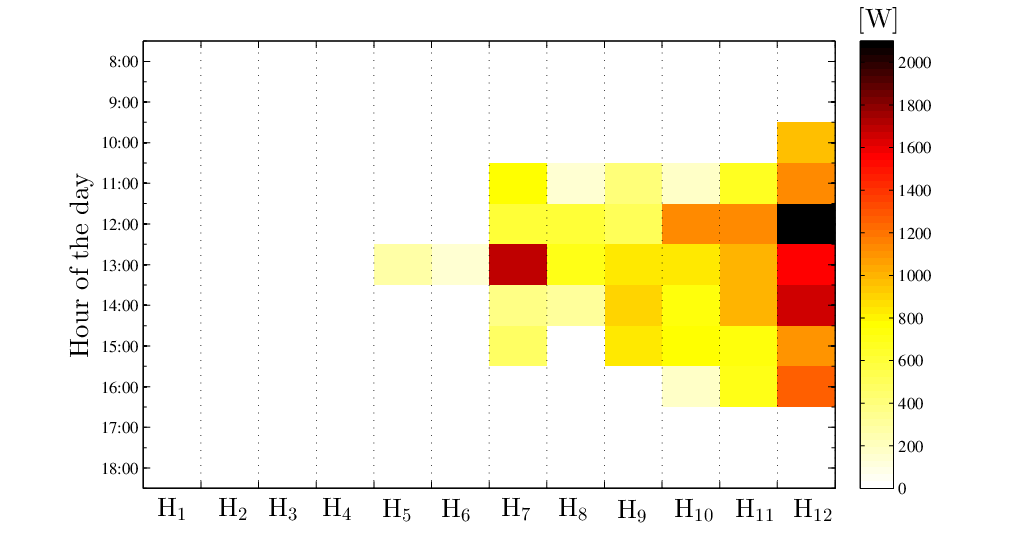
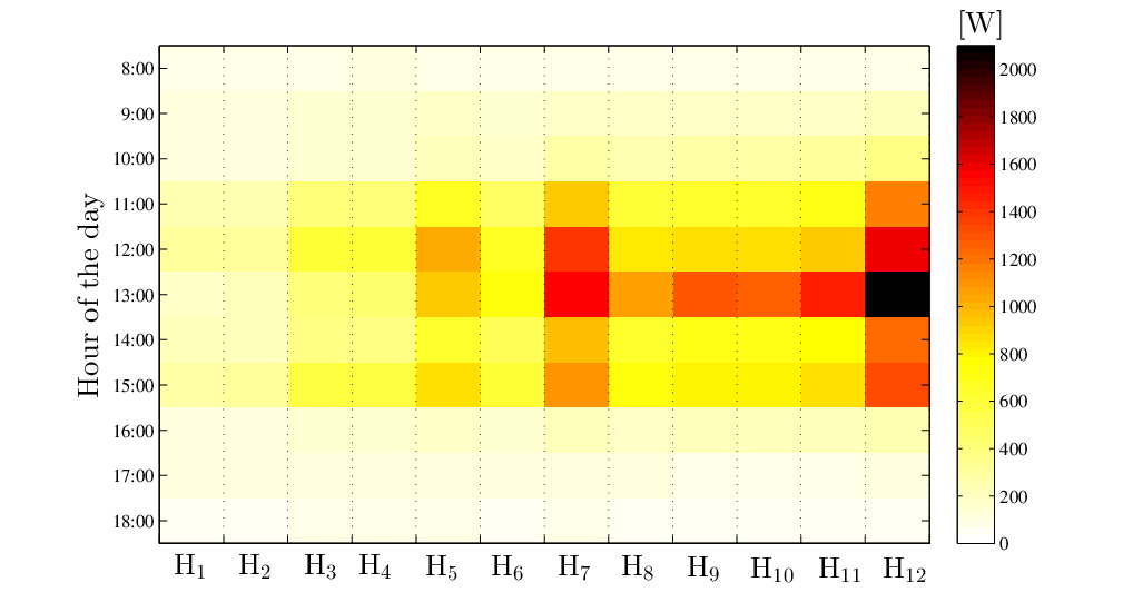
Assume that the objective of the utility company is to minimize the power losses in the network; that is, upon defining the symmetric matrix per distribution line , function is set to , with (see [11] for more details). At the customer side, function is set to . The impact of varying the parameter is investigated in detail in [11], and further illustrated in Fig. 7, where the solution of the centralized OID problem (4) is reported for different values of the parameter [cf. (3)]. Specifically, Fig. 7(a) illustrates the active power curtailed from each inverter during the course of the day when , whereas the result in Fig. 7(b) were obtained by setting . It is clearly seen that in the second case all inverters are controlled; in fact, they all curtail active power from 8:00 to 18:00. When , the OID seeks a trade off between achievable objective and number of controlled inverters. It is clearly seen that the number of participating inverters grows with increasing solar irradiation, with a maximum of inverters operating away from the business-as-usual point at 13:00.
The convergence of Algorithm 1 is showcased for , , and , and by utilizing the solar irradiation conditions at 12:00. Figure 8(a) depicts the trajectories of the iterates (dashed lines) and (solid lines) for all the houses . The results match the ones in Fig. 7(a); in fact, at convergence (i.e., for iterations ), only inverters at houses are controlled, and the active power curtailment set-points are in agreement. This result is expected, since problems (4) and (5) are equivalent; the only difference is that (4) affords only in centralized solution, whereas (5) is in a form that is suitable for the application of the ADMM to derive distributed solution schemes; see also [16, 29, 34]. Finally, the trajectories of the set-point consensus error , as a function of the ADMM iteration index are depicted in Fig. 8(b). It can be clearly seen that the algorithm converges fast to a set-point that is convenient for both utility and customers. Similar trajectories were obtained for the reactive power setpoints.
Figure 9 represents the discrepancies between local voltages on the line ; specifically, the trajectories of the voltage errors and are reported as a function of the ADMM iteration index . The results indicate that the two CEMs consent on the voltage of the branch that connects the two clusters. The “bumpy” trend is typical of the ADMM (see e.g., [29, 34]). Similar trajectories were obtained for the inverter setpoints.

VI Concluding Remarks
A suite of decentralized approaches for computing optimal real and reactive power setpoints for residential photovoltaic (PV) inverters were developed. The proposed decentralized optimal inverter dispatch strategy offers a comprehensive framework to share computational burden and optimization objectives across the distribution network, while highlighting future business models that will enable customers to actively participate in distribution-system markets.
References
- [1] E. Liu and J. Bebic, “Distribution system voltage performance analysis for high-penetration photovoltaics,” Feb. 2008, NREL Technical Monitor: B. Kroposki. Subcontract Report NREL/SR-581-42298.
- [2] E. Ntakou and M. C. Caramanis, “Price discovery in dynamic power markets with low-voltage distribution-network participants,” in IEEE PES Trans. & Distr. Conf., Chicago, IL, 2014.
- [3] K. Turitsyn, P. Súlc, S. Backhaus, and M. Chertkov, “Options for control of reactive power by distributed photovoltaic generators,” Proc. of the IEEE, vol. 99, no. 6, pp. 1063–1073, 2011.
- [4] P. Súlc, S. Backhaus, and M. Chertkov, “Optimal distributed control of reactive power via the alternating direction method of multipliers,” 2013, [Online] Available at: http://arxiv.org/pdf/1310.5748v1.pdf.
- [5] P. Jahangiri and D. C. Aliprantis, “Distributed Volt/VAr control by PV inverters,” IEEE Trans. Power Syst., vol. 28, no. 3, pp. 3429–3439, Aug. 2013.
- [6] M. Farivar, R. Neal, C. Clarke, and S. Low, “Optimal inverter VAR control in distribution systems with high PV penetration,” in IEEE PES General Meeting, San Diego, CA, Jul. 2012.
- [7] S. Bolognani and S. Zampieri, “A distributed control strategy for reactive power compensation in smart microgrids,” IEEE Trans. on Autom. Control, vol. 58, no. 11, pp. 2818–2833, 2013.
- [8] R. Tonkoski, L. A. C. Lopes, and T. H. M. El-Fouly, “Coordinated active power curtailment of grid connected PV inverters for overvoltage prevention,” IEEE Trans. on Sust. Energy, vol. 2, no. 2, pp. 139–147, Apr. 2011.
- [9] A. Samadi, R. Eriksson, L. Soder, B. G. Rawn, and J. C. Boemer, “Coordinated active power-dependent voltage regulation in distribution grids with pv systems,” IEEE Trans. on Power Del., vol. 29, no. 3, pp. 1454–1464, June 2014.
- [10] W. H. Kersting, Distribution System Modeling and Analysis. 2nd ed., Boca Raton, FL: CRC Press, 2007.
- [11] E. Dall’Anese, S. V. Dhople, and G. B. Giannakis, “Optimal dispatch of photovoltaic inverters in residential distribution systems,” IEEE Trans. Sustainable Energy, vol. 5, no. 2, pp. 487–497, Apr. 2014.
- [12] E. Dall’Anese, H. Zhu, and G. B. Giannakis, “Distributed optimal power flow for smart microgrids,” IEEE Trans. Smart Grid, vol. 4, no. 3, pp. 1464–1475, Sep. 2013.
- [13] P. Samadi, A. H. Mohsenian-Rad, R. Schober, V. Wong, and J. Jatskevich, “Optimal real-time pricing algorithm based on utility maximization for smart grid,” in Proc. of IEEE Intl. Conf. on Smart Grid Comm., Gaithersburg, MD, 2010.
- [14] N. Gatsis and G. B. Giannakis, “Residential load control: Distributed scheduling and convergence with lost AMI messages,” IEEE Trans. Smart Grid, vol. 3, no. 2, pp. 770–786, 2012.
- [15] D. P. Bertsekas and J. N. Tsitsiklis, Parallel and Distributed Computation: Numerical Methods. Englewood Cliffs, NJ: Prentice Hall, 1989.
- [16] S. Boyd, N. Parikh, E. Chu, B. Peleato, and J. Eckstein, “Distributed optimization and statistical learning via the alternating direction method of multipliers,” Foundations and Trends in Machine Learning, vol. 3, pp. 1–122, 2011.
- [17] R. Baldick, B. H. Kim, C. Chase, and Y. Luo, “A fast distributed implementation of optimal power flow,” IEEE Trans. Power Syst., vol. 14, no. 3, pp. 858–864, Aug. 1999.
- [18] F. J. Nogales, F. J. Prieto, and A. J. Conejo, “A decomposition methodology applied to the multi-area optimal power flow problem,” Ann. Oper. Res., no. 120, pp. 99–116, 2003.
- [19] G. Hug-Glanzmann and G. Andersson, “Decentralized optimal power flow control for overlapping areas in power systems,” IEEE Trans. Power Syst., vol. 24, no. 1, pp. 327–336, Feb. 2009.
- [20] T. Erseghe, “Distributed optimal power flow using ADMM,” IEEE Trans. Power Syst., 2014, to appear.
- [21] S. Magnusson, P. C. Weeraddana, and C. Fischione, “A distributed approach for the optimal power flow problem based on ADMM and sequential convex approximations,” Jan. 2014, [Online] Available at: http://arxiv.org/abs/1401.4621.
- [22] A. Y. Lam, B. Zhang, A. Domínguez-García, and D. Tse, “Optimal distributed voltage regulation in power distribution networks,” 2012, [Online] Available at http://arxiv.org/abs/1204.5226v1.
- [23] H. Zhu and G. B. Giannakis, “Multi-area state estimation using distributed SDP for nonlinear power systems,” in 3rd Int. Conf. Smart Grid Comm., Tainan City, Taiwan, Nov. 2012.
- [24] V. Kekatos and G. B. Giannakis, “Distributed robust power system state estimation,” IEEE Trans. Power Syst., vol. 28, no. 2, pp. 1617–1626, May 2013.
- [25] E. Dall’Anese and G. B. Giannakis, “Risk-constrained microgrid reconfiguration using group sparsity,” May 2014, to appear; see also: http://arxiv.org/abs/1306.1820.
- [26] A. T. Puig, A. Wiesel, G. Fleury, and A. O. Hero, “Multidimensional shrinkage-thresholding operator and group LASSO penalties,” IEEE Sig. Proc. Letters, vol. 18, no. 6, pp. 363–366, Jun. 2011.
- [27] J. Lavaei and S. H. Low, “Zero duality gap in optimal power flow problem,” IEEE Trans. Power Syst., vol. 1, no. 1, pp. 92–107, 2012.
- [28] J. Lavaei, D. Tse, and B. Zhang, “Geometry of power flows and optimization in distribution networks,” in IEEE PES General Meeting, San Diego, CA, 2012.
- [29] T. Erseghe, D. Zennaro, E. Dall’Anese, and L. Vangelista, “Fast consensus by the alternating direction multipliers method,” IEEE Trans. Sig. Proc., vol. 59, no. 11, pp. 5523–5537, 2011.
- [30] L. Vandenberghe and S. Boyd, “Semidefinite programming,” SIAM Review, vol. 38, no. 1, pp. 49–95, Mar. 1996.
- [31] R. Grone, C. R. Johnson, E. M. Sá, and H. Wolkowicz, “Positive definite completions of partial Hermitian matrices,” Linear Algebra and its Applications, vol. 58, pp. 109–124, 1984.
- [32] R. A. Jabr, “Exploiting sparsity in SDP relaxations of the OPF problem,” IEEE Trans. Power Syst., vol. 2, no. 27, pp. 1138–1139, May 2012.
- [33] M. Braun, J. Künschner, T. Stetz, and B. Engel, “Cost optimal sizing of photovoltaic inverters – influence of of new grid codes and cost reductions,” in Proc. of 25th Europ. PV Solar Energy Conf. and Exhib., Valencia, Spain, Sep. 2010.
- [34] H. Zhu, G. B. Giannakis, and A. Cano, “Distributed in-network channel decoding,” IEEE Trans. Sig. Proc., vol. 57, no. 10, pp. 3970–3983, 2009.