Analysis of single pulse radio flux measurements of PSR B1133+16 at 4.85 and 8.35 GHz
Abstract
We show the results of microsecond resolution radio data analysis focused on flux measurements of single pulses of PSR B1133+16. The data were recorded at 4.85 GHz and 8.35 GHz with 0.5 GHz and 1.1 GHz bandwidth, respectively, using Radio Telescope Effelsberg (MPIfR). The most important conclusion of the analysis is, that the strongest single pulse emission at 4.85 GHz and 8.35 GHz contributes almost exclusively to the trailing part of the leading component of the pulsar mean profile, whereas studies at lower frequencies report that the contribution is spread almost uniformly covering all phases of the pulsar mean profile. We also estimate the radio emission heights to be around 1%–2% of the light cylinder radius which is in agreement with previous studies. Additionally these observations allowed us to add two more measurements of the flux density to the PSR B1133+16 broadband radio spectrum covering frequencies from 16.7 MHz up to 32 GHz. We fit two different models to the spectrum: the broken power law and the spectrum based on flicker noise model, which represents the spectrum in a simpler but similarly accurate way.
Keywords:
pulsars: general – pulsars: individual: B1133+161 Introduction
Pulsar radio emission is still not explained in details but it is believed to originate close to the pulsar surface (Krzeszowski et al. 2009 and references therein). The analysis of 62 mean profiles of 23 pulsars at different frequencies regarding aberration and retardation effects yielded the estimation of the emission height being below 1500 km, but most probably being of the order of 500 km above the pulsar surface. The advance in theoretical understanding of the emission mechanism and conditions in the magnetosphere have been driven mainly by the observations. Recently many observations have been concentrated on observing single pulses which carry detailed information about the physics of radio emission. Analysis of single pulse high resolution time series can show a few interesting properties i.e. giant and bright pulses, subpulse drift, nulling, microstructure, etc. Observations of single pulses for most pulsars may be carried out mainly at lower frequencies because pulsars are weak radio sources at high frequencies which is clearly seen in their steep spectra. The pulsar spectrum in general can be described by a power law , where is the spectral index. The average spectral index for 266 pulsars for frequency spread from 0.4 to 23 GHz is (Maron et al., 2000).
| BNAME | B1133+16 |
|---|---|
| JNAME | J1136+1551 |
| 1.188 s | |
| s s-1 | |
| RA (J2000) | 11h36m03s |
| DEC (J2000) | 15∘51’04” |
| DM | 4.86 pc cm-3 |
| RM | 1.1 rad m2 |
| Age | Yr |
| Distance | 350 20 pc |
| Proper motion | 375 mas yr-1 |
| Transverse velocity | km s-1 |
| G | |
PSR B1133+16 is a nearby middle–aged pulsar with one of the highest proper motion, and thus, one with the highest transverse velocity (Brisken et al., 2002). Basic properties of PSR B1133+16 are gathered in Table 1. Its faint optical counterpart (B=28.1 0.3 mag) was firstly detected by Zharikov et al. (2008). Recently Zharikov & Mignani (2013) detected the optical candidate of the pulsar counterpart on the GTC and VLT images that is consistent with the radio coordinates corrected for its proper motion. This source was also detected in X-rays by Kargaltsev et al. (2006) using the Chandra satellite with the flux of (0.8 0.2) ergs cm-2 s-1 in the 0.5–8.0 keV range. For the X–rays fit the assumed hydrogen column density was cm-2. Low value of and no Balmer bow shock imply a low density of ambient matter around the pulsar. This pulsar has not been detected by the Fermi satellite.
In this paper in Sec. 2 we describe observational parameters and technical issues about the recorded data. Sec. 3 covers analysis of the data. We present two different approaches for data analysis: mean profiles composed of pulses that their flux fall into specific intensity range as well as the phase position and flux of single pulses that are stronger than 20. In Sec. 4 we discuss radio emission height estimations, while in Sec. 5 we present the radio spectrum of PSR B1133+16 and discuss different spectrum models. We conclude our results in Sec. 6.
2 Observations and data reduction
Our analysis is based on the Radio Telescope Effelsberg archival data. The observational settings and parameters are collected in Table 2. Observations were made using the 4.85 GHz and the 8.35 GHz receivers of the MPIfR 100 m radio telescope in Effelsberg. The receivers have circularly polarised feeds. Both receivers feature cryogenically cooled High-Electron-Mobility Transistor (HEMT) low noise input stages with typical system temperatures of 27 K for the 4.85 GHz receiver and 22 K for the 8.35 GHz receivers. A calibration signal can be injected synchronously to the pulse period for accurate measurements of pulsar flux densities. The Effelsberg radio telescope is regularly calibrated on catalogued continuum sources and we used the mean height of the injected calibration signal of 1.2 K for 4.85 GHz and 2.083 K for 8.35 GHz for the flux calibrations. The two intermediate frequency (IF) signals (bandwidths of 500 MHz for 4.85 GHz and 1.1 GHz for 8.35 GHz) from each receiver, one for left hand (LHC) and one for right hand (RHC) circular polarisation are detected in a broad–band polarimeter attached to the receiver, providing four output independent signals relating to the power levels of LHC, RHC, LHCRHCLHC,RHC, LHCRHCLHC,RHC. No dedispersion was used before or after the detection due to low value of DM of PSR B1133+16. The dispersion broadening amounts to 178 s and 78 s for 4.85 GHz and 8.35 GHz, respectively, which is of the order of their sampling rates. The four detected power levels are linearly encoded as short pulses of a variable frequency of typically 2–3 MHz corresponding to the system noise level, but ranging up to a maximum of 10 MHz. These signals were brought down to the station building and using the EPOS backend, the four frequency encoded power levels were recorded synchronously to the pulse period in 1024 phase bins (=samples) per period. The average signal power for each phase bin was determined by simply counting the number of pulses of the supplied frequency encoded signal for the duration of the phase bin and then recording the counts on disk for later off-line processing. Only the data from LHC and RHC channels were used and added together to yield the detected total power for our analysis. The individual phase bins had durations of 200 s for 4.85 GHz and 60 s for 8.35 GHz. With the given system temperatures and the respective antenna efficiencies of 1.5 K/Jy and 1.2 K/Jy, we achieved a typical sensitivity (rms) of 30 mJy and 80 mJy per single pulse phase bin for the two frequencies, respectively.
2.1 Digitisation effects
The aforementioned sensitivity corresponds to a fraction of of the equivalent background (baseline) noise level of 16–18 Jy. At the same time, we recorded typically only 600 (4.85 GHz) down to 200 (at 8.35 GHz) frequency encoded counts per phase bin. As a result, one finds that the signal power is resolved in steps of 30 mJy and 80 mJy for the two receivers and that the rms noise fluctuations are barely resolved, amounting to a couple of counts at most (see Fig. 1).
2.2 Weather and radio interference
Weather, especially clouds, changes the opacity of the atmosphere and as a consequence we found that fluctuations of the sky background were of the order of a fraction of a Kelvin on the short timescales (200 ms and 60 ms) that were used for the measurement window and the subtraction of the noise baseline. Both receivers were also affected by a very low level 100 Hz modulation ( of the baseline level) originating in the receiver’s power supply and cooling systems. With typical observed pulse component widths of 5–10 ms, we find that we cannot rule out that weak individual components of individual single pulse may be affected by the interference. However, averaging and other statistical flux estimates using sufficient numbers (10) of single pulses would not be affected by weather induced noise fluctuations or power supply interference.
The above mentioned effects are visible in the data as approximately linear trends added to each of the recorded single pulses. One example of such slope and effects of the correction at 8.35 GHz is presented in Fig. 1. The values of the slopes show no trends from pulse to pulse and they range from -2 to 2 mJy / bin and their distribution is a Gaussian–like with a zero mean. The behaviour of the system at 4.85 GHz is roughly the same as of 8.35 GHz data and the same correction routines were applied.
| Date | 2002 Feb 07 | 2004 Apr 26 |
|---|---|---|
| Frequency | 4.85 GHz | 8.35 GHz |
| Bandwidth | 0.5 GHz | 1.1 GHz |
| Observing time | 67 min. | 120 min. |
| Number of pulses | 3361 | 6029 |
| Sampling time | 200 s | 60 s |
| Mean flux density | 1.59 mJy | 0.73 mJy |

3 Single pulses in microsecond resolution
Average profiles of PSR B1133+16 at 4.85 GHz and 8.35 GHz consist of two main components connected by a bridge of emission (Fig. 2). The leading component is approximately five times stronger than the trailing one and they are separated by around 5∘. The duty cycle of this pulsar is around 3% at 4.85 GHz and 8.35 GHz.

We performed an analysis of microsecond resolution radio data focused on flux measurements of single pulses. High resolution observations allowed us to investigate the microstructure of single pulse shapes. The single pulse at 8.35 GHz in the top panel of Fig. 3 shows interesting features in the trailing component. On the other hand the bottom panel of Fig. 3 is focused on the leading component of another single pulse profile at the same frequency. As it can be clearly seen, single pulse profiles have complex structures, which can be resolved only with high time resolution observations. There were numerous studies of the microstructure of PSR B1133+16 and other pulsars (e.g. Ferguson & Seiradakis 1978; Lange et al. 1998). It is reported that microstructure is most probably related to the emission process and is present in many pulsars with the fraction of pulses showing microstructure being of the order of 30% to 70% (Lange et al., 1998).


3.1 Timescale constraints on geometrical parameters
The timescale of real-time flux variability (such as the micro- or nano–structure) can be interpreted in terms of the size of the emitting region, or in terms of the angular size of relativistically–beamed radiation pattern (Lange et al. 1998, Crossley et al. 2010). The outcome depends on the actual spatial and temporal structure of the emission region, and its relation to the angular scale of the radiated beam.
Let us consider a localised, and relativistically-outflowing source of radio emission, e.g. a cloud of charges with Lorentz factor moving along a narrow bunch of magnetic field lines. Here narrow means that the spread of -field direction within the emitting stream, as measured for different rotational azimuths, is smaller than the intrinsic size of the emission pattern . In the observer’s reference frame the charges move along a narrow bunch of trajectories with the radius of curvature . If the source emits detectable radiation for a limited period of time (as measured in our reference frame) an observed spike of radio flux has a width of (since the outflowing source is nearly catching up with the emitted photons). If the source persists for a time sufficient to sweep its full beam across the observer’s line of sight, then , and the timescale is:
| (1) |
where cm and (Jackson, 1975). During that time the point source moves up in pulsar magnetosphere by a distance of . For cm the observed timescale of the microstructure of s limits the Lorentz factor to the mildly relativistic value . For the observed timescale implies cm, comparable to the light cylinder radius of PSR B113316 ( cm). Note that for the curvature radiation from a localised emitter, by definition one expects , where is the observed frequency (a few GHz). That is, the pair of values and must ensure that the curvature spectrum extends up to the frequency . The observed time scale of the microstructure ( s) is then too long to directly correspond to the rapid sweep of the elementary beam of the curvature radiation emitted by a small plasma cloud.
Another case is encountered when the emitting clouds extend considerably along -field lines (), or when there is a steady outflow of uniformly-distributed matter that emits radio waves. Again, let us first consider the narrow stream case, in which the internal spread of rotational azimuths of is much smaller than the size of the relativistic beam (). In such a case, projection of the beam on the sky results in an elongated stripe of width . The observed timescale is then determined by the speed of sightline passage through the stripe, as resulting from the rotation of the neutron star:
| (2) | |||
where is the viewing angle between the sightline and the rotation axis, and is the ‘cut angle’ between the sky-projected emission stripe and the path of the line of sight while it is traversing through the beam (see Fig. 2 in Dyks & Rudak 2012). Lange et al. (1998) provide a similar timescale estimate (eq. 6 therein) which is valid only for , i.e. for orthogonal passage of the sightline through the beam. For the parameters and determined by Gangadhara et al. (1999), the observed separation of components () implies . Eq. (2) then gives , which is smaller than the minimum Lorentz factor required for the curvature spectrum to extend up to the observed frequency of a few GeV.
In a thick stream case, the spread of rotational azimuths of within the stream is much larger than the angular size of the stream (). The emitted radiation can be considered (approximately) tangent to the local magnetic field, and to the charge trajectory in the observer’s frame. The observed timescale is then determined by the angular extent of the stream in the magnetic azimuth , measured around the dipole axis. For the stream extending between and the timescale is equal to , where the pulse longitudes and correspond to the moments when our sightline starts and stops probing the region of the stream. For known (or assumed) , , and the values of and can be calculated from eqs. (18) and (19) in (Dyks et al., 2010). However, the timescale of s corresponds to the angle which requires . Thus, for PSR B113316 the thick stream case may need to be considered only for a few thousands.
3.2 Single pulse flux distribution
We define bright pulses as those with energy of ten times greater than the mean flux of the pulsar. Looking closer at the flux density distribution (Fig. 4) one can see that there are not many bright pulses in our time series, only around 0.9% at both frequencies.


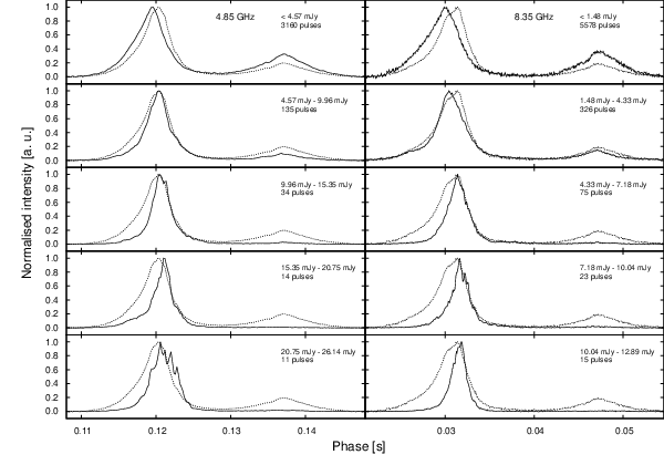
All flux measurements (Fig. 4) for both frequencies were divided into ten equally sized intensity ranges (Nowakowski, 1996). The ranges were constructed as follows: the minimum and maximum flux measurements from each data set were taken as boundaries and all remaining pulse flux values were assigned to one of the () / 10 ranges of the widths of around 5 mJy and 3 mJy for 4.85 GHz and 8.35 GHz, respectively. The minimum and maximum flux values are 0.83 mJy and 53.11 mJy as well as 1.38 mJy and 27.15 mJy for 4.85 GHz and 8.35 GHz data, respectively. Negative flux values are introduced into the data because of observing system properties which were discussed in detail in Sec. 2 and stochastic noise properties in pulses with no detection. For the single pulses with flux falling into a particular range the average profiles were constructed. Normalised profiles for 4.85 GHz and 8.35 GHz data and respective mean profiles of first five intensity ranges are presented in Fig. 5. The number of pulses falling into specific intensity range is written in each panel and also shown in the Fig. 4 above the distributions. In the Fig. 5 it is easily noticeable that the maximum of the intensity level averaged profile (solid line) moves towards later phases with respect to the maximum of the mean pulsar profile (dotted line) for both frequencies and the shift is increasing with frequency from 0.36∘ at 4.85 GHz to 0.55∘ at 8.35 GHz. It means that low intensity single pulses contribute mainly to the leading part of first component, whereas higher intensity single pulses contribute almost exclusively to its trailing part. On the other hand the second component is composed mainly of the lowest intensity single pulses — it is visible only in the first two intensity ranges. The shifts of pulsar components were also investigated by Mitra et al. (2007). They report that the stronger emission of B0329+54 comes earlier than the weaker emission with a delay of 1.5∘. This is opposite to what we have observed. Moreover, Mitra et al. investigated the effect only at one frequency, i.e. 325 MHz. Therefore, further investigations of more pulsars single pulses are highly recommended because the mechanism behind observed effect is not understood and one does not know how common it may be in other pulsars.
It is clearly visible in Fig. 6 that at 4.85 GHz and 8.35 GHz maximum flux values (denoted with dots) contribute almost only to the trailing edge of the first component of the mean profile, whereas studies at lower frequencies report that the contribution is spread almost uniformly covering all phases of the pulse mean profile (Karuppusamy et al., 2011). A mean profile composed only of single pulses with SNR is plotted with a solid line, whereas the mean profile composed of all of the single pulses is plotted with a dotted line. The numbers of such pulses are 758 (23%) at 4.85 GHz and 407 (7%) at 8.35 GHz, respectively.

4 Emission heights
In the case of 8.35 GHz data from Fig. 5 (right hand side panels) one can read out the shift of 0.0018 seconds ( 0.55∘ = 0.001 rad) between the longitude of the low-flux and high-flux emission. Ignoring (for a while) the curved shape of B-field lines, this shift can be translated to altitude difference: cm (independent of and ). However, the radius of curvature of B–field lines at the rim of polar cap of this pulsar is cm. The upward shift of emission by , results then in a change of emission direction by 0.27 rad 15∘, which is much larger than the observed displacement of 0.5∘. Therefore, if the observed misalignment of low–flux and high–flux emission has anything to do with the real spatial shift of emission region, it must be dominated by the effect of curved B–field lines rather than the aberration–retardation shift. Unfortunately, in such a case a full information on geometry is needed to determine or . The same logic applied to 4.85 GHz data (left hand side panels Fig. 5) yields the following results: rad, cm and which is also much bigger than the measured shift of 0.36∘.
Using and (Gangadhara et al., 1999) and canonical formulae (Lorimer, 2005) we derived radio emission heights at 4.85 GHz and 8.35 GHz. While making the height estimates we associate the peak separation with two different sets of B–field lines: the last open field lines which have the standard magnetic colatitude , and with the critical field lines, which have .
Simple calculations yield the estimations of emission heights at 4.85 GHz are 67cm and 122cm for the last open and critical magnetic field lines, respectively, whereas for stronger emission it is closer to the neutron star surface at 66cm and 120cm. Similarly, at 8.35 GHz, emission heights are 66cm and 122cm for the last open and critical field lines, respectively, whereas for stronger emission it is 65cm and 119cm. Our analysis shows that the emission region is located at a distance of around 1%-2% of the light cylinder radius from the pulsar surface which is consistent with earlier studies (e.g. Krzeszowski et al. 2009).
5 Radio spectrum
In general pulsars have steep spectra with an average spectral index around (Maron et al., 2000). Except for basic spectrum (that can be described with power law ) there are two common types: spectrum with a break (described with two power laws) and spectrum with a turn–over (clearly visible maximum flux). We collected flux density measurements from different publications (Table 3). Our dataset covers a very wide radio frequency range from 16.7 MHz up to 32 GHz. The analysis of the data presented in this paper yielded the mean flux values of 1.59 mJy and 0.73 mJy at 4.85 GHz and 8.35 GHz, respectively, with an estimated error of 10% of the original value. The spectrum of PSR B1133+16 spanning the wide radio frequency range is shown in Fig. 7. Each point denotes a measurement of mean flux density with respective uncertainties. We included the measurements by Karuppusamy et al. (2011) at 7 frequencies, ranging from 116.75 MHz to 173.75 MHz. The authors claim that the spectrum of PSR B1133+16 over their ”reasonably wide frequency range” of 57 MHz is of a broken power law type with spectral indices of and . In Fig. 7 we have indicated their spectrum by a dashed line. We cannot confirm Karuppusamy’s spectral indices which were obtained from low frequency measurements covering only a small range of frequencies. However, we find that Karuppusamy’s measurements have a typical spread of flux values and thereby fit well into the overall spectrum as can be seen in Fig. 7.

Our spectrum of PSR B1133+16 may be described by two power laws in the whole frequency range with and with a break frequency of MHz ().
To reproduce the spectrum of PSR B1133+16 covering over 32 GHz frequency range we have also fitted the flicker noise model proposed by Löhmer et al. (2008) which is described by
| (3) |
where S0 is a scaling factor, , is an observing frequency, is a characteristic time for the nano–burst decay time, and n is the exponent which constrains a combination of physical parameters of nano pulses (for details refer to Löhmer et al. 2008). Our fitted parameters of , and are in good agreement with Löhmer et al. (2008) result and our reduced is comparable to the value for the broken power law fit. The model, apart from the scaling factor S0, is based on only two physical parameters. The first one is the duration of a nano–pulse () and the second one (n) is related to the geometry of the emission process. It is based on the assumption that the pulsar radio emission is in fact the superposition of many nano–pulses, which in case of PSR B1133+16 have duration of ns according to Löhmer et al. (2008). However our fit gives even shorter nano–pulse duration of 0.4 ns. Löhmer et al. (2008) report that for 12 pulsars 0.1 ns 2.0 ns.
| Frequency | Flux | Error | Reference | Frequency | Flux | Error | Reference |
|---|---|---|---|---|---|---|---|
| [MHz] | [mJy] | [mJy] | [MHz] | [mJy] | [mJy] | ||
| 16.7 | 310 | 50 | [1] | 156 | 580 | 58 | [1] |
| 16.7 | 1410 | 320 | [1] | 160 | 520 | 80 | [1] |
| 20 | 700 | 100 | [1] | 170 | 380 | 150 | [1] |
| 25 | 560 | 100 | [1] | 173.75 | 380 | 38 | [4] |
| 25 | 1900 | 230 | [1] | 196 | 560 | 260 | [1] |
| 34.5 | 900 | 90 | [1] | 270 | 790 | 190 | [1] |
| 39 | 740 | 107 | [1] | 275 | 475 | 85 | [1] |
| 39 | 620 | 90 | [2] | 341 | 320 | 60 | [5] |
| 53 | 1105 | 260 | [1] | 370 | 305 | 124 | [1] |
| 61 | 830 | 170 | [1] | 408 | 256 | 53 | [6] |
| 61 | 700 | 140 | [2] | 606 | 144 | 35 | [6] |
| 74 | 780 | 150 | [1] | 626 | 120 | 40 | [5] |
| 80 | 640 | 70 | [1] | 925 | 37 | 11 | [6] |
| 80 | 1000 | 500 | [1] | 1400 | 24.92 | 15.33 | [7] |
| 85 | 910 | 150 | [1] | 1408 | 32 | 5 | [6] |
| 85 | 770 | 130 | [2] | 1412 | 60 | 20 | [5] |
| 100 | 420 | 150 | [1] | 1606 | 51 | 15 | [6] |
| 102 | 1210 | 180 | [1] | 2300 | 7.07 | 3.24 | [7] |
| 102 | 1280 | 550 | [3] | 2700 | 8.7 | 0.6 | [7] |
| 102 | 1520 | 660 | [1] | 4850 | 2.7 | 1.07 | [7] |
| 102 | 1020 | 200 | [2] | 4850 | 2.4 | 0.5 | [5] |
| 111 | 770 | 190 | [1] | 4850 | 1.59 | 0.16 | this paper |
| 116.75 | 550 | 55 | [4] | 8350 | 0.73 | 0.07 | this paper |
| 130 | 720 | 72 | [4] | 8500 | 0.86 | 0.12 | [7] |
| 139.75 | 1000 | 100 | [4] | 10550 | 0.63 | 0.12 | [7] |
| 142.25 | 1000 | 100 | [4] | 14600 | 0.169 | 0.0507 | [7] |
| 147.5 | 580 | 58 | [4] | 14800 | 0.26 | 0.078 | [7] |
| 151 | 1100 | 170 | [1] | 24000 | 0.178 | 0.0534 | [7] |
| 151 | 805 | 75 | [1] | 32000 | 0.03 | 0.02 | [7] |
| 156 | 800 | 80 | [4] | 32000 | 0.055 | 0.06 | [8] |
6 Conclusions
The analysis of PSR B1133+16 single pulses is a process that needs a certain amount of care. First off all, it is important to take into account different observational and technical effects that can affect recorded data, especially with very high time resolution. The effects that are presented in this paper play huge role and alter the data significantly. Understanding of such effects and their influence on the data recording process is important for proper data reduction. Some of the effects are not visible in the mean profiles but only in single pulses data.
The mean profiles of PSR B1133+16 at 4.85 GHz and 8.35 GHz consist of two components (Fig. 2). The second component is emitted almost exclusively by low intensity individual pulses. On the other hand, the first component is seen in single pulses regardless of their intensity except for the cases when it is not present at all. However, lower intensity emission contributes mostly to the leading part of the first component whereas higher intensity single pulses contribute mainly to its trailing part (Fig. 5) which was also reported by Maron et al. (2013). The results of analysis of 4.85 GHz and 8.35 GHz data are consistent with previous studies by (Nowakowski, 1996) at 430 MHz but studies of B0329+54 (Mitra et al., 2007) show entirely opposite behaviour without full explanation. This inconsistency requires further studies of other pulsars single pulses to explain this effect.
We show, in contradiction to studies at lower frequencies by Karuppusamy et al. (2011), who report an almost uniform spread of single pulse maxima, that the maximum emission of B1133+16 single pulses at 4.85 and 8.35 GHz contributes almost exclusively to the trailing part of the leading component of the mean profile. Our result is consistent with the behaviour at 341, 626, 1412 and 4850 HMz mentioned by Kramer et al. (2003) and extends the studies up to 8.35 GHz.
Radio emission arises close to the pulsar surface at the distances of around 65 stellar radii at frequencies of 4.85 GHz and 8.35 GHz. Weaker emission, which contributes to the leading part of the leading components, comes in earlier phases which suggests that originates in magnetosphere further from the pulsar surface than more energetic emission. Our calculations shows, that the difference of the emission heights for stronger and weaker emission is of the order of a few stellar radii, amounting to a change of 1%–2% of the emission height, which is consistent with previous estimations (Krzeszowski et al., 2009).
There are 60 mean flux measurements in the literature of PSR B1133+16 that are known to us. They span a very wide radio frequency range from 16.7 MHz up to 32 GHz. To reproduce the spectrum we fitted two different models: the broken power–law model and one based on flicker noise model of pulsar radio emission (Löhmer et al., 2008). Surprisingly, the model proposed by Löhmer et al. (2008) is not widely used in the literature although it reproduces the pulsar spectrum comparably well to the power-law model. Future high time resolution observations might be useful to verify nano–pulse emission model.
Due to the fact, that the pulsar radio emission is weaker at higher frequencies, giant pulses are the ones that can allow us to study closely their structure. In our both data samples there is roughly one per cent of bright pulses that are at least ten times stronger than mean flux and their microstructure is clearly visible.
Acknowledgements
The presented results are based on the observations with the 100–m telescope of the MPIfR (Max-Planck-Institut für Radioastronomie) at Effelsberg. This work has been supported by Polish National Science Centre grants DEC-2011/03/D/ST9/00656 (KK, AS), DEC-2012/05/B/ST9/03924 (OM) and DEC-2011/02/A/ST9/00256 (JD). Data analysis and figures were partly prepared using R (R Core Team, 2013).
References
- Brisken et al. (2002) Brisken W. F., Benson J. M., Goss W. M., Thorsett S. E., 2002, ApJ, 571
- Crossley et al. (2010) Crossley J. H., Eilek J. A., Hankins T. H., Kern J. S., 2010, ApJ, 722
- Dyks & Rudak (2012) Dyks J., Rudak B., 2012, MNRAS, 420
- Dyks et al. (2010) Dyks J., Rudak B., Demorest P., 2010, MNRAS, 401
- Ferguson & Seiradakis (1978) Ferguson D. C., Seiradakis J. H., 1978, A&A, 64
- Gangadhara et al. (1999) Gangadhara R. T., Xilouris K. M., von Hoensbroech A., Kramer M., Jessner A., Wielebinski R., 1999, A&A, 342
- Izvekova et al. (1981) Izvekova V. A., Kuzmin A. D., Malofeev V. M., Shitov I. P., 1981, A&AS, 78
- Jackson (1975) Jackson J. D., 1975, Classical electrodynamics. Wiley
- Kargaltsev et al. (2006) Kargaltsev O., Pavlov G. G., Garmire G. P., 2006, ApJ, 636
- Karuppusamy et al. (2011) Karuppusamy R., Stappers B. W., Serylak M., 2011, A&A, 525
- Kramer et al. (2003) Kramer M., Karastergiou A., Gupta Y., Johnston S., Bhat N. D. R., Lyne A. G., 2003, A&A, 407
- Krzeszowski et al. (2009) Krzeszowski K., Mitra D., Gupta Y., Kijak J., Gil J., Acharyya A., 2009, MNRAS, 393
- Lange et al. (1998) Lange C., Kramer M., Wielebinski R., Jessner A., 1998, A&A, 332
- Löhmer et al. (2008) Löhmer O., Jessner A., Kramer M., Wielebinski R., Maron O., 2008, A&A, 480
- Lorimer (2005) Lorimer D., 2005, Handbook of Pulsar Astronomy. Cambridge Observing Handbooks for Research Astronomers, Cambridge University Press
- Lorimer et al. (1995) Lorimer D. R., Yates J. A., Lyne A. G., Gould D. M., 1995, MNRAS, 273
- Malofeev (1999) Malofeev V. M., 1999, Katalog radiospektrov pul’sarov, Pushchino:PRAO
- Malofeev et al. (2000) Malofeev V. M., Malov O. I., Shchegoleva N. V., 2000, Astronomy Reports, 44
- Manchester et al. (2005) Manchester R. N., Hobbs G. B., Teoh A., Hobbs M., 2005, AJ, 129
- Maron et al. (2000) Maron O., Kijak J., Kramer M., Wielebinski R., 2000, A&AS, 147
- Maron et al. (2013) Maron O., Serylak M., Kijak J., Krzeszowski K., Mitra D., Jessner A., 2013, A&A, 555
- Mitra et al. (2007) Mitra D., Rankin J. M., Gupta Y., 2007, MNRAS, 379
- Nowakowski (1996) Nowakowski L. A., 1996, ApJ, 457
- R Core Team (2013) R Core Team 2013, R: A Language and Environment for Statistical Computing. R Foundation for Statistical Computing, Vienna, Austria
- Zharikov & Mignani (2013) Zharikov S., Mignani R. P., 2013, MNRAS, 435
- Zharikov et al. (2008) Zharikov S. V., Shibanov Y. A., Mennickent R. E., Komarova V. N., 2008, A&A, 479