Generic nonequilibrium steady states in asymmetric exclusion processes on a ring with bottlenecks
Abstract
Generic inhomogeneous steady states in an asymmetric exclusion process on a ring with a pair of point bottlenecks are studied. We show that due to an underlying universal feature not considered hitherto, measurements of coarse-grained steady state densities in this model resolve the bottleneck structures only partially. Unexpectedly, it displays localization-delocalization transitions, and confinement of delocalized domain walls, controlled by the interplay between particle number conservation and bottleneck competition for moderate particle densities.
I Introduction
Simplest physical modeling of classical transports in low dimensions are often made in terms of asymmetric exclusion processes. For instance, one-dimensional (1D) totally asymmetric simple exclusion process (TASEP) with open boundaries provides a simple physical description of restricted 1D motion in various natural [1] and social phenomena [2]; see Refs. [3, 4] for basic reviews on asymmetric exclusion processes. In this article we investigate the generic relationship between the inhomogeneous steady state densities, and conservation laws and structural deformations in asymmetric exclusion processes with periodic boundary conditions. To this end, we study the generic inhomogeneous steady states in a 1D model that executes TASEP on a ring having a pair of bottlenecks. We show that bottleneck competitions in the model leads to screening or irrelevance of one bottleneck by the other for moderate densities. Significantly, this implies that coarse-grained measurements of the inhomogeneous densities in closed TASEP cannot be reliably used to obtain information about the underlying microscopic bottlenecks, as experiments detect them only partially, establishing an underlying universal feature distinctly different from critical phenomena or critical dynamics. Furthermore, for moderate densities depending upon the strengths of the bottlenecks, our model displays both localized (LDW) and delocalized (DDW) domain walls, in contrast to open TASEPs [5]. Unexpectedly, DDWs can be smoothly confined by tuning the relative positions of the bottlenecks. Our results have experimental implications, e.g., in studies of unidirectional circular ribosome translocations along messenger RNA (mRNA) loops with defects or slow codons in cells [6, 7].Our model should serve as an important step for theoretical analysis of the mutual interplay between particle number conservation and arbitrary number of discrete bottlenecks in asymmetric exclusion processes in 1D closed systems. The rest of the paper is organized as follows: In Sec. II, we construct our model. Then in Secs. III.1 and III.2, we elucidate the different inhomogeneous and homogeneous density phases of the system. Finally, we summarize in Sec. V.
II Construction of our model
Our 1D model consists of a ring having sites, with two bottlenecks (point defects) of reduced hopping rates , from to and to , respectively. Hopping rates elsewhere is unity; see Fig. (1). Site labels run clockwise from , whereas particles move anticlockwise. When one of is set to unity, our model is physically identical to that of Ref. [8]. It is convenient to use a continuum labeling in thermodynamic limit (TL): , . The bottleneck positions are then at and . With number of particles in the system, we define a mean density . The nonequilibrium steady states in our model and the associated phase transitions are parametrized by .

It is useful here to compare our model with the existing literature on TASEP with disorder. For instance Refs. [9, 10], discuss the effects of multiple defects in an open TASEP channel (see also Ref.[11] for general discussions on inhomogeneous TASEPs). In the model of Ref. [9] one or two point defects have been considered. Their effects on the steady state current has been obtained. This has been generalized in Ref. [10], where instead of point defects, extended defects of variable sizes are discussed. Subsequently, Ref. [12] has studied the TASEP with site-wise disorder and has obtained a set of exact results in the low current regime. In contrast to the models in Refs. [9, 10, 11, 12], our model is a closed model having no edge or boundary effects, and thus with no entry or exit of particles. Evidently, the dynamics keeps the particle number in our model strictly conserved. Conservation laws are known to affect the universal scaling properties of fluctuations in equilibrium or nonequilibrium systems [13, 14]. How conservation laws affect the ensuing (possibly nonuniform) steady states in inhomogeneous nonequilibrium systems remains a theoretically interesting question. Our model is ideally suited to study this issue. In particular, the two defect sites in our model in general have unequal hopping rates (), unlike the models in Refs. [9, 10], where the bottlenecks are considered to have equal hopping rates.
III Steady state density profiles
On general ground, the system should be in three different phases: (i) Low Density (LD) [High density (HD)], with the lattice being nearly empty [full] and consequently the bottlenecks affecting the density profile only locally in the form of a boundary layer (BL) of vanishing thickness in TL behind the bottleneck, and (ii) Intermediate Density (ID), with between LD and HD phases, when there are macroscopic effects of the defects on the density profile in the form of generic LDWs and their delocalization transitions. Notice that the dynamics of TASEP is formally given by rate equations for every site, that involves nonlinear coupling with neighboring sites, and hence not closed [11]. In our work below, we use analytical mean-field theory (MFT), complemented by our extensive Monte-Carlo Simulations (MCS) (with random sequential updates), for quantitative descriptions of these steady-states. In MFT descriptions, one proceeds by neglecting spatial correlations and replacing products of averages by averages of products. We begin with the analysis for the nontrivial ID phase below, followed by the LD and HD phases.
III.1 Intermediate density phase
We study inhomogeneous steady states for moderate densities (Intermediate density (ID) phase) by using analytical mean-field theory (MFT), developed by exploiting the spatial constancy of the steady-state currents, complemented by extensive Monte-Carlo Simulations (MCS) (with random sequential updates). The steady state density follows
| (1) |
neglecting terms which are insignificant in the bulk in TL (strictly, Eq. (1) holds away from the BLs, which may form close to a defect). Thus, in the bulk, should be a constant [15]. Therefore, in ID phase, can be piecewise continuous without any spatial variation, with the possibility of an LDW in the system. The system can be viewed as a combination of two TASEP channels , marked as a blue dashed-dotted line in Fig. 1, and (black dashed line in Fig. 1), joined at and respectively [16]; see Fig. 1. Channels and are generally of unequal length. Define with as densities for . Thus, in terms of and , locations of and are given by and , respectively. We establish below the conditions on for ID phase. If for both , ID phase holds (see below), there should be an LDW for each of them. Since the LDW height depends on the hopping rates at the bottleneck, the two putative LDWs due to impose different steady state currents in different bulk regions of the system, which is unphysical. Assuming the principle of minimum current [17], that imposes the minimum current in the system creates an LDW behind it; the other bottleneck creates only a boundary layer (BL) with a vanishing thickness in TL, being rendered subdominant or irrelevant in TL (see Fig. 2).
For concreteness, now consider and an LDW in at ; has a uniform density in the bulk. Assume ( may be analyzed by the particle-hole symmetry). Then,
| (2) |
In addition, at , has a BL of value . Current conservation at leads to yielding
| (3) |
Further, current conservation in yields and since ,
| (4) |
For a BL of height and vanishing thickness in TL at , current conservation leads to
| (5) |
From current conservation at , . Further, particle number conservation (PNC)
| (6) |
yields (see Fig. 2)
| (7) |
as the LDW position in . Equation (7) appears to yield a diverging as . However, in that limit with , the model is no longer in the ID phase and Eq. (7) does not apply. As expected, depends only on [18]. Notice that ; thus an LDW is just formed at the location of . Hence, this yields , or , setting the boundary between the ID and Low Density (LD) phase. Particle-hole symmetry immediately yields , or, as the boundary between the ID and High Density (HD) phases. Thus, for , ID phase ensues. If for some , both satisfy ID phase conditions, then there is an LDW due only to ; the putative LDW due to , that would have existed with and , gets suppressed to a BL with a vanishing thickness in TL. Thus, gets screened or rendered irrelevant by , establishing an universal feature here [19]; see Fig. 3, where we show an LDW due to with set to unity and its suppression when . Notice that this notion of universality is distinct from its significance elsewhere, e.g., in equilibrium critical phenomena and (equilibrium or nonequilibrium) critical dynamics. In these latter examples, universality implies correlations of fluctuations (generally about uniform mean backgrounds) are independent of the model parameters. In contrast, in the present case, the idea of universal features concerns the mean density profile itself; in addition, it does not imply that the ensuing steady state density profile is independent of the model parameters, since the LDW explicitly depends upon (in addition to ) the strength of the strongest bottleneck ( in the above example), which is a microscopic model parameter. It may be noted that the height of an LDW is determined by the current conservation across the dominant defect, whereas its position is determined by PNC.


What happens when ? Then, the conditions for LDWs due to are the same; hence two LDWs, one each in and , should form. With and as the locations of the LDWs in and , respectively, PNC yields a linear relation between them, without determining them uniquely, and hence, we obtain one DDW in each of and . This can be physically understood as a consequence of PNC: If there are two LDWs at in the system (since , both satisfying the ID phase conditions), PNC obviously holds true by shifting by equal and opposite amounts, resulting into arbitrariness in the values of . This manifests into two DDWs, one each in and . Long time averaged and , unlike an LDW, do not display any discontinuity, instead take the form of inclined lines, representing the envelops of the two DDWs (Fig. 4). For an estimation of , the span of each DDW may be made. Notice that PNC together with dictates that under long-time averaging ; we write for the average locations of the DWs , where represents averages over steady state realizations. Assuming a linear profile for the DDWs (consistent with our MCS data), PNC then yields [20] for the mean position of the DDW :
| (8) |
Since particles accumulate behind the bottleneck(s), each DDW wanders a distance , allowing us to reconstruct the DDW profiles. Equation (8) gives for all and , corresponding to DDWs spanning and entirely. For all other , the span is generally smaller; see Fig. 3 showing DDWs (from MC and MFT) for , in agreement with our analysis here.
For , and are no longer identical under long time averaging. However, the DDW spans remain equal in and due to PNC. We now heuristically obtain the DDW profiles. Noting that the particles tend to accumulate right behind the bottlenecks, as long as , DDW excursions are not expected to be affected by shortening of () at the simplest level of description. Hence, when
| (9) |
we set
| (10) |
for both and . This, together with PNC, yields the full DDW profiles in and . For
| (11) |
assuming that and may still be treated as two different TASEPs, DDW in is expected to be fully contained in it,
| (12) |
for and hence for as well. Full profile of is obtained trivially. PNC and together then yield : Assume that has a low density part of length , a high density part of length and a DDW part of length , as shown in Fig. 7, such that
| (13) |
By using PNC we obtain
| (14) | |||||
and Eq. (13) together then yield in terms of the parameters and . The values of and are found to be
| (15) | |||||
| (16) |
Now, define a critical by , such that for , ; decreases linearly with , reducing to zero for for which effectively shrinks to a point. Hence, , the DDW span in , gets shortened with increasing , thus confining DDW in , eventually reducing to zero for , corresponding to an LDW in for in TL; the corresponding DDW in , which becomes the coincident location of the two defects (of equal magnitude) for , naturally reduces to an LDW at the coincident point of the two defects [22]. This establishes confinement of DDWs in our model. Our MF analysis for DDWs are complemented by MCS studies: See Fig. 5 for DDW profiles for and for and (MFT value). Figure 5 in fact clearly illustrates sharpening (i.e., confinement) of the DDW profiles of both and . See also Fig. 6 for the DDW profile for for various values of and Fig. 7 for the agreement between MFT and MCS result which clearly confirms our intuitive arguments above [21]. A plot of versus is given in Fig. 8.


The phenomenon of confinement may be understood heuristically as follows. Notice that in the ID phase, the heights of the HD and LD parts of an LDW due to the dominant defect are entirely determined by current conservation at the defect and are independent of . Since DDWs essentially are long-time averages over LDW profiles, all of which have the same heights for their LD and HD parts, the values of the densities at the lowest and highest points of the corresponding DDW envelope should be independent of as well. Furthermore, the DDW span being determined by PNC, it remains unaffected by changes in so long as . Beyond , i.e., , qualitatively speaking there exists two different possibilities for : either , or, . If the former case holds, the defect will be inside the DDW envelop. This should imply (a) there should be more particles on average in front of the defect than behind, and (b) consequently, current conservation across the defect will be violated. Since these possibilities are unacceptable, we discard option (a) and set for , which evidently satisfies current conservation at the defect(s) for all the individual LDW profiles making up a particular DDW envelope. Our heuristic arguments are clearly validated by our MCS simulation, as displayed in Fig. 6. Notice that TASEPs with open boundaries also exhibit DDWs for equal entry and exit rates, both being less than 1/2 [4]. This is due to the uncorrelated entry and exit of particles in an open TASEP. The span of a DDW in an open TASEP covers the entire system. In contrast, DDWs here are due to the indeterminacy of the corresponding LDW positions subject to PNC, or equivalently, the freedom in fixing the LDW positions while maintaining PNC. Furthermore, the span of the DDWs in the present model is determined by PNC, along with . Thus, PNC plays a crucial role in DDW formation in the present model, unlike open TASEPs.
III.2 LD and HD phases
Consider now the LD phase: the system is diluted and the particles are well separated. In such a low density traffic situation, we do expect the bulk density in TL should be same as the overall mean density, . Just a local peak (a BL) in the density at the bottleneck with a vanishing thickness in TL appears, such that , , being the local jump height imposed by the defects at . Thus using MFT in TL, current conservation yields , . Hence, as , i.e., as the bottlenecks grows stronger, i.e., decreases, the peak height grows bigger and current decreases. Now if this decrease in is large enough such that , a threshold critical value,the bottlenecks starts to have global or macroscopic effect on the system. We minimize to get a maximum critical value of and thence a critical density [16]
| (17) |
such that the LD phase prevails so long as , beyond which the bottlenecks have macroscopic effects. The HD phase of the system may be analyzed by using the particle-hole symmetry yielding a critical density
| (18) |
such that for the macroscopic effects of the bottlenecks manifest, else, the bottlenecks impose only BLs (as local dips) in the density having vanishing width in TL. Thus, in both LD and HD phases, is independent of the bottlenecks in TL. Plots of the density profiles in the LD and HD phases are shown in Fig. 9.


As soon as or , the effects of the bottlenecks are no-longer localized [16] and the system is in its ID phase. Unsurprisingly, these conditions are identical with the conditions for the threshold of the ID phase derived above independently. Overall, then LD and HD phases are characterized by macroscopically uniform densities , with BLs of vanishing thicknesses in TL forming behind . Thus coarse-grained density measurements will not detect any of in LD/HD phases.
IV Phase diagram
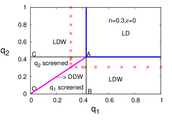
Let us now consider the phase diagram of the model in the plane for a fixed . Consider . Thus, is always satisfied, since . Therefore, the system can be only in LD or ID phases, but not in the HD phase for . For , the LD phase follows, else the ID phase ensues with a pair of DDWs are found along the line . For similar arguments follow, leading to the system showing only the HD or ID phase with no LD phase possible. The corresponding phase boundaries may be similarly obtained phase. This is consistent with the particle-hole symmetry of the model. For half filling (), both and yields , so that for , the ID phase prevails with DDWs along , with no LD/HD phases. More generally, as , the area covered by the ID phase in the phase diagram increases, covering the entire phase diagram for . Evidently, MFT and MCS results, though agree qualitatively, lack quantitative agreement, presumably due to the correlation effects neglected in MFT (see Fig. 3(a) above for equivalent quantitative disagreements between MFT and MCS results for density profiles). We have used various system sizes in our MCS studies, ranging from to 2000, all of which agree with each other within the numerical accuracies of our MCS studies, ruling out any significant system size effects. Notice that in region AOC (AOB) of Fig. 10, both satisfy ID phase condition, but is screened by . Now with the current for channels in the bulk, is clearly continuous across the phase boundaries in Fig. 10, since density changes continuously across the phase boundaries. This is reminiscent of a second order phase transition between the LD and ID phases (and hence between the HD and ID phases by using the particle-hole symmetry in the model). Equivalently, considering the LDW position as an order parameter, the phase boundaries in Fig. 10 are second order in nature, with an order parameter exponent 1. This may be obtained as follows: Assume (thus irrelevant). Then, to obtain the behavior of near the LD-ID phase transition, use Eq. (7) and set
| (19) |
with at the threshold of the ID phase for a given . This yields,
| (20) |
for small , where we have used Eq. (7 to obtain the above. Now, define an order parameter , such that it is zero in the LD phase and non-zero in the ID phase. For small , then, , giving the order parameter exponent 1, with as the control parameter (analog of ”temperature” in an equilibrium phase transition). This is in contrast to a typical mean-field value of 1/2 for the order parameter exponents in equilibrium systems [23].
V Conclusion and outlook
This work, thus, shows how the mutual interplay between PNC and bottleneck competition leads to a complex macroscopic behavior including delocalization transitions of LDWs and confinement of DDWs. While, coarse-grained measurements of an LDW (or DDWs) reveal the strength and (relative) position(s) of the strongest bottleneck(s), but screening prevents detecting the subdominant bottlenecks. Equivalently, different systems having the same particle density and strongest bottleneck(s), but with varying (in number, strength and relative positions) subdominant bottlenecks yield same macroscopic density profiles, revealing an underlying universal feature. This universal feature uncovered here has strong experimental implications. For instance, ribosome density mapping [24] or ribosome density profiling [25] experiments measuring coarse-grained densities can detect only the strongest pause sites (or non-preferred codons), but cannot resolve the other weaker (subdominant) pause sites. As we have already discussed above, the notion of universality in the present context is conceptually distinct from its implications elsewhere. We also take note of the fact that in our model particle number conservation affects the resulting macroscopic density profiles in ways that are very different from its role in other systems, e.g., universal critical dynamics in equilibrium or nonequilibrium systems. Phenomenologically, DDW confinements imply that tuning the bottleneck positions, it is possible to control the extent of movement of inhomogeneous densities, a feature expected to be significant for in-vitro set ups. Our results may be tested in in-vitro experiments by studying the restricted 1D motion of micron-sized self-propelled (active) particles along circular rings with constrictions [26]. In addition, general features of our results should be observed in vehicular jams in a closed network of roads with bottlenecks, e.g., in Formula 1 tracks where car speeds are reduced near the sharp bends (”bottleneck”), resulting into accumulation of cars behind them [27]. We now make a brief comparison between our results and those of Refs. [9, 10]. The latter works typically found localized shocks or LDW. In addition, Ref. [10] also found that a second, smaller bottleneck, far form the first one has no effect on the current. In particular in both Refs. [9, 10] the hopping rate across the defects (point of extended) have the same magnitude. Our closed model, in contrast, display DDWs in addition to LDWs, the associated localization-delocalization transitions and confinement of the DDWs. Furthermore, screening of the weaker defect in our model can happen regardless of the mutual distance between the weaker and the stronger defects. Note that in general we have unequal hopping rates at the point defects, unlike the models in Refs. [9, 10].
Our work is a promising starting point for understanding systems with a large number of discrete bottlenecks. For intermediate values of , macroscopically inhomogeneous density profiles ensue. With nonidentical bottlenecks, the strongest one, (i.e., with the lowest hopping rate) controls the macroscopic inhomogeneity in the form of an LDW, whose position may be obtained by above analysis together with screening of the weaker bottlenecks. When there are more than one strongest bottleneck, those many DDWs will be formed, as here. Nonetheless, screening of weaker bottlenecks and its experimental implications should generally hold. Our model is complementary to the model in Ref. [28]. It will be interesting to study how density profiles for discrete, isolated bottlenecks are modified eventually reducing to the results in Ref. [28]. Lastly, considering the central role of number conservation in the present model, it will be interesting to see how violations, especially weak violations of particle number conservation affect the steady states in this system [29].
VI Acknowledgement
One of the authors (AB) wishes to thank the Max-Planck-Gesellschaft (Germany) and Department of Science and Technology/Indo-German Science and Technology Centre (India) for partial financial support through the Partner Group programme (2009). NS would like to thank S. Biswas, A. Ghosh and A. Chandra for fruitful discussions.
Appendix A Mean-field Phase diagram in the plane
An analogous mean-field phase diagram in the () plane is shown in Fig. 11. The LD, HD and ID phases are shown; gives the boundary between the LD and ID phase; gives the boundary between the ID and HD phases. The upper limit of is confined up to , since above this value, gets screened by ; gives the location of DDWs. Not surprisingly, the particle current is continuous across the phase boundaries in Fig. 11, similar to the continuity of the particle current across the phase boundaries in Fig. 10. This is consistent with the second order phase transitions between the LD (HD) and the ID phases in the system.

Appendix B Locations of LDW and DDW in the plane
Consider the locations of LDW and DDWs in the plane, where with . Evidently, the line corresponds to DDWs in the model, with DDW spans shrinking as rises to 1, finally being fully confined at . The rest of the box with corresponds to LDWs in the system.

References
- [1] TASEP serves as a reduced model for a large class of natural phenomena involving geometric confinements in 1D, ranging from motion in nuclear pore complex of cells [I. Kosztin and K. Schulten, Phys. Rev. Lett. 93, 238102 (2004)], motion of molecular motors along microtubules [J. MacDonald, J. Gibbs and A. Pipkin, Biopolymers 6, 1 (1968); R. Lipowsky, S. Klump and T. M. Nieuwenhuizen, Phys. Rev. Lett. 87, 108101 (2001)], artificial crystalline zeolites [J. Kärger and D. Ruthven, Diffusion in Zeolites and other microporous solids (Wiley, New York, 1992)] to protein synthesis by messenger RNA (mRNA) ribosome complex in cells [Alberts book].
- [2] D. Chowdhury, L. Santen and A. Schadschneider , Phys. Rep. 329, 199 (2000); D. Helbing, Rev. Mod. Phys. 73, 1067 (2001).
- [3] B. Schmittmann and R. Zia, in Phase Transitions and Critical Phenomena, edited by C. Domb and J. Lebowitz (Academic Press, London, 1995).
- [4] T. Chou, K. Mallick and R. K. P. Zia, Rep. Prog. Phys. 74, 116601 (2011).
- [5] M. Liu et al, Phys. Lett. A, 373, 195 (2009).
- [6] Under certain conditions mRNA strands may form closed loops facilitating ribosome recycling, see, e.g., T. Chou, Biophys. J. 85, 755 (2003); S. E. Wells, E. Hillner, R. D. Vale and A. B. Sachs, Mol. Cell. 2, 135 (1998); S. Wang, K. S. Browning and W. A. Miller, EMBO J. 16, 4107 (1997).
- [7] Often there are sites along the mRNA chain at which ribosomes pause or slow down (defects). For instance, FMRP (a polyribosome-associated neuronal RNA-binding protein) can stall ribosome translocation, or, the slowdown of a translating ribosome upon encountering a rare codon in the mRNA due to the low concentration of the corresponding tRNA, see, e.g., Y. Nakamura, T. Gojobori, and T. Ikemura, Nucleic Acids Res. 28 292 (2000).
- [8] S. A. Janowsky and J. L. Lebowitz, Phys. Rev. A 45, 618 (1992).
- [9] J. J. Dong, B. Schmittmann, R. K. P. Zia, J. Stat. Phys. 128, 21 (2007).
- [10] P. Greulich and A. Schadschneider, Physica A 387. 1972 (2008).
- [11] R.K.P. Zia, J.J. Dong, and B. Schmittmann, J. Stat. Phys. 144, 405 (2011).
- [12] J. S. Nossan, J. Phys. A: Math. Theor. 46, 315001 (2013).
- [13] P. C. Hohenberg and B. I. Halperin, Rev. Mod. Phys. 49, 435 (1977).
- [14] D. Forster, D. R. Nelson and M. J. Stephen, Phys. Rev. A 16, 732 (1977).
- [15] TASEP with open boundaries does exhibit non-constant steady state density with equal entry and exit rates, both being less than 1/2. This has an analogue in the present model (see below).
- [16] P. Pierobon, et al, Phys. Rev. E, 74, 031906 (2006)
- [17] This is reasonable, for in the limit when any of , the system current must vanish. Thus, controls the bulk current in the ID phase of the system.
- [18] Interestingly, with , , i.e., the LDW is pushed to the the location of at For , , pushing the LDW in . This breaks down the basic MF assumption of splitting the system into and . However, an equivalent MF analysis may be constructed by considering the hole density . Since the holes move clockwise, an LDW will be formed that is entirely contained in and will be uniform with an LD phase for the holes. The MF hole density profiles may be found by following the MF analysis outlined above; the particle-hole symmetry then directly yields .
- [19] It may be noted that the use of the term ”screening” does not imply any collective effect here. It only refers to experimental invisibility (in a coarse-grained sense) of the weaker bottleneck in the presence of the stronger one.
- [20] This is equivalent to hypothetically replacing the actual DDW density profiles in and by two identical -functions at : .
- [21] For , from Eq. (8), , and hence, the DDW span is larger than or . However, as discussed in Ref. [18] above, MFT may still be constructed for the hole densities , such that the DDW span for the holes is smaller than . Particle-hole symmetry then allows us to calculate the corresponding DDW particle density profiles in the system.
- [22] In this limit, our model is identical to the one in Ref. [8].
- [23] See, e.g., P. M. Chaikin and T. C. Lubensky, Principles of condensed matter physics (Cambridge University Press, 2000).
- [24] Y. Arava et al, Nucl. Acids Res. 33, 2421 (2005).
- [25] N. T. Ingolia et al, Science 324, 218 (2009); H. Guo et al, Nature 466, 835 (2010).
- [26] F. Kümmel et al, Phys. Rev. Lett. 110, 198302 (2013).
- [27] See, e.g., http://en.espnf1.com/f1/motorsport/circuit/index.html?season=2012
- [28] G. Tripathy and M. Barma, Phys. Rev. E 58, 1911 (1998).
- [29] N. Sarkar, work in progress.