跳到论文正文
W Papers独立论文阅读器 arXiv:1403.0899 论文正文 计算阅读时间 · 0%
引用这篇论文根据当前论文元数据生成,正式投稿前建议核对。


License: arXiv.org perpetual non-exclusive license
arXiv:1403.0899v1 [math.DS] 04 Mar 2014

Introduction to Iterated Monodromy Groups

Sébastien Godillon
March 24, 2012
Abstract

The theory of iterated monodromy groups was developed by Nekrashevych [Nek05]. It is a wonderful example of application of group theory in dynamical systems and, in particular, in holomorphic dynamics. Iterated monodromy groups encode in a computationally efficient way combinatorial information about any dynamical system induced by a post-critically finite branched covering. Their power was illustrated by a solution of the Hubbard Twisted Rabbit Problem given by Bartholdi and Nekrashevych [BN06].

These notes attempt to introduce this theory for those who are familiar with holomorphic dynamics but not with group theory. The aims are to give all explanations needed to understand the main definition (Definition 3.2) and to provide skills in computing any iterated monodromy group efficiently (see examples in Section 3.3). Moreover some explicit links between iterated monodromy groups and holomorphic dynamics are detailed. In particular, Section 4.1 provides some facts about combinatorial equivalence classes, and Section 4.2 deals with matings of polynomials.

Representations of groups, automata, bimodules and virtual endomorphisms are intentionally omitted in order to make this introduction more elementary. All the proofs are mainly based on the path and homotopy lifting properties (Proposition 1.2) from algebraic topology. For further reading see [Pil03b], [Nek05] and [GŠ07].

These notes come from lectures given in the Chinese Academy of Sciences in Beijing in September 2011. The way to introduce iterated monodromy groups by using two trees (one left to label the vertices and one right for the edges, see Section 2) was explained to the author by Tan Lei although it implicitly appears in [Nek05] and some others works. The author would like very much to thank Laurent Bartholdi for his fruitful discussion and patience in explaining his works, the referee for his helpful comments and relevant suggestions and Tan Lei for her support and encouragement.

1 Preliminaries

1.1 Tree automorphism

A tree TT is a (simple undirected) graph which is connected and has no cycles. More precisely, a tree T=(V,E)T=(V,E) is the data of a set of vertices VV and a set of edges EE which are pairs of two distinct vertices, such that for any two distinct vertices v,v′v,v^{\prime} there is a unique path of edges from vv to v′v^{\prime}. For every edge {v,v′}\{v,v^{\prime}\}, the vertices vv and v′v^{\prime} are said to be adjacent which is denoted v∼Tv′v\stackrel{{\scriptstyle T}}{{\sim}}v^{\prime} (being adjacent is a symmetric binary relation).

A tree TT is said rooted if one vertex t∈Vt\in V has been designated the root. In this case, one can write the set of all vertices as the following partition V=⨆n⩾0VnV=\bigsqcup_{n\geqslant 0}V^{n} where VnV^{n} is the set of all the vertices linked to the root tt by a path of exactly nn edges (and V0={t}V^{0}=\{t\}). Each VnV^{n} is called the set of all vertices of level nn.

Definition 1


     Two rooted trees T=(V,E)T=(V,E) and T^=(V^,E^)\widehat{T}=(\widehat{V},\widehat{E}) are said to be isomorphic if there is a bijection φ\varphi from V=⨆n⩾0VnV=\bigsqcup_{n\geqslant 0}V^{n} onto V^=⨆n⩾0V^n\widehat{V}=\bigsqcup_{n\geqslant 0}\widehat{V}^{n} satisfying the following two axioms Level preserving: ∀n⩾0,φ⁡(Vn)=V^n\forall n\geqslant 0,\ \varphi(V^{n})=\widehat{V}^{n} Edge preserving: ∀v,v′∈V,v∼Tv′⇒φ⁡(v)∼T^φ⁡(v′)\forall v,v^{\prime}\in V,\ v\stackrel{{\scriptstyle T}}{{\sim}}v^{\prime}\Rightarrow\varphi(v)\stackrel{{\scriptstyle\widehat{T}}}{{\sim}}\varphi(v^{\prime}) Such a bijection φ\varphi is called a tree isomorphism. A tree automorphism is a tree isomorphism from a rooted tree TT onto itself. The set of all tree automorphisms of TT is denoted by Aut⁡(T)\Aut(T) and it is equipped with the group structure coming from composition of maps. For every pair of tree automorphisms g,hg,h in Aut⁡(T)\Aut(T), their composition is denoted by g.hg.h where the map gg is performed first (this notation is more convenient for computations in Aut⁡(T)\Aut(T) than h∘gh\circ g).


Given the alphabet ℰ={0,1,…,d−1}\mathcal{E}=\{0,1,\dots,d-1\} of d⩾2d\geqslant 2 letters, consider the following sets of words

  • •

    ℰ0={∅}\mathcal{E}^{0}=\{\emptyset\}

  • •

    ∀n⩾1,ℰn={words of length ​n​ with letters in ​ℰ}={ε1​ε2​…​εn/∀k,εk∈ℰ}\forall n\geqslant 1,\ \mathcal{E}^{n}=\{\text{words of length }n\text{ with letters in }\mathcal{E}\}=\{\varepsilon_{1}\varepsilon_{2}\dots\varepsilon_{n}\ /\ \forall k,\ \varepsilon_{k}\in\mathcal{E}\}

  • •

    ℰ⋆=⨆n⩾0ℰn\mathcal{E}^{\star}=\bigsqcup_{n\geqslant 0}\mathcal{E}^{n}

Definition 2


     The regular rooted tree TdT_{d} is defined as follows Root: the empty word ∅\emptyset Vertices: the set of words ℰ⋆=⨆n⩾0ℰn\mathcal{E}^{\star}=\bigsqcup_{n\geqslant 0}\mathcal{E}^{n} Edges: all the pairs {w,w​ε}\{w,w\varepsilon\} where ww is a word in ℰ⋆\mathcal{E}^{\star} and ε\varepsilon is a letter in ℰ\mathcal{E}


The graph below shows the first three levels of the regular rooted tree T2T_{2}.

000\textstyle{000\ignorespaces\ignorespaces\ignorespaces\ignorespaces\ignorespaces\ignorespaces\ignorespaces\ignorespaces}00\textstyle{00\ignorespaces\ignorespaces\ignorespaces\ignorespaces\ignorespaces\ignorespaces\ignorespaces\ignorespaces}001\textstyle{001\ignorespaces\ignorespaces\ignorespaces\ignorespaces\ignorespaces\ignorespaces\ignorespaces\ignorespaces}0\textstyle{0\ignorespaces\ignorespaces\ignorespaces\ignorespaces\ignorespaces\ignorespaces\ignorespaces\ignorespaces}010\textstyle{010\ignorespaces\ignorespaces\ignorespaces\ignorespaces\ignorespaces\ignorespaces\ignorespaces\ignorespaces}01\textstyle{01\ignorespaces\ignorespaces\ignorespaces\ignorespaces\ignorespaces\ignorespaces\ignorespaces\ignorespaces}011\textstyle{011\ignorespaces\ignorespaces\ignorespaces\ignorespaces\ignorespaces\ignorespaces\ignorespaces\ignorespaces}∅\textstyle{\emptyset\ignorespaces\ignorespaces\ignorespaces\ignorespaces\ignorespaces\ignorespaces\ignorespaces\ignorespaces}…\textstyle{\hskip 30.0pt\dots}100\textstyle{100\ignorespaces\ignorespaces\ignorespaces\ignorespaces\ignorespaces\ignorespaces\ignorespaces\ignorespaces}10\textstyle{10\ignorespaces\ignorespaces\ignorespaces\ignorespaces\ignorespaces\ignorespaces\ignorespaces\ignorespaces}101\textstyle{101\ignorespaces\ignorespaces\ignorespaces\ignorespaces\ignorespaces\ignorespaces\ignorespaces\ignorespaces}1\textstyle{1\ignorespaces\ignorespaces\ignorespaces\ignorespaces\ignorespaces\ignorespaces\ignorespaces\ignorespaces}110\textstyle{110\ignorespaces\ignorespaces\ignorespaces\ignorespaces\ignorespaces\ignorespaces\ignorespaces\ignorespaces}11\textstyle{11\ignorespaces\ignorespaces\ignorespaces\ignorespaces\ignorespaces\ignorespaces\ignorespaces\ignorespaces}111\textstyle{111\ignorespaces\ignorespaces\ignorespaces\ignorespaces\ignorespaces\ignorespaces\ignorespaces\ignorespaces}

The regular rooted tree TdT_{d} is an example of self-similar object. Namely for every word v∈ℰ⋆v\in\mathcal{E}^{\star}, the map φv:ℰ⋆→v​ℰ⋆,w↦v​w\varphi_{v}:\mathcal{E}^{\star}\rightarrow v\mathcal{E}^{\star},\ w\mapsto vw is a tree isomorphism from TdT_{d} onto the regular subtree Td|vT_{d}|_{v} rooted at vv.

For any tree automorphism g∈Aut⁡(Td)g\in\Aut(T_{d}) and any word v∈ℰ⋆v\in\mathcal{E}^{\star}, notice that the following map

ℛv​(g)=(φg⁡(v))−1∘g|v​ℰ⋆∘φv\mathcal{R}_{v}(g)=(\varphi_{g(v)})^{-1}\circ g|_{v\mathcal{E}^{\star}}\circ\varphi_{v}

is well defined from ℰ⋆\mathcal{E}^{\star} onto itself since the restriction g|v​ℰ⋆:v​ℰ⋆→g⁡(v)​ℰ⋆g|_{v\mathcal{E}^{\star}}:v\mathcal{E}^{\star}\rightarrow g(v)\mathcal{E}^{\star} is a tree isomorphism from the regular subtree Td|vT_{d}|_{v} rooted at vv onto the regular subtree Td|g⁡(v)T_{d}|_{g(v)} rooted at g⁡(v)g(v). Actually ℛv​(g)\mathcal{R}_{v}(g) defines a tree automorphism of TdT_{d} as it is shown in the commutative diagram below.

Td\textstyle{T_{d}\ignorespaces\ignorespaces\ignorespaces\ignorespaces\ignorespaces\ignorespaces\ignorespaces\ignorespaces}ℛv​(g)\scriptstyle{\textstyle\mathcal{R}_{v}(g)}φv\scriptstyle{\textstyle\varphi_{v}}Td\textstyle{T_{d}\ignorespaces\ignorespaces\ignorespaces\ignorespaces}φg⁡(v)\scriptstyle{\textstyle\varphi_{g(v)}}Td|v\textstyle{T_{d}|_{v}\ignorespaces\ignorespaces\ignorespaces\ignorespaces}g|v​ℰ⋆\scriptstyle{\textstyle g|_{v\mathcal{E}^{\star}}}Td|g⁡(v)\textstyle{T_{d}|_{g(v)}}

Definition 3


     For any tree automorphism g∈Aut⁡(Td)g\in\Aut(T_{d}) and any word v∈ℰ⋆v\in\mathcal{E}^{\star}, the following tree automorphism ℛv​(g)=(φg⁡(v))−1∘g|v​ℰ⋆∘φv\mathcal{R}_{v}(g)=(\varphi_{g(v)})^{-1}\circ g|_{v\mathcal{E}^{\star}}\circ\varphi_{v} is called the renormalization of gg at vv. A subgroup GG of Aut⁡(Td)\Aut(T_{d}) is said to be self-similar if the following condition holds ∀g∈G,∀v∈ℰ⋆,ℛv​(g)∈G\forall g\in G,\ \forall v\in\mathcal{E}^{\star},\ \mathcal{R}_{v}(g)\in G


Since φv∘φv′=φv​v′\varphi_{v}\circ\varphi_{v^{\prime}}=\varphi_{vv^{\prime}} for every pair of words v,v′v,v^{\prime} in ℰ⋆\mathcal{E}^{\star}, it follows that ℛv′​(ℛv​(g))=ℛv​v′​(g)\mathcal{R}_{v^{\prime}}\left(\mathcal{R}_{v}(g)\right)=\mathcal{R}_{vv^{\prime}}(g) for every tree automorphism g∈Aut⁡(Td)g\in\Aut(T_{d}). Therefore a quick induction shows that one only needs to check the condition above for words v∈ℰ⋆v\in\mathcal{E}^{\star} of length 11. That is

G​ is self-similar⟺∀g∈G,∀ε∈ℰ,ℛε​(g)∈GG\text{ is self-similar}\Longleftrightarrow\forall g\in G,\ \forall\varepsilon\in\mathcal{E},\ \mathcal{R}_{\varepsilon}(g)\in G
  • Example :

    One can remark that any tree automorphism g∈Aut⁡(Td)g\in\Aut(T_{d}) induces a permutation g|ℰ1g|_{\mathcal{E}^{1}} of ℰ1=ℰ\mathcal{E}^{1}=\mathcal{E}. Although it is not a one-to-one correspondence, one can conversely define a tree automorphism gσ∈Aut⁡(Td)g_{\sigma}\in\Aut(T_{d}) from a given permutation σ∈Sym⁡(ℰ)\sigma\in\Sym(\mathcal{E}) by gσ:ℰ⋆→ℰ⋆,ε1​ε2​…​εn↦σ⁡(ε1)​σ​(ε2)​…​σ​(εn)g_{\sigma}:\mathcal{E}^{\star}\rightarrow\mathcal{E}^{\star},\ \varepsilon_{1}\varepsilon_{2}\dots\varepsilon_{n}\mapsto\sigma(\varepsilon_{1})\sigma(\varepsilon_{2})\dots\sigma(\varepsilon_{n}). Such a tree automorphism satisfies gσ​(w​w′)=gσ​(w)​gσ​(w′)g_{\sigma}(ww^{\prime})=g_{\sigma}(w)g_{\sigma}(w^{\prime}) for every pair of words w,w′w,w^{\prime} in ℰ⋆\mathcal{E}^{\star}. Therefore every renormalization of gσg_{\sigma} is equal to gσg_{\sigma} and any subgroup of Aut⁡(Td)\Aut(T_{d}) generated by such tree automorphisms induced by some permutations of ℰ\mathcal{E} is self-similar.

Remark that every tree automorphism g∈Aut⁡(Td)g\in\Aut(T_{d}) satisfies

∀ε∈ℰ,∀w∈ℰ⋆,g⁡(ε​w)=(g|ℰ1​(ε))​(ℛε​(g)​(w))\forall\varepsilon\in\mathcal{E},\forall w\in\mathcal{E}^{\star},\ g(\varepsilon w)=\Big(g|_{\mathcal{E}^{1}}(\varepsilon)\Big)\Big(\mathcal{R}_{\varepsilon}(g)(w)\Big)

Consequently any tree automorphism is entirely described by its renormalizations at every vertex in the first level together with its restriction on the first level which describes how the regular subtrees rooted at every vertex in the first level are interchanged. That provides a convenient way to encode tree automorphisms in order to make computations in Aut⁡(Td)\Aut(T_{d}).

Definition 4


     Every tree automorphism g∈Aut⁡(Td)g\in\Aut(T_{d}) may be uniquely written as follows g=σg​⟨⟨g0,g1,…,gd−1⟩⟩g=\sigma_{g}{\langle\!\langle}g_{0},g_{1},\dots,g_{d-1}{\rangle\!\rangle} where • σg=g|ℰ1∈Sym⁡(ℰ)\sigma_{g}=g|_{\mathcal{E}^{1}}\in\Sym(\mathcal{E}) is called the root permutation of gg • and for every letter ε∈ℰ\varepsilon\in\mathcal{E}, gε=ℛε​(g)∈Aut⁡(Td)g_{\varepsilon}=\mathcal{R}_{\varepsilon}(g)\in\Aut(T_{d}) is the renormalization of gg at ε\varepsilon This decomposition is called the wreath recursion of gg.


More precisely the map g↦(g|ℰ1,(ℛ0​(g),ℛ1​(g),…,ℛd−1​(g)))g\mapsto\left(g|_{\mathcal{E}^{1}},\left(\mathcal{R}_{0}(g),\mathcal{R}_{1}(g),\dots,\mathcal{R}_{d-1}(g)\right)\right) is a group isomorphism from Aut⁡(Td)\Aut(T_{d}) onto the semi-direct product Sym⁡(ℰ)⋉(Aut⁡(Td))d\Sym(\mathcal{E})\ltimes(\Aut(T_{d}))^{d} called the permutational wreath product (its binary operation is described below). Remark that a subgroup GG of Aut⁡(Td)\Aut(T_{d}) is said self-similar if and only if its image under this group isomorphism is a subgroup of Sym⁡(ℰ)⋉Gd\Sym(\mathcal{E})\ltimes G^{d}.

It is more convenient to think wreath recursion as in the graph below.

0\textstyle{0\ignorespaces\ignorespaces\ignorespaces\ignorespaces}g0\scriptstyle{\textstyle g_{0}}σg​(0)\textstyle{\sigma_{g}(0)}1\textstyle{1\ignorespaces\ignorespaces\ignorespaces\ignorespaces}g1\scriptstyle{\textstyle g_{1}}σg​(1)\textstyle{\sigma_{g}(1)}…\textstyle{\dots}…\textstyle{\dots}d−1\textstyle{d-1\ignorespaces\ignorespaces\ignorespaces\ignorespaces}gd−1\scriptstyle{\textstyle g_{d-1}}σg​(d−1)\textstyle{\sigma_{g}(d-1)}

Be aware that each arrow does not depict the map on its label. In fact, all the arrows describe the root permutation σg\sigma_{g} whereas the labels correspond to the renormalizations of gg. In practice the arrows are often “tied” to sort out the image on the right-hand side in the same order as on the left-hand side. The root permutation σg\sigma_{g} is then described by intertwined arrows. Furthermore a label is often forgotten if the corresponding renormalization is the identity tree automorphism Id∈Aut⁡(Td)\Id\in\Aut(T_{d}).

This kind of graph provides an easy way to compute with wreath recursions. Namely for every pair of tree automorphisms g,hg,h in Aut⁡(Td)\Aut(T_{d}), one get

0\textstyle{0\ignorespaces\ignorespaces\ignorespaces\ignorespaces}g0\scriptstyle{\textstyle g_{0}}σg​(0)\textstyle{\sigma_{g}(0)\ignorespaces\ignorespaces\ignorespaces\ignorespaces}hσg​(0)\scriptstyle{\textstyle h_{\sigma_{g}(0)}}σh​(σg​(0))\textstyle{\sigma_{h}(\sigma_{g}(0))}1\textstyle{1\ignorespaces\ignorespaces\ignorespaces\ignorespaces}g1\scriptstyle{\textstyle g_{1}}σg​(1)\textstyle{\sigma_{g}(1)\ignorespaces\ignorespaces\ignorespaces\ignorespaces}hσg​(1)\scriptstyle{\textstyle h_{\sigma_{g}(1)}}σh​(σg​(1))\textstyle{\sigma_{h}(\sigma_{g}(1))}…\textstyle{\dots}…\textstyle{\dots}…\textstyle{\dots}d−1\textstyle{d-1\ignorespaces\ignorespaces\ignorespaces\ignorespaces}gd−1\scriptstyle{\textstyle g_{d-1}}σg​(d−1)\textstyle{\sigma_{g}(d-1)\ignorespaces\ignorespaces\ignorespaces\ignorespaces}hσg​(d−1)\scriptstyle{\textstyle h_{\sigma_{g}(d-1)}}σh​(σg​(d−1))\textstyle{\sigma_{h}(\sigma_{g}(d-1))}

Lemma 1


     The wreath recursion of a composition of two tree automorphism g,hg,h in Aut⁡(Td)\Aut(T_{d}) is given by g.h=(σh∘σg)⟨⟨g0.hσg​(0),g1.hσg​(1),…,gd−1.hσg​(d−1)⟩⟩g.h=(\sigma_{h}\circ\sigma_{g}){\Big\langle\!\Big\langle}g_{0}.h_{\sigma_{g}(0)},g_{1}.h_{\sigma_{g}(1)},\dots,g_{d-1}.h_{\sigma_{g}(d-1)}{\Big\rangle\!\Big\rangle} In particular, the inverse wreath recursion of a tree automorphism gg in Aut⁡(Td)\Aut(T_{d}) is given by g−1=σg−1​⟨⟨gσg−1​(0)−1,gσg−1​(1)−1,…,gσg−1​(d−1)−1⟩⟩g^{-1}=\sigma_{g}^{-1}{\Big\langle\!\Big\langle}g_{\sigma_{g}^{-1}(0)}^{-1},g_{\sigma_{g}^{-1}(1)}^{-1},\dots,g_{\sigma_{g}^{-1}(d-1)}^{-1}{\Big\rangle\!\Big\rangle}


  • Example - the adding machine :

    Every word in ℰ⋆\mathcal{E}^{\star} may be thought as a dd-ary integer whose digits are written from left to right. Let g∈Aut⁡(Td)g\in\Aut(T_{d}) be the adding machine on ℰ⋆\mathcal{E}^{\star}, namely the process of adding one to the left most digit of every dd-ary integer (with the convention that adding one to the word 11​…​1∈ℰn11\dots 1\in\mathcal{E}^{n} gives the word 00​…​0∈ℰn00\dots 0\in\mathcal{E}^{n} of same length). More precisely, the adding machine gg is recursively defined by

    ∀ε∈ℰ,∀w∈ℰ⋆,g⁡(ε​w)={(ε+1)​wif ​ε∈{0,1,…,d−2}0​g​(w)if ​ε=d−1\forall\varepsilon\in\mathcal{E},\forall w\in\mathcal{E}^{\star},\ g(\varepsilon w)=\left\{\begin{array}[]{ll}(\varepsilon+1)w&\text{if }\varepsilon\in\{0,1,\dots,d-2\}\\ 0g(w)&\text{if }\varepsilon=d-1\end{array}\right.

    Then gg may be seen as the wreath recursion g=σ⁡⟨⟨Id,Id,…,Id,g⟩⟩g=\sigma{\langle\!\langle}\Id,\Id,\dots,\Id,g{\rangle\!\rangle} where σ\sigma is the cyclic permutation such that σ⁡(ε)=ε+1\sigma(\varepsilon)=\varepsilon+1 if ε∈{0,1,…,d−2}\varepsilon\in\{0,1,\dots,d-2\} and σ⁡(d−1)=0\sigma(d-1)=0, namely σ=(0,1,…,d−1)\sigma=(0,1,\dots,d-1) (using circular notation).

    0\textstyle{0\ignorespaces\ignorespaces\ignorespaces\ignorespaces}0\textstyle{0}1\textstyle{1\ignorespaces\ignorespaces\ignorespaces\ignorespaces}1\textstyle{1}…\textstyle{\dots}2\textstyle{2}d−2\textstyle{d-2\ignorespaces\ignorespaces\ignorespaces\ignorespaces}…\textstyle{\dots}d−1\textstyle{d-1\ignorespaces\ignorespaces\ignorespaces\ignorespaces\ignorespaces\ignorespaces}g\scriptstyle{\textstyle g}d−1\textstyle{d-1}

    Lemma 1.1 allows to compute easily the inverse wreath recursion g−1=σ−1​⟨⟨g−1,Id,…,Id⟩⟩g^{-1}=\sigma^{-1}{\langle\!\langle}g^{-1},\Id,\dots,\Id{\rangle\!\rangle} since

    0\textstyle{0\ignorespaces\ignorespaces\ignorespaces\ignorespaces}0\textstyle{0\ignorespaces\ignorespaces\ignorespaces\ignorespaces\ignorespaces\ignorespaces}g−1\scriptstyle{\textstyle g^{-1}}0\textstyle{0}1\textstyle{1\ignorespaces\ignorespaces\ignorespaces\ignorespaces}1\textstyle{1\ignorespaces\ignorespaces\ignorespaces\ignorespaces}1\textstyle{1}…\textstyle{\dots}2\textstyle{2\ignorespaces\ignorespaces\ignorespaces\ignorespaces}…\textstyle{\dots}d−2\textstyle{d-2\ignorespaces\ignorespaces\ignorespaces\ignorespaces}…\textstyle{\dots}d−2\textstyle{d-2}d−1\textstyle{d-1\ignorespaces\ignorespaces\ignorespaces\ignorespaces\ignorespaces\ignorespaces}g\scriptstyle{\textstyle g}d−1\textstyle{d-1\ignorespaces\ignorespaces\ignorespaces\ignorespaces}d−1\textstyle{d-1}

    gives after “untying”

    0\textstyle{0\ignorespaces\ignorespaces\ignorespaces\ignorespaces}0\textstyle{0}1\textstyle{1\ignorespaces\ignorespaces\ignorespaces\ignorespaces}1\textstyle{1}…\textstyle{\dots}…\textstyle{\dots}d−2\textstyle{d-2\ignorespaces\ignorespaces\ignorespaces\ignorespaces}d−2\textstyle{d-2}d−1\textstyle{d-1\ignorespaces\ignorespaces\ignorespaces\ignorespaces}g.g−1=Id\scriptstyle{\textstyle g.g^{-1}=\Id}d−1\textstyle{d-1}

    A similar computation gives gd=⟨⟨g,g,…,g⟩⟩g^{d}={\langle\!\langle}g,g,\dots,g{\rangle\!\rangle}, and thus a quick induction shows that the adding machine acts as a cyclic permutation of order dnd^{n} on the nn-th level of TdT_{d} for every n⩾1n\geqslant 1.

  • Example - Hanoi Towers group (due to Grigorchuk and S̆unić [GŠ07])) :

    The popular Towers of Hanoi Problem deals with three rods and a given number nn of disks of different sizes which can slide onto every rod. The problem starts with all the disks in ascending order of size on one rod making a conical shape (see Figure 1), and consists to move the entire stack to another rod with respect to the following rules

    1. 1.

      Only one disk may be moved at a time.

    2. 2.

      Each move consists of taking the upper disk from one of the rods and sliding it onto another rod, on top of the other disks that may already be present on that rod.

    3. 3.

      No disk may be placed on top of a smaller disk.

    Refer to caption
    Figure 1: The starting configuration 0000 for the Hanoi Towers with four disks

    If the nn disks 1,2,…,n1,2,\dots,n are labeled with their size (11 being the smallest and nn the largest) and each rod is labeled with one letter from the alphabet ℰ={0,1,2}\mathcal{E}=\{0,1,2\}, then every word w=ε1​ε2​…​εn∈ℰnw=\varepsilon_{1}\varepsilon_{2}\dots\varepsilon_{n}\in\mathcal{E}^{n} of length nn encodes a unique configuration of the problem in which the kk-th disk is placed on the rod εk\varepsilon_{k} (and then the order of disks on any rod is determined by their size). Figure 1 and Figure 2 depict the starting configuration 0000∈ℰ40000\in\mathcal{E}^{4} and the configuration 1210∈ℰ41210\in\mathcal{E}^{4} for n=4n=4 disks.

    Refer to caption
    Figure 2: The configuration 1210 for the Hanoi Towers with four disks

    It turns out that each move between two rods is represented by either of the following wreath recursions

    a=(1,2)​⟨⟨a,Id,Id⟩⟩a=(1,2){\langle\!\langle}a,\Id,\Id{\rangle\!\rangle} b=(0,1)​⟨⟨Id,Id,b⟩⟩b=(0,1){\langle\!\langle}\Id,\Id,b{\rangle\!\rangle} c=(0,2)​⟨⟨Id,c,Id⟩⟩c=(0,2){\langle\!\langle}\Id,c,\Id{\rangle\!\rangle}
    for a move for a move for a move
    between rods 11 and 22 between rods 00 and 11 between rods 00 and 22
    0\textstyle{0\ignorespaces\ignorespaces\ignorespaces\ignorespaces}a\scriptstyle{\textstyle a}0\textstyle{0}1\textstyle{1\ignorespaces\ignorespaces\ignorespaces\ignorespaces}1\textstyle{1}2\textstyle{2\ignorespaces\ignorespaces\ignorespaces\ignorespaces}2\textstyle{2} 0\textstyle{0\ignorespaces\ignorespaces\ignorespaces\ignorespaces}0\textstyle{0}1\textstyle{1\ignorespaces\ignorespaces\ignorespaces\ignorespaces}1\textstyle{1}2\textstyle{2\ignorespaces\ignorespaces\ignorespaces\ignorespaces}b\scriptstyle{\textstyle b}2\textstyle{2} 0\textstyle{0\ignorespaces\ignorespaces\ignorespaces\ignorespaces\ignorespaces\ignorespaces}0\textstyle{0}1\textstyle{1\ignorespaces\ignorespaces\ignorespaces\ignorespaces}c\scriptstyle{\textstyle c}1\textstyle{1}2\textstyle{2\ignorespaces\ignorespaces\ignorespaces\ignorespaces\ignorespaces\ignorespaces}2\textstyle{2}

    For instance, one can go from the starting position 0000 in Figure 1 to the position 1210 in Figure 2 by the following sequence of basic moves between two rods

    b→c→a→b→ab\rightarrow c\rightarrow a\rightarrow b\rightarrow a

    In terms of wreath recursions, that gives

    0\textstyle{0\ignorespaces\ignorespaces\ignorespaces\ignorespaces}0\textstyle{0\ignorespaces\ignorespaces\ignorespaces\ignorespaces\ignorespaces\ignorespaces}0\textstyle{0\ignorespaces\ignorespaces\ignorespaces\ignorespaces}a\scriptstyle{\textstyle a}0\textstyle{0\ignorespaces\ignorespaces\ignorespaces\ignorespaces}0\textstyle{0\ignorespaces\ignorespaces\ignorespaces\ignorespaces}a\scriptstyle{\textstyle a}0\textstyle{0}1\textstyle{1\ignorespaces\ignorespaces\ignorespaces\ignorespaces}1\textstyle{1\ignorespaces\ignorespaces\ignorespaces\ignorespaces}c\scriptstyle{\textstyle c}1\textstyle{1\ignorespaces\ignorespaces\ignorespaces\ignorespaces}1\textstyle{1\ignorespaces\ignorespaces\ignorespaces\ignorespaces}1\textstyle{1\ignorespaces\ignorespaces\ignorespaces\ignorespaces}1\textstyle{1}2\textstyle{2\ignorespaces\ignorespaces\ignorespaces\ignorespaces}b\scriptstyle{\textstyle b}2\textstyle{2\ignorespaces\ignorespaces\ignorespaces\ignorespaces\ignorespaces\ignorespaces}2\textstyle{2\ignorespaces\ignorespaces\ignorespaces\ignorespaces}2\textstyle{2\ignorespaces\ignorespaces\ignorespaces\ignorespaces}b\scriptstyle{\textstyle b}2\textstyle{2\ignorespaces\ignorespaces\ignorespaces\ignorespaces}2\textstyle{2}

    or shortly after “untying”: b.c.a.b.a=(0,1)⟨⟨c.b,a,b.a⟩⟩b.c.a.b.a=(0,1){\langle\!\langle}c.b,a,b.a{\rangle\!\rangle}

    0\textstyle{0\ignorespaces\ignorespaces\ignorespaces\ignorespaces}c.b\scriptstyle{\textstyle c.b}0\textstyle{0}1\textstyle{1\ignorespaces\ignorespaces\ignorespaces\ignorespaces}a\scriptstyle{\textstyle a}1\textstyle{1}2\textstyle{2\ignorespaces\ignorespaces\ignorespaces\ignorespaces}b.a\scriptstyle{\textstyle b.a}2\textstyle{2}

    The Hanoi Towers group ℋ\mathcal{H} is defined to be the subgroup of Aut⁡(T3)\Aut(T_{3}) generated by the wreath recursions a,b,ca,b,c. It follows that the Towers of Hanoi Problem is equivalent to find an element gg in the Hanoi Tower group ℋ=⟨a,b,c⟩\mathcal{H}=\langle a,b,c\rangle (that is a sequence of basic moves between two rods) such that the image of the starting configuration (the word 00​…​0∈ℰn00\dots 0\in\mathcal{E}^{n}) is a goal configuration: g⁡(00​…​0)=11​…​1​ or ​22​…​2g(00\dots 0)=11\dots 1\text{ or }22\dots 2.

    Furthermore remark that the Hanoi Towers group ℋ\mathcal{H} is self-similar since every renormalization of the wreath recursions a,b,ca,b,c is either a,b,ca,b,c or Id\Id.

The following lemma is often used to prove that a given tree automorphism is actually equal to the identity tree automorphism. Indeed it may happen although its wreath recursion is not trivial. For instance, it turns out that the wreath recursion g=⟨⟨g,g,…,g⟩⟩g={\langle\!\langle}g,g,\dots,g{\rangle\!\rangle} is actually the identity tree automorphism Id∈Aut⁡(Td)\Id\in\Aut(T_{d}) (for instance by applying lemma below).

Lemma 2


     Let g1,g2,…,gmg_{1},g_{2},\dots,g_{m} be m⩾1m\geqslant 1 tree automorphisms in Aut⁡(Td)\Aut(T_{d}) such that • every root permutation σgk=gk|ℰ1\sigma_{g_{k}}=g_{k}|_{\mathcal{E}^{1}} is the identity permutation on the the alphabet ℰ\mathcal{E} • and every renormalization gk,ε=ℛε​(gk)g_{k,\varepsilon}=\mathcal{R}_{\varepsilon}(g_{k}) belongs to the subgroup of Aut⁡(Td)\Aut(T_{d}) generated by g1,g2,…,gmg_{1},g_{2},\dots,g_{m} In terms of wreath recursions, g1,g2,…,gmg_{1},g_{2},\dots,g_{m} are assumed to be written as follows {g1=⟨⟨g1,0,g1,1,…,g1,d−1⟩⟩g2=⟨⟨g2,0,g2,1,…,g2,d−1⟩⟩…gm=⟨⟨gm,0,gm,1,…,gm,d−1⟩⟩where∀k,∀ε∈ℰ,gk,ε∈⟨g1,g2,…,gm⟩\left\{\begin{array}[]{rcl}g_{1}&=&{\langle\!\langle}g_{1,0},g_{1,1},\dots,g_{1,d-1}{\rangle\!\rangle}\\ g_{2}&=&{\langle\!\langle}g_{2,0},g_{2,1},\dots,g_{2,d-1}{\rangle\!\rangle}\\ &\dots&\\ g_{m}&=&{\langle\!\langle}g_{m,0},g_{m,1},\dots,g_{m,d-1}{\rangle\!\rangle}\end{array}\right.\quad\text{where}\quad\forall k,\forall\varepsilon\in\mathcal{E},\ g_{k,\varepsilon}\in\Big\langle g_{1},g_{2},\dots,g_{m}\Big\rangle Then g1,g2,…,gmg_{1},g_{2},\dots,g_{m} are all equal to the identity tree automorphism Id∈Aut⁡(Td)\Id\in\Aut(T_{d}).


  • Proof  :

    Let n⩾2n\geqslant 2 be an integer and assume by induction that every gkg_{k} acts as the identity on the set of all words of lenght n−1n-1. Let w=ε1​ε2​…​εn∈ℰ⋆w=\varepsilon_{1}\varepsilon_{2}\dots\varepsilon_{n}\in\mathcal{E}^{\star} be a word of length nn. The image of ww under any tree automorphism gkg_{k} may be written as follows

    gk​(w)=gk​(ε1​ε2​…​εn)=(gk|ℰ1​(ε1))​(ℛε1​(gk)​(ε2​…​εn))=(σgk​(ε1))​(gk,ε1​(ε2​…​εn))g_{k}(w)=g_{k}(\varepsilon_{1}\varepsilon_{2}\dots\varepsilon_{n})=\Big(g_{k}|_{\mathcal{E}^{1}}(\varepsilon_{1})\Big)\Big(\mathcal{R}_{\varepsilon_{1}}(g_{k})(\varepsilon_{2}\dots\varepsilon_{n})\Big)=\Big(\sigma_{g_{k}}(\varepsilon_{1})\Big)\Big(g_{k,\varepsilon_{1}}(\varepsilon_{2}\dots\varepsilon_{n})\Big)

    The first assumption gives σgk​(ε1)=ε1\sigma_{g_{k}}(\varepsilon_{1})=\varepsilon_{1}. Furthermore it follows from the second assumption and from the inductive hypothesis that gk,ε1​(ε2​…​εn)=ε2​…​εng_{k,\varepsilon_{1}}(\varepsilon_{2}\dots\varepsilon_{n})=\varepsilon_{2}\dots\varepsilon_{n} since ε2​…​εn\varepsilon_{2}\dots\varepsilon_{n} is a word of length n−1n-1. Finally gk​(w)=(ε1)​(ε2​…​εn)=wg_{k}(w)=(\varepsilon_{1})(\varepsilon_{2}\dots\varepsilon_{n})=w and the result follows by induction (the inductive start is given by the first assumption).


In practice, to show that a given tree automorphism g∈Aut⁡(Td)g\in\Aut(T_{d}) is actually the identity tree automorphism, the aim is to find together with g=g1g=g_{1} some tree automorphisms g2,…,gmg_{2},\dots,g_{m} which satisfy assumptions from Lemma 1.1.

1.2 Partial self-covering

Definition 5


     Let ℳ\mathcal{M} be a path connected and locally path connected topological space. A partial self-covering of ℳ\mathcal{M} is a degree d⩾2d\geqslant 2 covering p:ℳ1→ℳp:\mathcal{M}_{1}\rightarrow\mathcal{M} where ℳ1⊆ℳ\mathcal{M}_{1}\subseteq\mathcal{M}. A partial self-covering can be iterated and the iterates, denoted by pn:ℳn→ℳp^{n}:\mathcal{M}_{n}\rightarrow\mathcal{M} where ℳn=p−n​(ℳ)⊆ℳ\mathcal{M}_{n}=p^{-n}(\mathcal{M})\subseteq\mathcal{M}, are also partial self-coverings. …\textstyle{\dots\ignorespaces\ignorespaces\ignorespaces\ignorespaces}ℳ3\textstyle{\mathcal{M}_{3}\ignorespaces\ignorespaces\ignorespaces\ignorespaces}p\scriptstyle{\textstyle p}ℳ2\textstyle{\mathcal{M}_{2}\ignorespaces\ignorespaces\ignorespaces\ignorespaces}p\scriptstyle{\textstyle p}ℳ1\textstyle{\mathcal{M}_{1}\ignorespaces\ignorespaces\ignorespaces\ignorespaces}p\scriptstyle{\textstyle p}ℳ\textstyle{\mathcal{M}}


  • Examples :

    Let ff be a post-critically finite branched covering map on the topological sphere 𝕊2\mathbb{S}^{2} and denote by PfP_{f} its post-critical set. Since Pf⊂f−1​(Pf)P_{f}\subset f^{-1}(P_{f}), ff induces the following partial self-covering.

    f:ℳ1=𝕊2\f−1​(Pf)⟶ℳ=𝕊2\Pff:\mathcal{M}_{1}=\mathbb{S}^{2}\backslash f^{-1}(P_{f})\longrightarrow\mathcal{M}=\mathbb{S}^{2}\backslash P_{f}

    The same holds for post-critically finite rational maps on the Riemann sphere ℂ^\widehat{\mathbb{C}} or for post-critically finite polynomials map on the complex plane ℂ\mathbb{C}.

Recall that a partial self-covering satisfies the following path and homotopy lifting properties.

Proposition 1


     (1) For every path ℓ\ell in ℳ\mathcal{M} with base point ℓ⁡(0)=t∈ℳ\ell(0)=t\in\mathcal{M} and any preimage x∈p−1​(t)x\in p^{-1}(t), there exists a unique path ℒx\mathscr{L}_{x} in ℳ1\mathcal{M}_{1} with base point ℒx​(0)=x\mathscr{L}_{x}(0)=x such that p∘ℒx=ℓp\circ\mathscr{L}_{x}=\ell (see the commutative diagram below). ℒx\mathscr{L}_{x} is called the pp-lift of ℓ\ell from xx. [0,1]\textstyle{[0,1]\ignorespaces\ignorespaces\ignorespaces\ignorespaces\ignorespaces\ignorespaces\ignorespaces\ignorespaces}ℒx\scriptstyle{\textstyle\mathscr{L}_{x}}ℓ\scriptstyle{\textstyle\ell}ℳ1\textstyle{\mathcal{M}_{1}\ignorespaces\ignorespaces\ignorespaces\ignorespaces}p\scriptstyle{\textstyle p}ℳ\textstyle{\mathcal{M}} (2) Furthermore if l:[0,1]×[0,1]→ℳl:[0,1]\times[0,1]\rightarrow\mathcal{M} is a homotopy of paths with l(0,.)=ℓl(0,.)=\ell then there exists a unique homotopy of paths Lx:[0,1]×[0,1]→ℳ1L_{x}:[0,1]\times[0,1]\rightarrow\mathcal{M}_{1} such that Lx(s,.)L_{x}(s,.) is the pp-lift of l(s,.)l(s,.) from l⁡(s,0)l(s,0) for every s∈[0,1]s\in[0,1] (in particular Lx(0,.)=ℒxL_{x}(0,.)=\mathscr{L}_{x} for s=0s=0). (3) Therefore for every loop γ\gamma in ℳ\mathcal{M} with base point ℓ⁡(0)=t∈ℳ\ell(0)=t\in\mathcal{M} and any preimage x∈p−1​(t)x\in p^{-1}(t), the terminal point y=Γx​(1)y=\Gamma_{x}(1) of the pp-lift Γx\Gamma_{x} of γ\gamma from xx depends on γ\gamma only through its homotopy class [γ]∈π1​(ℳ,t)[\gamma]\in\pi_{1}(\mathcal{M},t). Since yy is also a preimage of tt under pp, it turns out that the fundamental group π1​(ℳ,t)\pi_{1}(\mathcal{M},t) acts on p−1​(t)p^{-1}(t) by [γ]​x=Γx​(1)[\gamma]x=\Gamma_{x}(1). x\textstyle{x\ignorespaces\ignorespaces\ignorespaces\ignorespaces\ignorespaces\ignorespaces\ignorespaces\ignorespaces}Γx\scriptstyle{\textstyle\Gamma_{x}}p\scriptstyle{\textstyle p}t\textstyle{t\ignorespaces\ignorespaces\ignorespaces\ignorespaces\ignorespaces\ignorespaces}[γ]\scriptstyle{\textstyle[\gamma]}y\textstyle{y\ignorespaces\ignorespaces\ignorespaces\ignorespaces}p\scriptstyle{\textstyle p}


The same holds for pn:ℳn→ℳp^{n}:\mathcal{M}_{n}\rightarrow\mathcal{M} as well, namely the fundamental group π1​(ℳ,t)\pi_{1}(\mathcal{M},t) acts on the set of preimages p−n​(t)p^{-n}(t) by [γ]​x=Γx​(1)[\gamma]x=\Gamma_{x}(1) where Γx\Gamma_{x} is the pnp^{n}-lift of γ\gamma from xx.

2 Tree of preimages

Let p:ℳ1→ℳp:\mathcal{M}_{1}\rightarrow\mathcal{M} be a partial self-covering of degree d⩾2d\geqslant 2 and tt be a point in ℳ\mathcal{M}.

2.1 A right-hand tree

Definition 6


     The (right-hand) tree of preimages T⁡(p,t)T(p,t) is the rooted tree defined as follows Root: the point tt Vertices: the abstract set of preimages ⨆n⩾0p−n​(t)\bigsqcup_{n\geqslant 0}p^{-n}(t) Edges: all the pairs {p⁡(x),x}\{p(x),x\} where p​(x)∈p−n​(t)p(x)\in p^{-n}(t) and x∈p−(n+1)​(t)x\in p^{-(n+1)}(t) for some n⩾0n\geqslant 0 By “abstract set”, one distinguishes a same point that belongs to two distinct levels. More precisely, some preimages corresponding to distinct levels may coincide in ℳ1\mathcal{M}_{1} but are distinguished in T⁡(p,t)T(p,t) (in particular every edge is well defined).


The graph below shows the first levels of a tree of preimages of a degree d=2d=2 partial self-covering.

p\scriptstyle{p}p\scriptstyle{p}p\scriptstyle{p}p\scriptstyle{p}p\scriptstyle{p}p\scriptstyle{p}t\textstyle{t\ignorespaces\ignorespaces\ignorespaces\ignorespaces\ignorespaces\ignorespaces\ignorespaces\ignorespaces}p\scriptstyle{p}p\scriptstyle{p}…\textstyle{\hskip 30.0pt\dots}p\scriptstyle{p}p\scriptstyle{p}p\scriptstyle{p}p\scriptstyle{p}p\scriptstyle{p}p\scriptstyle{p}
  • Example :

    Consider the degree d=2d=2 partial self-covering Q0:ℂ\{0}→ℂ\{0},z↦z2Q_{0}:\mathbb{C}\backslash\{0\}\rightarrow\mathbb{C}\backslash\{0\},\ z\mapsto z^{2} and let t=1t=1 be the root. The first two levels of the tree of preimages T⁡(Q0,1)T(Q_{0},1) are then

    1\textstyle{1\ignorespaces\ignorespaces\ignorespaces\ignorespaces\ignorespaces\ignorespaces\ignorespaces\ignorespaces}Q0\scriptstyle{Q_{0}}Q0\scriptstyle{Q_{0}}1\textstyle{1\ignorespaces\ignorespaces\ignorespaces\ignorespaces\ignorespaces\ignorespaces\ignorespaces\ignorespaces}Q0\scriptstyle{Q_{0}}Q0\scriptstyle{Q_{0}}−1\textstyle{-1\ignorespaces\ignorespaces\ignorespaces\ignorespaces\ignorespaces\ignorespaces\ignorespaces\ignorespaces}Q0\scriptstyle{Q_{0}}Q0\scriptstyle{Q_{0}}t=1\textstyle{t=1\ignorespaces\ignorespaces\ignorespaces\ignorespaces\ignorespaces\ignorespaces\ignorespaces\ignorespaces}Q0\scriptstyle{Q_{0}}Q0\scriptstyle{Q_{0}}…\textstyle{\hskip 30.0pt\dots}i\textstyle{i\ignorespaces\ignorespaces\ignorespaces\ignorespaces\ignorespaces\ignorespaces\ignorespaces\ignorespaces}Q0\scriptstyle{Q_{0}}Q0\scriptstyle{Q_{0}}−1\textstyle{-1\ignorespaces\ignorespaces\ignorespaces\ignorespaces\ignorespaces\ignorespaces\ignorespaces\ignorespaces}Q0\scriptstyle{Q_{0}}Q0\scriptstyle{Q_{0}}−i\textstyle{-i\ignorespaces\ignorespaces\ignorespaces\ignorespaces\ignorespaces\ignorespaces\ignorespaces\ignorespaces}Q0\scriptstyle{Q_{0}}Q0\scriptstyle{Q_{0}}

It turns out that the tree of preimages T⁡(p,t)T(p,t) of a degree dd partial self-covering is isomorphic to the regular rooted tree TdT_{d}. However there is no canonical choice for a tree isomorphism between them. Actually Definition 2.1 does not provide a canonical labeling of all vertices of T⁡(p,t)T(p,t).

2.2 A left-hand tree

Definition 7


     A labeling choice (L)(L) for the partial covering p:ℳ1→ℳp:\mathcal{M}_{1}\rightarrow\mathcal{M} and the base point t∈ℳt\in\mathcal{M} is the data of • a numbering of the set p−1​(t)={x0,x1,…,xd−1}p^{-1}(t)=\{x_{0},x_{1},\dots,x_{d-1}\} • and for every letter ε∈ℰ={0,1,…,d−1}\varepsilon\in\mathcal{E}=\{0,1,\dots,d-1\}, a path ℓε\ell_{\varepsilon} in ℳ\mathcal{M} from tt to xεx_{\varepsilon}


Definition 8


     Let (L)(L) be a labeling choice. Applying Proposition 1.2 for every path ℓε\ell_{\varepsilon}, one can consider the pp-lifts of ℓε\ell_{\varepsilon} from xwx_{w} for every w∈ℰ1=ℰw\in\mathcal{E}^{1}=\mathcal{E}. Terminal points of those lifts are denoted by xε​wx_{\varepsilon w} and are preimages of tt under p2p^{2}. One can iterate this process by induction. More precisely from every preimage xw∈p−n​(t)x_{w}\in p^{-n}(t) labelled with a word w∈ℰ⋆w\in\mathcal{E}^{\star} of length nn, there is a unique pnp^{n}-lift of ℓε\ell_{\varepsilon} whose terminal point is a preimage of tt under pn+1p^{n+1} denoted by xε​wx_{\varepsilon w}. Then the left-hand tree of preimages T(L)​(p,t)T^{(L)}(p,t) is the rooted tree defined as follows Root: the point t=x∅t=x_{\emptyset} Vertices: the abstract set of labeled preimages ⨆n⩾0p−n(t)=⨆n⩾0{xw/w∈ℰn}\bigsqcup_{n\geqslant 0}p^{-n}(t)=\bigsqcup_{n\geqslant 0}\{x_{w}\ /\ w\in\mathcal{E}^{n}\} Edges: all the pairs {xε​w,xw}\{x_{\varepsilon w},x_{w}\} where ww is a word in ℰ⋆\mathcal{E}^{\star} and ε\varepsilon is a letter in ℰ\mathcal{E}


The graph below shows the first levels of a left-hand tree of preimages of a degree d=2d=2 partial self-covering (for convenience, the lifts of ℓε\ell_{\varepsilon} are still denoted by ℓε\ell_{\varepsilon} for every ε∈ℰ\varepsilon\in\mathcal{E}).

x000\textstyle{x_{000}\ignorespaces\ignorespaces\ignorespaces\ignorespaces\ignorespaces\ignorespaces\ignorespaces\ignorespaces}ℓ0\scriptstyle{\ell_{0}}ℓ1\scriptstyle{\ell_{1}}x00\textstyle{x_{00}\ignorespaces\ignorespaces\ignorespaces\ignorespaces\ignorespaces\ignorespaces\ignorespaces\ignorespaces}ℓ0\scriptstyle{\ell_{0}}ℓ1\scriptstyle{\ell_{1}}x100\textstyle{x_{100}\ignorespaces\ignorespaces\ignorespaces\ignorespaces\ignorespaces\ignorespaces\ignorespaces\ignorespaces}ℓ0\scriptstyle{\ell_{0}}ℓ1\scriptstyle{\ell_{1}}x0\textstyle{x_{0}\ignorespaces\ignorespaces\ignorespaces\ignorespaces\ignorespaces\ignorespaces\ignorespaces\ignorespaces}ℓ0\scriptstyle{\ell_{0}}ℓ1\scriptstyle{\ell_{1}}x010\textstyle{x_{010}\ignorespaces\ignorespaces\ignorespaces\ignorespaces\ignorespaces\ignorespaces\ignorespaces\ignorespaces}ℓ0\scriptstyle{\ell_{0}}ℓ1\scriptstyle{\ell_{1}}x10\textstyle{x_{10}\ignorespaces\ignorespaces\ignorespaces\ignorespaces\ignorespaces\ignorespaces\ignorespaces\ignorespaces}ℓ0\scriptstyle{\ell_{0}}ℓ1\scriptstyle{\ell_{1}}x110\textstyle{x_{110}\ignorespaces\ignorespaces\ignorespaces\ignorespaces\ignorespaces\ignorespaces\ignorespaces\ignorespaces}ℓ0\scriptstyle{\ell_{0}}ℓ1\scriptstyle{\ell_{1}}…\textstyle{\dots\hskip 30.0pt}t\textstyle{t\ignorespaces\ignorespaces\ignorespaces\ignorespaces\ignorespaces\ignorespaces\ignorespaces\ignorespaces}ℓ0\scriptstyle{\ell_{0}}ℓ1\scriptstyle{\ell_{1}}x001\textstyle{x_{001}\ignorespaces\ignorespaces\ignorespaces\ignorespaces\ignorespaces\ignorespaces\ignorespaces\ignorespaces}ℓ0\scriptstyle{\ell_{0}}ℓ1\scriptstyle{\ell_{1}}x01\textstyle{x_{01}\ignorespaces\ignorespaces\ignorespaces\ignorespaces\ignorespaces\ignorespaces\ignorespaces\ignorespaces}ℓ0\scriptstyle{\ell_{0}}ℓ1\scriptstyle{\ell_{1}}x101\textstyle{x_{101}\ignorespaces\ignorespaces\ignorespaces\ignorespaces\ignorespaces\ignorespaces\ignorespaces\ignorespaces}ℓ0\scriptstyle{\ell_{0}}ℓ1\scriptstyle{\ell_{1}}x1\textstyle{x_{1}\ignorespaces\ignorespaces\ignorespaces\ignorespaces\ignorespaces\ignorespaces\ignorespaces\ignorespaces}ℓ0\scriptstyle{\ell_{0}}ℓ1\scriptstyle{\ell_{1}}x011\textstyle{x_{011}\ignorespaces\ignorespaces\ignorespaces\ignorespaces\ignorespaces\ignorespaces\ignorespaces\ignorespaces}ℓ0\scriptstyle{\ell_{0}}ℓ1\scriptstyle{\ell_{1}}x11\textstyle{x_{11}\ignorespaces\ignorespaces\ignorespaces\ignorespaces\ignorespaces\ignorespaces\ignorespaces\ignorespaces}ℓ0\scriptstyle{\ell_{0}}ℓ1\scriptstyle{\ell_{1}}x111\textstyle{x_{111}\ignorespaces\ignorespaces\ignorespaces\ignorespaces\ignorespaces\ignorespaces\ignorespaces\ignorespaces}ℓ0\scriptstyle{\ell_{0}}ℓ1\scriptstyle{\ell_{1}}

It turns out that the set of all vertices of a left-hand tree of preimages T(L)​(p,t)T^{(L)}(p,t) is the same as that one of the (right-hand) tree of preimages T⁡(p,t)T(p,t). However T(L)​(p,t)T^{(L)}(p,t) provides a labeling of all vertices of T⁡(p,t)T(p,t) (according to Definition 2.2).

  • Example :

    For Q0:ℂ\{0}→ℂ\{0},z↦z2Q_{0}:\mathbb{C}\backslash\{0\}\rightarrow\mathbb{C}\backslash\{0\},\ z\mapsto z^{2}, the preimages of t=1t=1 are x0=1x_{0}=1 and x1=−1x_{1}=-1. Choose the paths ℓ0,ℓ1\ell_{0},\ell_{1} as follows

    x1\textstyle{x_{1}}0\textstyle{0}x0\textstyle{x_{0}\ignorespaces\ignorespaces\ignorespaces\ignorespaces\ignorespaces\ignorespaces\ignorespaces\ignorespaces\ignorespaces\ignorespaces\ignorespaces}ℓ1\scriptstyle{\textstyle\ell_{1}}ℓ0\scriptstyle{\textstyle\ell_{0}}

    Lifting these paths gives (for convenience, the lifts of ℓ0,ℓ1\ell_{0},\ell_{1} are still denoted by ℓ0,ℓ1\ell_{0},\ell_{1} respectively)

    x10\textstyle{x_{10}}x01\textstyle{x_{01}\ignorespaces\ignorespaces\ignorespaces\ignorespaces\ignorespaces\ignorespaces\ignorespaces\ignorespaces\ignorespaces\ignorespaces\ignorespaces}ℓ1\scriptstyle{\textstyle\ell_{1}}ℓ0\scriptstyle{\textstyle\ell_{0}}0\textstyle{0}x00\textstyle{x_{00}\ignorespaces\ignorespaces\ignorespaces\ignorespaces\ignorespaces\ignorespaces\ignorespaces\ignorespaces\ignorespaces\ignorespaces\ignorespaces}ℓ1\scriptstyle{\textstyle\ell_{1}}ℓ0\scriptstyle{\textstyle\ell_{0}}x11\textstyle{x_{11}}

    One can deduce the first two levels of the left-hand tree of preimages T(L)​(Q0,1)T^{(L)}(Q_{0},1)

    x00=1\textstyle{x_{00}=1\ignorespaces\ignorespaces\ignorespaces\ignorespaces\ignorespaces\ignorespaces\ignorespaces\ignorespaces}ℓ0\scriptstyle{\ell_{0}}ℓ1\scriptstyle{\ell_{1}}x0=1\textstyle{x_{0}=1\ignorespaces\ignorespaces\ignorespaces\ignorespaces\ignorespaces\ignorespaces\ignorespaces\ignorespaces}ℓ0\scriptstyle{\ell_{0}}ℓ1\scriptstyle{\ell_{1}}x10=i\textstyle{x_{10}=i\ignorespaces\ignorespaces\ignorespaces\ignorespaces\ignorespaces\ignorespaces\ignorespaces\ignorespaces}ℓ0\scriptstyle{\ell_{0}}ℓ1\scriptstyle{\ell_{1}}…\textstyle{\dots\hskip 30.0pt}t=1\textstyle{t=1\ignorespaces\ignorespaces\ignorespaces\ignorespaces\ignorespaces\ignorespaces\ignorespaces\ignorespaces}ℓ0\scriptstyle{\ell_{0}}ℓ1\scriptstyle{\ell_{1}}x01=−1\textstyle{x_{01}=-1\ignorespaces\ignorespaces\ignorespaces\ignorespaces\ignorespaces\ignorespaces\ignorespaces\ignorespaces}ℓ0\scriptstyle{\ell_{0}}ℓ1\scriptstyle{\ell_{1}}x1=−1\textstyle{x_{1}=-1\ignorespaces\ignorespaces\ignorespaces\ignorespaces\ignorespaces\ignorespaces\ignorespaces\ignorespaces}ℓ0\scriptstyle{\ell_{0}}ℓ1\scriptstyle{\ell_{1}}x11=−i\textstyle{x_{11}=-i\ignorespaces\ignorespaces\ignorespaces\ignorespaces\ignorespaces\ignorespaces\ignorespaces\ignorespaces}ℓ0\scriptstyle{\ell_{0}}ℓ1\scriptstyle{\ell_{1}}

    Notice that distinct choices of paths ℓ0,ℓ1\ell_{0},\ell_{1} induce distinct left-hand trees of preimages. For instance

    x1\textstyle{x_{1}}0\textstyle{0}x0\textstyle{x_{0}\ignorespaces\ignorespaces\ignorespaces\ignorespaces\ignorespaces\ignorespaces\ignorespaces\ignorespaces\ignorespaces\ignorespaces\ignorespaces}ℓ1\scriptstyle{\textstyle\ell_{1}}ℓ0\scriptstyle{\textstyle\ell_{0}}

    gives after lifting

    x11\textstyle{x_{11}}x01\textstyle{x_{01}\ignorespaces\ignorespaces\ignorespaces\ignorespaces\ignorespaces\ignorespaces\ignorespaces\ignorespaces\ignorespaces\ignorespaces\ignorespaces}ℓ1\scriptstyle{\textstyle\ell_{1}}ℓ0\scriptstyle{\textstyle\ell_{0}}0\textstyle{0}x00\textstyle{x_{00}\ignorespaces\ignorespaces\ignorespaces\ignorespaces\ignorespaces\ignorespaces\ignorespaces\ignorespaces\ignorespaces\ignorespaces\ignorespaces}ℓ1\scriptstyle{\textstyle\ell_{1}}ℓ0\scriptstyle{\textstyle\ell_{0}}x10\textstyle{x_{10}}

    and thus the left-hand tree of preimages T(L)​(Q0,1)T^{(L)}(Q_{0},1) becomes

    x00=1\textstyle{x_{00}=1\ignorespaces\ignorespaces\ignorespaces\ignorespaces\ignorespaces\ignorespaces\ignorespaces\ignorespaces}ℓ0\scriptstyle{\ell_{0}}ℓ1\scriptstyle{\ell_{1}}x0=1\textstyle{x_{0}=1\ignorespaces\ignorespaces\ignorespaces\ignorespaces\ignorespaces\ignorespaces\ignorespaces\ignorespaces}ℓ0\scriptstyle{\ell_{0}}ℓ1\scriptstyle{\ell_{1}}x10=−i\textstyle{x_{10}=-i\ignorespaces\ignorespaces\ignorespaces\ignorespaces\ignorespaces\ignorespaces\ignorespaces\ignorespaces}ℓ0\scriptstyle{\ell_{0}}ℓ1\scriptstyle{\ell_{1}}…\textstyle{\dots\hskip 30.0pt}t=1\textstyle{t=1\ignorespaces\ignorespaces\ignorespaces\ignorespaces\ignorespaces\ignorespaces\ignorespaces\ignorespaces}ℓ0\scriptstyle{\ell_{0}}ℓ1\scriptstyle{\ell_{1}}x01=−1\textstyle{x_{01}=-1\ignorespaces\ignorespaces\ignorespaces\ignorespaces\ignorespaces\ignorespaces\ignorespaces\ignorespaces}ℓ0\scriptstyle{\ell_{0}}ℓ1\scriptstyle{\ell_{1}}x1=−1\textstyle{x_{1}=-1\ignorespaces\ignorespaces\ignorespaces\ignorespaces\ignorespaces\ignorespaces\ignorespaces\ignorespaces}ℓ0\scriptstyle{\ell_{0}}ℓ1\scriptstyle{\ell_{1}}x11=i\textstyle{x_{11}=i\ignorespaces\ignorespaces\ignorespaces\ignorespaces\ignorespaces\ignorespaces\ignorespaces\ignorespaces}ℓ0\scriptstyle{\ell_{0}}ℓ1\scriptstyle{\ell_{1}}

    for this choice of ℓ0,ℓ1\ell_{0},\ell_{1}.

Proposition 2


     For every vertex xwx_{w} of T(L)​(p,t)T^{(L)}(p,t) labeled with a word w∈ℰ⋆w\in\mathcal{E}^{\star}, the preimages of xwx_{w} under pp are p−1(xw)={xw​ε/ε∈ℰ}p^{-1}(x_{w})=\{x_{w\varepsilon}\ /\ \varepsilon\in\mathcal{E}\}


  • Proof  :

    Since xwx_{w} has exactly dd preimages under pp, one only needs to check that xw​εx_{w\varepsilon} is a preimage of xwx_{w} for every word w∈ℰ⋆w\in\mathcal{E}^{\star} and every letter ε∈ℰ\varepsilon\in\mathcal{E}. The main idea is that the path from xεx_{\varepsilon} to xw​εx_{w\varepsilon} formed by concatenation of some lifts (following Definition 2.2) is a pp-lift of the path from tt to xwx_{w} formed by concatenation of some lifts (following Definition 2.2 as well). However an induction will be used in order to avoid overloaded notations.

    The result obviously holds for the empty word, that is p−1​(x∅)=p−1​(t)={x0,x1,…,xd−1}p^{-1}(x_{\emptyset})=p^{-1}(t)=\{x_{0},x_{1},\dots,x_{d-1}\}. Let w=ε1​ε2​…​εn∈ℰ⋆w=\varepsilon_{1}\varepsilon_{2}\dots\varepsilon_{n}\in\mathcal{E}^{\star} be a word of length n⩾1n\geqslant 1. From Definition 2.2, xwx_{w} is the terminal point of the pn−1p^{n-1}-lift of ℓε1\ell_{\varepsilon_{1}} from xε2​…​εnx_{\varepsilon_{2}\dots\varepsilon_{n}}, say ℒε2​…​εnε1\mathscr{L}_{\varepsilon_{2}\dots\varepsilon_{n}}^{\varepsilon_{1}}. Assume by induction that the result holds for the word ε2​…​εn\varepsilon_{2}\dots\varepsilon_{n} of length n−1n-1 and let xε2​…​εn​εx_{\varepsilon_{2}\dots\varepsilon_{n}\varepsilon} be a preimage of xε2​…​εnx_{\varepsilon_{2}\dots\varepsilon_{n}} for some ε∈ℰ\varepsilon\in\mathcal{E}. Following Definition 2.2, there is a unique pnp^{n}-lift of ℓε1\ell_{\varepsilon_{1}} from xε2​…​εn​εx_{\varepsilon_{2}\dots\varepsilon_{n}\varepsilon}, say ℒε2​…​εn​εε1\mathscr{L}_{\varepsilon_{2}\dots\varepsilon_{n}\varepsilon}^{\varepsilon_{1}}, whose terminal point is denoted by xxε1​ε2​…​εn​ε=xw​εx_{x_{\varepsilon_{1}\varepsilon_{2}\dots\varepsilon_{n}\varepsilon}}=x_{w\varepsilon}. Since ℒε2​…​εn​εε1\mathscr{L}_{\varepsilon_{2}\dots\varepsilon_{n}\varepsilon}^{\varepsilon_{1}} is a pp-lift of ℒε2​…​εnε1\mathscr{L}_{\varepsilon_{2}\dots\varepsilon_{n}}^{\varepsilon_{1}}, xw​εx_{w\varepsilon} is a preimage of xwx_{w} under pp. The result follows by induction.

    xw=xε1​ε2​…​εn\textstyle{x_{w}=x_{\varepsilon_{1}\varepsilon_{2}\dots\varepsilon_{n}}}xε2​…​εn\textstyle{x_{\varepsilon_{2}\dots\varepsilon_{n}}\ignorespaces\ignorespaces\ignorespaces\ignorespaces}ℒε2​…​εnε1\scriptstyle{\textstyle\mathscr{L}_{\varepsilon_{2}\dots\varepsilon_{n}}^{\varepsilon_{1}}}xw​ε=xε1​ε2​…​εn​ε\textstyle{x_{w\varepsilon}=x_{\varepsilon_{1}\varepsilon_{2}\dots\varepsilon_{n}\varepsilon}\ignorespaces\ignorespaces\ignorespaces\ignorespaces}p\scriptstyle{\textstyle p}xε2​…​εn​ε\textstyle{x_{\varepsilon_{2}\dots\varepsilon_{n}\varepsilon}\ignorespaces\ignorespaces\ignorespaces\ignorespaces\ignorespaces\ignorespaces\ignorespaces\ignorespaces}p\scriptstyle{\textstyle p}ℒε2​…​εn​εε1\scriptstyle{\textstyle\mathscr{L}_{\varepsilon_{2}\dots\varepsilon_{n}\varepsilon}^{\varepsilon_{1}}}


  • Example :

    For Q0:ℂ\{0}→ℂ\{0},z↦z2Q_{0}:\mathbb{C}\backslash\{0\}\rightarrow\mathbb{C}\backslash\{0\},\ z\mapsto z^{2} with t=1t=1, x0=1x_{0}=1 and x1=−1x_{1}=-1, choose the paths ℓ0,ℓ1\ell_{0},\ell_{1} as follows

    x1\textstyle{x_{1}}0\textstyle{0}x0\textstyle{x_{0}\ignorespaces\ignorespaces\ignorespaces\ignorespaces\ignorespaces\ignorespaces\ignorespaces\ignorespaces\ignorespaces\ignorespaces\ignorespaces}ℓ1\scriptstyle{\textstyle\ell_{1}}ℓ0\scriptstyle{\textstyle\ell_{0}}

    Recall the first two levels of the left-hand and right-hand trees of preimages.

    x00=1\textstyle{x_{00}=1\ignorespaces\ignorespaces\ignorespaces\ignorespaces\ignorespaces\ignorespaces\ignorespaces\ignorespaces}ℓ0\scriptstyle{\ell_{0}}ℓ1\scriptstyle{\ell_{1}}1\textstyle{1\ignorespaces\ignorespaces\ignorespaces\ignorespaces\ignorespaces\ignorespaces\ignorespaces\ignorespaces}Q0\scriptstyle{Q_{0}}Q0\scriptstyle{Q_{0}}x0=1\textstyle{x_{0}=1\ignorespaces\ignorespaces\ignorespaces\ignorespaces\ignorespaces\ignorespaces\ignorespaces\ignorespaces}ℓ0\scriptstyle{\ell_{0}}ℓ1\scriptstyle{\ell_{1}}1\textstyle{1\ignorespaces\ignorespaces\ignorespaces\ignorespaces\ignorespaces\ignorespaces\ignorespaces\ignorespaces}Q0\scriptstyle{Q_{0}}Q0\scriptstyle{Q_{0}}x10=i\textstyle{x_{10}=i\ignorespaces\ignorespaces\ignorespaces\ignorespaces\ignorespaces\ignorespaces\ignorespaces\ignorespaces}ℓ0\scriptstyle{\ell_{0}}ℓ1\scriptstyle{\ell_{1}}−1\textstyle{-1\ignorespaces\ignorespaces\ignorespaces\ignorespaces\ignorespaces\ignorespaces\ignorespaces\ignorespaces}Q0\scriptstyle{Q_{0}}Q0\scriptstyle{Q_{0}}…\textstyle{\dots\hskip 30.0pt}t=1\textstyle{t=1\ignorespaces\ignorespaces\ignorespaces\ignorespaces\ignorespaces\ignorespaces\ignorespaces\ignorespaces\ignorespaces\ignorespaces\ignorespaces\ignorespaces\ignorespaces\ignorespaces\ignorespaces\ignorespaces}ℓ0\scriptstyle{\ell_{0}}ℓ1\scriptstyle{\ell_{1}}Q0\scriptstyle{Q_{0}}Q0\scriptstyle{Q_{0}}…\textstyle{\hskip 30.0pt\dots}x01=−1\textstyle{x_{01}=-1\ignorespaces\ignorespaces\ignorespaces\ignorespaces\ignorespaces\ignorespaces\ignorespaces\ignorespaces}ℓ0\scriptstyle{\ell_{0}}ℓ1\scriptstyle{\ell_{1}}i\textstyle{i\ignorespaces\ignorespaces\ignorespaces\ignorespaces\ignorespaces\ignorespaces\ignorespaces\ignorespaces}Q0\scriptstyle{Q_{0}}Q0\scriptstyle{Q_{0}}x1=−1\textstyle{x_{1}=-1\ignorespaces\ignorespaces\ignorespaces\ignorespaces\ignorespaces\ignorespaces\ignorespaces\ignorespaces}ℓ0\scriptstyle{\ell_{0}}ℓ1\scriptstyle{\ell_{1}}−1\textstyle{-1\ignorespaces\ignorespaces\ignorespaces\ignorespaces\ignorespaces\ignorespaces\ignorespaces\ignorespaces}Q0\scriptstyle{Q_{0}}Q0\scriptstyle{Q_{0}}x11=−i\textstyle{x_{11}=-i\ignorespaces\ignorespaces\ignorespaces\ignorespaces\ignorespaces\ignorespaces\ignorespaces\ignorespaces}ℓ0\scriptstyle{\ell_{0}}ℓ1\scriptstyle{\ell_{1}}−i\textstyle{-i\ignorespaces\ignorespaces\ignorespaces\ignorespaces\ignorespaces\ignorespaces\ignorespaces\ignorespaces}Q0\scriptstyle{Q_{0}}Q0\scriptstyle{Q_{0}}

    One can deduce the induced labeling on the first levels of the tree of preimages T⁡(Q0,1)T(Q_{0},1)

    x000=1\textstyle{x_{000}=1\ignorespaces\ignorespaces\ignorespaces\ignorespaces\ignorespaces\ignorespaces\ignorespaces\ignorespaces}x00=1\textstyle{x_{00}=1\ignorespaces\ignorespaces\ignorespaces\ignorespaces\ignorespaces\ignorespaces\ignorespaces\ignorespaces}x001=−1\textstyle{x_{001}=-1\ignorespaces\ignorespaces\ignorespaces\ignorespaces\ignorespaces\ignorespaces\ignorespaces\ignorespaces}x0=1\textstyle{x_{0}=1\ignorespaces\ignorespaces\ignorespaces\ignorespaces\ignorespaces\ignorespaces\ignorespaces\ignorespaces}x010=i\textstyle{x_{010}=i\ignorespaces\ignorespaces\ignorespaces\ignorespaces\ignorespaces\ignorespaces\ignorespaces\ignorespaces}x01=−1\textstyle{x_{01}=-1\ignorespaces\ignorespaces\ignorespaces\ignorespaces\ignorespaces\ignorespaces\ignorespaces\ignorespaces}x011=−i\textstyle{x_{011}=-i\ignorespaces\ignorespaces\ignorespaces\ignorespaces\ignorespaces\ignorespaces\ignorespaces\ignorespaces}t=1\textstyle{t=1\ignorespaces\ignorespaces\ignorespaces\ignorespaces\ignorespaces\ignorespaces\ignorespaces\ignorespaces}…\textstyle{\hskip 30.0pt\dots}x100=ei​π/4\textstyle{x_{100}=e^{i\pi/4}\ignorespaces\ignorespaces\ignorespaces\ignorespaces\ignorespaces\ignorespaces\ignorespaces\ignorespaces}x10=i\textstyle{x_{10}=i\ignorespaces\ignorespaces\ignorespaces\ignorespaces\ignorespaces\ignorespaces\ignorespaces\ignorespaces}x101=e−3iπ/4\textstyle{x_{101}=e^{-3i\pi/4}\ignorespaces\ignorespaces\ignorespaces\ignorespaces\ignorespaces\ignorespaces\ignorespaces\ignorespaces}x1=−1\textstyle{x_{1}=-1\ignorespaces\ignorespaces\ignorespaces\ignorespaces\ignorespaces\ignorespaces\ignorespaces\ignorespaces}x101=e3​i​π/4\textstyle{x_{101}=e^{3i\pi/4}\ignorespaces\ignorespaces\ignorespaces\ignorespaces\ignorespaces\ignorespaces\ignorespaces\ignorespaces}x11=−i\textstyle{x_{11}=-i\ignorespaces\ignorespaces\ignorespaces\ignorespaces\ignorespaces\ignorespaces\ignorespaces\ignorespaces}x111=e−iπ/4\textstyle{x_{111}=e^{-i\pi/4}\ignorespaces\ignorespaces\ignorespaces\ignorespaces\ignorespaces\ignorespaces\ignorespaces\ignorespaces}

Proposition 3


     Label all vertices of the tree of preimages T⁡(p,t)T(p,t) like those of T(L)​(p,t)T^{(L)}(p,t) for some given labeling choice (L)(L). Then the following holds - The edges of T⁡(p,t)T(p,t) are all the pairs {xw,xw​ϵ}\{x_{w},x_{w\epsilon}\} where ww is a word in ℰ⋆\mathcal{E}^{\star} and ε\varepsilon is a letter in ℰ\mathcal{E} (compare with the edges of T(L)​(p,t)T^{(L)}(p,t)) - The map φ(L):xw↦w\varphi^{(L)}:x_{w}\mapsto w is a tree isomorphism from T⁡(p,t)T(p,t) onto the regular rooted tree TdT_{d}


  • Proof  :

    The first point and the edge preserving axiom for φ(L)\varphi^{(L)} follow from Proposition 2.2. The level preserving axiom comes from Definition 2.2.


3 Iterated monodromy group

Let p:ℳ1→ℳp:\mathcal{M}_{1}\rightarrow\mathcal{M} be a partial self-covering of degree d⩾2d\geqslant 2 and tt be a point in ℳ\mathcal{M}.

3.1 Monodromy action

From Proposition 1.2, the fundamental group π1​(ℳ,t)\pi_{1}(\mathcal{M},t) acts on p−n​(t)p^{-n}(t) for every n⩾0n\geqslant 0, that is on the set of vertices of level nn in the tree of preimages T⁡(p,t)T(p,t).

Definition 9


     The action of π1​(ℳ,t)\pi_{1}(\mathcal{M},t) on the set of all vertices in the tree of preimages T⁡(p,t)T(p,t) is called the monodromy action. It may be seen as the following group homomorphism. Φ:π1(ℳ,t)→Sym(⨆n⩾0p−n(t)),[γ]↦(Φ[γ]:x↦[γ]x)\Phi:\pi_{1}(\mathcal{M},t)\rightarrow\Sym\left(\bigsqcup_{n\geqslant 0}p^{-n}(t)\right),\ [\gamma]\mapsto\Big(\Phi_{[\gamma]}:x\mapsto[\gamma]x\Big) Furthermore for any labeling choice (L)(L), the tree isomorphism φ(L)\varphi^{(L)} from Proposition 2.2 induces a monodromy action on the set of all words ℰ⋆\mathcal{E}^{\star} defined as follows Φ(L):π1(ℳ,t)→Sym(ℰ⋆),[γ]↦(Φ[γ](L):w↦[γ]w)wherex[γ]​w=[γ]xw\Phi^{(L)}:\pi_{1}(\mathcal{M},t)\rightarrow\Sym\left(\mathcal{E}^{\star}\right),\ [\gamma]\mapsto\left(\Phi^{(L)}_{[\gamma]}:w\mapsto[\gamma]w\right)\quad\text{where}\quad x_{[\gamma]w}=[\gamma]x_{w}


More precisely the monodromy action induced by a given labeling choice (L)(L) is defined as follows

∀[γ]∈π1​(ℳ,t),∀w∈ℰ⋆,Φ[γ](L)​(w)=[γ]​w=φ(L)​([γ]​xw)=(φ(L)∘Φ[γ]∘(φ(L))−1)​(w)\forall[\gamma]\in\pi_{1}(\mathcal{M},t),\ \forall w\in\mathcal{E}^{\star},\quad\Phi^{(L)}_{[\gamma]}(w)=[\gamma]w=\varphi^{(L)}\Big([\gamma]x_{w}\Big)=\left(\varphi^{(L)}\circ\Phi_{[\gamma]}\circ\left(\varphi^{(L)}\right)^{-1}\right)(w)

In particular the monodromy action induced by another labeling choice (L′)(L^{\prime}) is conjugate to that one coming from (L)(L) by the map φ(L),(L′)=φ(L)∘(φ(L′))−1∈Aut⁡(Td)\varphi^{(L),(L^{\prime})}=\varphi^{(L)}\circ\left(\varphi^{(L^{\prime})}\right)^{-1}\in\Aut(T_{d}) in the following way

∀[γ]∈π1​(ℳ,t),Φ[γ](L′)=(φ(L),(L′))−1∘Φ[γ](L)∘(φ(L),(L′))\forall[\gamma]\in\pi_{1}(\mathcal{M},t),\quad\Phi^{(L^{\prime})}_{[\gamma]}=\left(\varphi^{(L),(L^{\prime})}\right)^{-1}\circ\Phi^{(L)}_{[\gamma]}\circ\left(\varphi^{(L),(L^{\prime})}\right)

As a consequence, the monodromy action on ℰ⋆\mathcal{E}^{\star} is well defined up to conjugation by a tree automorphism of the form φ(L),(L′)\varphi^{(L),(L^{\prime})} for any pair of labeling choices (L)(L) and (L′)(L^{\prime}).

In practice, it is more convenient to use Φ(L)\Phi^{(L)} than Φ\Phi for a “relevant” labeling choice (L)(L) in order to compute the monodromy action of a partial self-covering (since (L)(L) provides a labeling of every vertex in the tree of preimages).

As Theorem 3.1 will show, the monodromy action actually acts by tree automorphisms, namely Φ[γ]∈Aut⁡(T⁡(p,t))\Phi_{[\gamma]}\in\Aut(T(p,t)) for every homotopy class [γ]∈π1​(ℳ,t)[\gamma]\in\pi_{1}(\mathcal{M},t) (and therefore Φ[γ](L)∈Aut⁡(Td)\Phi^{(L)}_{[\gamma]}\in\Aut(T_{d}) for any labeling choice (L)(L)).

  • Example :

    For Q0:ℂ\{0}→ℂ\{0},z↦z2Q_{0}:\mathbb{C}\backslash\{0\}\rightarrow\mathbb{C}\backslash\{0\},\ z\mapsto z^{2} with t=1t=1, x0=1x_{0}=1 and x1=−1x_{1}=-1, choose the paths ℓ0,ℓ1\ell_{0},\ell_{1} as follows


    x1\textstyle{x_{1}}0\textstyle{0}x0\textstyle{x_{0}\ignorespaces\ignorespaces\ignorespaces\ignorespaces\ignorespaces\ignorespaces\ignorespaces\ignorespaces\ignorespaces\ignorespaces\ignorespaces}ℓ1\scriptstyle{\textstyle\ell_{1}}ℓ0\scriptstyle{\textstyle\ell_{0}}

    The fundamental group π1​(ℂ\{0},1)\pi_{1}(\mathbb{C}\backslash\{0\},1) may be described as the infinite cyclic group generated by the homotopy class [γ][\gamma] coming from the following loop


    0\textstyle{0}t\textstyle{t\ignorespaces\ignorespaces\ignorespaces\ignorespaces\ignorespaces\ignorespaces\ignorespaces}γ\scriptstyle{\textstyle\gamma}

    where γ\gamma surrounds the point 00 in a counterclockwise motion. Lifting this loop gives


    x1\textstyle{x_{1}\ignorespaces\ignorespaces\ignorespaces\ignorespaces\ignorespaces}Γ1\scriptstyle{\textstyle\Gamma_{1}}0\textstyle{0}x0\textstyle{x_{0}\ignorespaces\ignorespaces\ignorespaces\ignorespaces\ignorespaces}Γ0\scriptstyle{\textstyle\Gamma_{0}}

    One can deduce the monodromy action of [γ][\gamma] on the first level Q0−1​(t)Q_{0}^{-1}(t), that is [γ]​x0=x1[\gamma]x_{0}=x_{1} and [γ]​x1=x0[\gamma]x_{1}=x_{0}. Equivalently the action on ℰ1={0,1}\mathcal{E}^{1}=\{0,1\} is given by [γ]​0=1[\gamma]0=1 and [γ]​1=0[\gamma]1=0. Lifting the loop γ\gamma by Q02:z↦z4Q_{0}^{2}:z\mapsto z^{4} gives


    x10\textstyle{x_{10}\ignorespaces\ignorespaces\ignorespaces\ignorespaces\ignorespaces}Γ10\scriptstyle{\textstyle\Gamma_{10}}x01\textstyle{x_{01}\ignorespaces\ignorespaces\ignorespaces\ignorespaces\ignorespaces}Γ01\scriptstyle{\textstyle\Gamma_{01}}0\textstyle{0}x00\textstyle{x_{00}\ignorespaces\ignorespaces\ignorespaces\ignorespaces\ignorespaces}Γ00\scriptstyle{\textstyle\Gamma_{00}}x11\textstyle{x_{11}\ignorespaces\ignorespaces\ignorespaces\ignorespaces\ignorespaces}Γ11\scriptstyle{\textstyle\Gamma_{11}}

    One can deduce the action of [γ][\gamma] on the second level Q0−2​(t)Q_{0}^{-2}(t) or equivalently on ℰ2={00,10,01,11}\mathcal{E}^{2}=\{00,10,01,11\}, that is [γ]​00=10[\gamma]00=10, [γ]​01=01[\gamma]01=01, [γ]​01=11[\gamma]01=11 and [γ]​11=00[\gamma]11=00.

More generally, it turns out that the pnp^{n}-lifts of any loop γ\gamma are needed to compute the monodromy action of [γ][\gamma] on the nn-th level. However the following lemma gives a recursive way to compute the monodromy action that only uses the pp-lifts of γ\gamma.

Lemma 3


     Let [γ][\gamma] be a homotopy class in π1​(ℳ,t)\pi_{1}(\mathcal{M},t) and ww be a word in ℰ⋆\mathcal{E}^{\star}. For every letter ε∈ℰ\varepsilon\in\mathcal{E}, denote by Γε\Gamma_{\varepsilon} the pp-lift of γ\gamma from xεx_{\varepsilon}. Then, for any labeling choice (L)(L), [γ]εw=([γ]ε)([ℓε.Γε.ℓ[γ]​ε−1]w)[\gamma]\varepsilon w=\Big([\gamma]\varepsilon\Big)\Big(\left[\ell_{\varepsilon}.\Gamma_{\varepsilon}.\ell_{[\gamma]\varepsilon}^{-1}\right]w\Big) The following graph depicts the concatenation of paths ℓε.Γε.ℓ[γ]​ε−1\ell_{\varepsilon}.\Gamma_{\varepsilon}.\ell_{[\gamma]\varepsilon}^{-1}. xε\textstyle{x_{\varepsilon}\ignorespaces\ignorespaces\ignorespaces\ignorespaces}Γε\scriptstyle{\textstyle\Gamma_{\varepsilon}}t\textstyle{t\ignorespaces\ignorespaces\ignorespaces\ignorespaces\ignorespaces\ignorespaces\ignorespaces\ignorespaces\ignorespaces\ignorespaces\ignorespaces\ignorespaces\ignorespaces\ignorespaces}[γ]\scriptstyle{\textstyle[\gamma]}ℓε\scriptstyle{\textstyle\ell_{\varepsilon}}ℓ[γ]​ε\scriptstyle{\textstyle\ell_{[\gamma]\varepsilon}}[γ]​xε=x[γ]​ε\textstyle{[\gamma]x_{\varepsilon}=x_{[\gamma]\varepsilon}} In particular, it is a loop with base point tt and the homotopy class [ℓε.Γε.ℓ[γ]​ε−1]\left[\ell_{\varepsilon}.\Gamma_{\varepsilon}.\ell_{[\gamma]\varepsilon}^{-1}\right] is well defined in π1​(ℳ,t)\pi_{1}(\mathcal{M},t).


  • Proof  :

    Let δ\delta be the loop ℓε.Γε.ℓ[γ]​ε−1\ell_{\varepsilon}.\Gamma_{\varepsilon}.\ell_{[\gamma]\varepsilon}^{-1}. Consider the pnp^{n}-lift of δ\delta from xwx_{w} and denote by xvx_{v} its terminal point, that is v=[δ]​wv=[\delta]w. This lift is exactly the concatenation of three paths ℒwε.Γε​w.(ℒv[γ]​ε)−1\mathscr{L}_{w}^{\varepsilon}.\Gamma_{\varepsilon w}.\big(\mathscr{L}_{v}^{[\gamma]\varepsilon}\big)^{-1} where

    • –

      ℒwε\mathscr{L}_{w}^{\varepsilon} is the pnp^{n}-lift of ℓε\ell_{\varepsilon} from xwx_{w} (whose terminal point is xε​wx_{\varepsilon w} from Definition 2.2)

    • –

      Γε​w\Gamma_{\varepsilon w} is the pn+1p^{n+1}-lift of γ\gamma from xε​wx_{\varepsilon w} (whose terminal point is [γ]​xε​w=x[γ]​ε​w[\gamma]x_{\varepsilon w}=x_{[\gamma]\varepsilon w})

    • –

      ℒv[γ]​ε\mathscr{L}_{v}^{[\gamma]\varepsilon} is the pnp^{n}-lift of ℓ[γ]​ε\ell_{[\gamma]\varepsilon} from xvx_{v} (whose terminal point is x([γ]​ε)​vx_{([\gamma]\varepsilon)v} from Definition 2.2)

    xε​w\textstyle{x_{\varepsilon w}\ignorespaces\ignorespaces\ignorespaces\ignorespaces}Γε​w\scriptstyle{\textstyle\Gamma_{\varepsilon w}}xw\textstyle{x_{w}\ignorespaces\ignorespaces\ignorespaces\ignorespaces}ℒwε\scriptstyle{\textstyle\mathscr{L}_{w}^{\varepsilon}}x[γ]​ε​w=x([γ]​ε)​v\textstyle{x_{[\gamma]\varepsilon w}=x_{([\gamma]\varepsilon)v}}xv\textstyle{x_{v}\ignorespaces\ignorespaces\ignorespaces\ignorespaces}ℒv[γ]​ε\scriptstyle{\textstyle\mathscr{L}_{v}^{[\gamma]\varepsilon}}

    In particular Γε​w\Gamma_{\varepsilon w} and ℒv[γ]​ε\mathscr{L}_{v}^{[\gamma]\varepsilon} have the same terminal point, and thus [γ]​ε​w=([γ]​ε)​v=([γ]​ε)​([δ]​w)[\gamma]\varepsilon w=([\gamma]\varepsilon)v=([\gamma]\varepsilon)([\delta]w).


  • Example :

    Go further with the partial self-covering Q0:ℂ\{0}→ℂ\{0},z↦z2Q_{0}:\mathbb{C}\backslash\{0\}\rightarrow\mathbb{C}\backslash\{0\},\ z\mapsto z^{2} using the same labeling choice as before. Recall that the Q0Q_{0}-lifts Γ0,Γ1\Gamma_{0},\Gamma_{1} of γ\gamma are

    x1\textstyle{x_{1}\ignorespaces\ignorespaces\ignorespaces\ignorespaces\ignorespaces}Γ1\scriptstyle{\textstyle\Gamma_{1}}0\textstyle{0}x0\textstyle{x_{0}\ignorespaces\ignorespaces\ignorespaces\ignorespaces\ignorespaces\ignorespaces\ignorespaces\ignorespaces\ignorespaces\ignorespaces\ignorespaces\ignorespaces\ignorespaces\ignorespaces\ignorespaces\ignorespaces}Γ0\scriptstyle{\textstyle\Gamma_{0}}ℓ1\scriptstyle{\textstyle\ell_{1}}ℓ0\scriptstyle{\textstyle\ell_{0}}

    The loop ℓ0.Γ0.ℓ[γ]​0−1=ℓ0.Γ0.ℓ1−1\ell_{0}.\Gamma_{0}.\ell_{[\gamma]0}^{-1}=\ell_{0}.\Gamma_{0}.\ell_{1}^{-1} is homotopic to the constant loop at base point tt and the loop ℓ1.Γ1.ℓ[γ]​1−1=ℓ1.Γ1.ℓ0−1\ell_{1}.\Gamma_{1}.\ell_{[\gamma]1}^{-1}=\ell_{1}.\Gamma_{1}.\ell_{0}^{-1} is homotopic to γ\gamma. It follows from Lemma 3.1 that

    ∀w∈ℰ⋆,[γ]​0​w=1​w​and​[γ]​1​w=0​([γ]​w)\forall w\in\mathcal{E}^{\star},\hskip 9.24994pt[\gamma]0w=1w\hskip 9.24994pt\text{and}\hskip 9.24994pt[\gamma]1w=0\left([\gamma]w\right)

    Therefore the tree automorphism g=(w↦[γ]​w)∈Aut⁡(T2)g=(w\mapsto[\gamma]w)\in\Aut(T_{2}) may be described as the wreath recursion g=(0,1)​⟨⟨Id,g⟩⟩g=(0,1){\langle\!\langle}\Id,g{\rangle\!\rangle} which is the adding machine on T2T_{2}, namely the process of adding one to a binary integer (see Section 1.1). One can depict this monodromy action on every vertex of the tree of preimages T⁡(Q0,1)T(Q_{0},1) as follows

    x000\textstyle{x_{000}\ignorespaces\ignorespaces\ignorespaces\ignorespaces\ignorespaces\ignorespaces\ignorespaces\ignorespaces\ignorespaces\ignorespaces\ignorespaces\ignorespaces\ignorespaces}x00=1\textstyle{x_{00}=1\ignorespaces\ignorespaces\ignorespaces\ignorespaces\ignorespaces\ignorespaces\ignorespaces\ignorespaces\ignorespaces\ignorespaces\ignorespaces\ignorespaces\ignorespaces}x001\textstyle{x_{001}\ignorespaces\ignorespaces\ignorespaces\ignorespaces\ignorespaces\ignorespaces\ignorespaces\ignorespaces\ignorespaces\ignorespaces\ignorespaces\ignorespaces\ignorespaces}x0=1\textstyle{x_{0}=1\ignorespaces\ignorespaces\ignorespaces\ignorespaces\ignorespaces\ignorespaces\ignorespaces\ignorespaces\ignorespaces\ignorespaces\ignorespaces\ignorespaces\ignorespaces}x010\textstyle{x_{010}\ignorespaces\ignorespaces\ignorespaces\ignorespaces\ignorespaces\ignorespaces\ignorespaces\ignorespaces\ignorespaces\ignorespaces\ignorespaces\ignorespaces\ignorespaces}x01=−1\textstyle{x_{01}=-1\ignorespaces\ignorespaces\ignorespaces\ignorespaces\ignorespaces\ignorespaces\ignorespaces\ignorespaces\ignorespaces\ignorespaces\ignorespaces\ignorespaces\ignorespaces}x011\textstyle{x_{011}\ignorespaces\ignorespaces\ignorespaces\ignorespaces\ignorespaces\ignorespaces\ignorespaces\ignorespaces\ignorespaces\ignorespaces\ignorespaces\ignorespaces\ignorespaces}t=1\textstyle{t=1\ignorespaces\ignorespaces\ignorespaces\ignorespaces\ignorespaces\ignorespaces\ignorespaces\ignorespaces}…\textstyle{\hskip 30.0pt\dots}x100\textstyle{x_{100}\ignorespaces\ignorespaces\ignorespaces\ignorespaces\ignorespaces\ignorespaces\ignorespaces\ignorespaces\ignorespaces\ignorespaces\ignorespaces\ignorespaces\ignorespaces}x10=i\textstyle{x_{10}=i\ignorespaces\ignorespaces\ignorespaces\ignorespaces\ignorespaces\ignorespaces\ignorespaces\ignorespaces\ignorespaces\ignorespaces\ignorespaces\ignorespaces\ignorespaces}x101\textstyle{x_{101}\ignorespaces\ignorespaces\ignorespaces\ignorespaces\ignorespaces\ignorespaces\ignorespaces\ignorespaces\ignorespaces\ignorespaces\ignorespaces\ignorespaces\ignorespaces}x1=−1\textstyle{x_{1}=-1\ignorespaces\ignorespaces\ignorespaces\ignorespaces\ignorespaces\ignorespaces\ignorespaces\ignorespaces\ignorespaces\ignorespaces\ignorespaces\ignorespaces\ignorespaces}x110\textstyle{x_{110}\ignorespaces\ignorespaces\ignorespaces\ignorespaces\ignorespaces\ignorespaces\ignorespaces\ignorespaces\ignorespaces\ignorespaces\ignorespaces\ignorespaces\ignorespaces}x11=−i\textstyle{x_{11}=-i\ignorespaces\ignorespaces\ignorespaces\ignorespaces\ignorespaces\ignorespaces\ignorespaces\ignorespaces\ignorespaces\ignorespaces\ignorespaces\ignorespaces\ignorespaces}x111\textstyle{x_{111}\ignorespaces\ignorespaces\ignorespaces\ignorespaces\ignorespaces\ignorespaces\ignorespaces\ignorespaces\ignorespaces\ignorespaces\ignorespaces\ignorespaces\ignorespaces}

    Remark that the monodromy action of [γ][\gamma] actually acts by tree automorphism on T⁡(Q0,1)T(Q_{0},1). In particular it is edge preserving (whatever the labeling of all vertices) as it is shown in the graph above.

The previous remark can be generalized for any monodromy action.

Theorem 1


     The monodromy action acts by tree automorphisms on the tree of preimages T⁡(p,t)T(p,t). Equivalently speaking, the monodromy action may be seen as the following group homomorphism. Φ:π1(ℳ,t)→Aut(T(p,t)),[γ]↦(Φ[γ]:x↦[γ]x)\Phi:\pi_{1}(\mathcal{M},t)\rightarrow\Aut\left(T(p,t)\right),\ [\gamma]\mapsto\Big(\Phi_{[\gamma]}:x\mapsto[\gamma]x\Big)


This result motivates the introduction of the right-hand tree of preimages T⁡(p,t)T(p,t). Indeed the monodromy action is not necessarily edge preserving on the left-hand tree of preimages T(L)​(p,t)T^{(L)}(p,t).

  • Proof  :

    Let [γ][\gamma] be a homotopy class in π1​(ℳ,t)\pi_{1}(\mathcal{M},t). If follows from Definition 3.1 and Proposition 1.2 that Φ[γ]\Phi_{[\gamma]} is level preserving. So one only needs to check that Φ[γ]\Phi_{[\gamma]} is furthermore edge preserving.

    Let {p⁡(x),x}\{p(x),x\} be an edge of T⁡(p,t)T(p,t) where x∈p−(n+1)​(t)x\in p^{-(n+1)}(t) for some n⩾0n\geqslant 0. Let Γp⁡(x)\Gamma_{p(x)} be the pnp^{n}-lift of γ\gamma from p⁡(x)p(x) (whose terminal point is OPEN[γ]​p​(x))[\gamma]p(x)) and Γx\Gamma_{x} be the pn+1p^{n+1}-lift of γ\gamma from xx (whose terminal point is [γ]​x[\gamma]x). Since Γx\Gamma_{x} is a pp-lift of Γp⁡(x)\Gamma_{p(x)}, it follows that p⁡([γ]​x)=[γ]​p​(x)p([\gamma]x)=[\gamma]p(x) and thus {[γ]​p​(x),[γ]​x}\{[\gamma]p(x),[\gamma]x\}, which is also equal to {Φ[γ]​(p⁡(x)),Φ[γ]​(x)}\{\Phi_{[\gamma]}(p(x)),\Phi_{[\gamma]}(x)\}, is an edge of T⁡(p,t)T(p,t).

    p⁡(x)\textstyle{p(x)\ignorespaces\ignorespaces\ignorespaces\ignorespaces}Γp⁡(x)\scriptstyle{\textstyle\Gamma_{p(x)}}x\textstyle{x\ignorespaces\ignorespaces\ignorespaces\ignorespaces\ignorespaces\ignorespaces\ignorespaces\ignorespaces}p\scriptstyle{\textstyle p}Γx\scriptstyle{\textstyle\Gamma_{x}}[γ]​p​(x)=p⁡([γ]​x)\textstyle{[\gamma]p(x)=p([\gamma]x)}[γ]​x\textstyle{[\gamma]x\ignorespaces\ignorespaces\ignorespaces\ignorespaces}p\scriptstyle{\textstyle p}


The monodromy action may also be seen as a group homomorphism from π1​(ℳ,t)\pi_{1}(\mathcal{M},t) into Aut⁡(Td)\Aut(T_{d}). In this case, its image is well defined for a given labeling choice (L)(L) or up to conjugation by a tree automorphism of the form φ(L),(L′)=φ(L)∘(φ(L′))−1\varphi^{(L),(L^{\prime})}=\varphi^{(L)}\circ\left(\varphi^{(L^{\prime})}\right)^{-1} for any pair of labeling choices (L)(L) and (L′)(L^{\prime}).

However these group homomorphisms are in general not injective or equivalently, in terms of group action, the monodromy action is in general not faithful.

3.2 Definition

Definition 10


     The iterated monodromy group of the degree d⩾2d\geqslant 2 partial self-covering p:ℳ1→ℳp:\mathcal{M}_{1}\rightarrow\mathcal{M} with base point t∈ℳt\in\mathcal{M} is defined to be IMG(p,t)=π1(ℳ,t)/Ker(Φ)whereKer(Φ)={[γ]∈π1(ℳ,t)/∀x∈⨆n⩾0p−n(t),[γ]x=x}\IMG(p,t)=\pi_{1}(\mathcal{M},t)/\Ker(\Phi)\quad\text{where}\quad\Ker(\Phi)=\Big\{[\gamma]\in\pi_{1}(\mathcal{M},t)\ /\ \forall x\in\bigsqcup_{n\geqslant 0}p^{-n}(t),\ [\gamma]x=x\Big\} Equivalently speaking, it may be seen as • the image of the monodromy action in Aut⁡(T⁡(p,t))\Aut(T(p,t)) which induces a faithful action by tree automorphisms on the tree of preimages T⁡(p,t)T(p,t) • the following subgroup of Aut⁡(Td)\Aut(T_{d}) IMG(p,t)={(w↦[γ]w)∈Aut(Td)/[γ]∈π1(ℳ,t)}\IMG(p,t)=\Big\{(w\mapsto[\gamma]w)\in\Aut(T_{d})\ /\ [\gamma]\in\pi_{1}(\mathcal{M},t)\Big\} which is defined for a given labeling choice (L)(L)


Recall that, up to group isomorphism, the fundamental group π1​(ℳ,t)\pi_{1}(\mathcal{M},t) does not depend on the choice of base point t∈ℳt\in\mathcal{M}. The same obviously holds, up to tree isomorphism, for the tree of preimages T⁡(p,t)T(p,t) as well. Consequently, up to group isomorphism, the iterated monodromy group IMG⁡(p,t)\IMG(p,t) only depends on the partial self-covering p:ℳ1→ℳp:\mathcal{M}_{1}\rightarrow\mathcal{M}.

The definition of the iterated monodromy group IMG⁡(p,t)\IMG(p,t) as a subgroup of Aut⁡(Td)\Aut(T_{d}) depends on a labeling choice (L)(L). Recall that another labeling choice (L′)(L^{\prime}) induces a monodromy action on TdT_{d} which is conjugate to that one coming from (L)(L) by the map φ(L),(L′)=φ(L)∘(φ(L′))−1∈Aut⁡(Td)\varphi^{(L),(L^{\prime})}=\varphi^{(L)}\circ\left(\varphi^{(L^{\prime})}\right)^{-1}\in\Aut(T_{d}). Therefore the iterated monodromy group IMG⁡(p,t)\IMG(p,t) is well defined as subgroup of Aut⁡(Td)\Aut(T_{d}) up to conjugation by a tree automorphism of the form φ(L),(L′)\varphi^{(L),(L^{\prime})} for any pair of labeling choices (L)(L) and (L′)(L^{\prime}). In particular, it is also well defined up to conjugation by a tree automorphism of TdT_{d} (or equivalently up to post-composition with an inner automorphism of Aut⁡(Td)\Aut(T_{d})), but there is then a loss of information since Aut⁡(Td)\Aut(T_{d}) is much bigger than its subgroup of all maps of the form φ(L),(L′)\varphi^{(L),(L^{\prime})} for any pair of labeling choices (L)(L) and (L′)(L^{\prime}).

  • Example :

    Back to the partial self-covering Q0:ℂ\{0}→ℂ\{0},z↦z2Q_{0}:\mathbb{C}\backslash\{0\}\rightarrow\mathbb{C}\backslash\{0\},\ z\mapsto z^{2}. Recall that π1​(ℂ\{0},1)\pi_{1}(\mathbb{C}\backslash\{0\},1) is the infinite cyclic group generated by [γ][\gamma] and that [γ][\gamma] acts as the adding machine g=(0,1)​⟨⟨Id,g⟩⟩g=(0,1){\langle\!\langle}\Id,g{\rangle\!\rangle}. In particular [γ][\gamma] acts as a cyclic permutation of order 2n2^{n} on the set of all vertices of level nn, and thus the kernel of the monodromy action on the nn-th level is Kn=⟨[γ2n]⟩K_{n}=\langle[\gamma^{2^{n}}]\rangle. It follows that Ker⁡(Φ)=⋂n⩾0Kn\Ker(\Phi)=\bigcap_{n\geqslant 0}K_{n} only contains the identity element and the monodromy action is faithful. Finally IMG⁡(Q0,1)\IMG(Q_{0},1) is isomorphic to π1​(ℂ\{0},1)\pi_{1}(\mathbb{C}\backslash\{0\},1), that is isomorphic to ℤ\mathbb{Z}.

The following result deals with one of the many remarkable properties satisfied by iterated monodromy groups.

Theorem 2 (Nekrashevych)


     The iterated monodromy group IMG⁡(p,t)\IMG(p,t) seen as a subgroup of Aut⁡(Td)\Aut(T_{d}) (for any given labeling choice (L)(L)) is a self-similar group.


  • Proof  :

    Recall that a subgroup of Aut⁡(Td)\Aut(T_{d}) is said to be self-similar if it is invariant under any renormalization (see Definition 1.1). Furthermore a quick induction shows that one only needs to check that it is invariant under renormalizations at every vertex in the first level.

    So let [γ][\gamma] be a homotopy class in π1​(ℳ,t)\pi_{1}(\mathcal{M},t) seen as a tree automorphism (w↦[γ]​w)∈Aut⁡(Td)(w\mapsto[\gamma]w)\in\Aut(T_{d}) and ε\varepsilon be a letter in ℰ\mathcal{E}. For every word w∈ℰ⋆w\in\mathcal{E}^{\star}, Lemma 3.1 gives [γ]εw=([γ]ε)([ℓε.Γε.ℓ[γ]​ε−1]w)[\gamma]\varepsilon w=([\gamma]\varepsilon)([\ell_{\varepsilon}.\Gamma_{\varepsilon}.\ell_{[\gamma]\varepsilon}^{-1}]w) with [ℓε.Γε.ℓ[γ]​ε−1]∈π1(ℳ,t)[\ell_{\varepsilon}.\Gamma_{\varepsilon}.\ell_{[\gamma]\varepsilon}^{-1}]\in\pi_{1}(\mathcal{M},t) and therefore

    ℛε(w↦[γ]w)=(w↦[ℓε.Γε.ℓ[γ]​ε−1]w)\mathcal{R}_{\varepsilon}\Big(w\mapsto[\gamma]w\Big)=\Big(w\mapsto[\ell_{\varepsilon}.\Gamma_{\varepsilon}.\ell_{[\gamma]\varepsilon}^{-1}]w\Big)

    belongs to the iterated monodromy group IMG⁡(p,t)\IMG(p,t) making it a self-similar group.


For further reading about self-similar groups, see [Nek05] and [GŠ07].

Abusing notation, every tree automorphism (w↦[γ]​w)∈Aut⁡(Td)(w\mapsto[\gamma]w)\in\Aut(T_{d}) induced by some homotopy class [γ]∈π1​(ℳ,t)[\gamma]\in\pi_{1}(\mathcal{M},t) is often denoted simply by γ\gamma (instead of Φ[γ](L)\Phi^{(L)}_{[\gamma]}) for convenience. As it is shown in the proof above, Lemma 3.1 allows to compute efficiently the wreath recursion of every such tree automorphism (see Section 1.1).

3.3 Examples

Basilica group

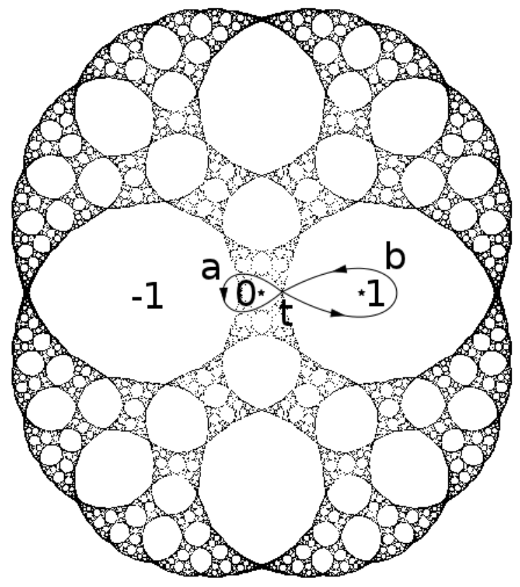
Consider the quadratic polynomial Q−1:z↦z2−1Q_{-1}:z\mapsto z^{2}-1 whose Julia set, called Basilica, is shown in Figure 3. Its critical point 0 is periodic of period 2.

−1\textstyle{-1\ignorespaces\ignorespaces\ignorespaces\ignorespaces\ignorespaces}1:1\scriptstyle{1:1}0\textstyle{0\ignorespaces\ignorespaces\ignorespaces\ignorespaces\ignorespaces}2:1\scriptstyle{2:1}

That induces a degree 2 partial self-covering Q−1:ℂ\{−1,0,1}→ℂ\{−1,0}Q_{-1}:\mathbb{C}\backslash\{-1,0,1\}\rightarrow\mathbb{C}\backslash\{-1,0\}.

Refer to caption
Figure 3: The Basilica and two generators of π1​(ℂ\{−1,0},t)\pi_{1}(\mathbb{C}\backslash\{-1,0\},t)

Choose the fixed point t=1−52t=\frac{1-\sqrt{5}}{2} as base point. The fundamental group π1​(ℂ\{−1,0},t)\pi_{1}(\mathbb{C}\backslash\{-1,0\},t) may be described as the free group generated by two homotopy classes [a],[b][a],[b] where the loop aa surrounds the post-critical point −1-1 and the loop bb the post-critical point 00 both in a counterclockwise motion (see Figure 3).

Refer to caption
Figure 4: The labeling choice ℓ0,ℓ1\ell_{0},\ell_{1} and the lifts of a,ba,b

Let x0=t,x1=−tx_{0}=t,x_{1}=-t be the preimages of tt and choose two paths ℓ0,ℓ1\ell_{0},\ell_{1} from tt to x0,x1x_{0},x_{1} as it is shown in Figure 4. This picture also depicts the lifts of the loops aa and bb. In particular, one can deduce the monodromy action of [a][a] and [b][b] on the first level.

{[a]​0=1[a]​1=0and{[b]​0=0[b]​1=1\left\{\begin{array}[]{l}[a]0=1\\ {[a]}1=0\end{array}\right.\quad\text{and}\quad\left\{\begin{array}[]{l}[b]0=0\\ {[b]}1=1\end{array}\right.

Furthermore

{[ℓ0.A0.ℓ1−1]=[b][ℓ1.A1.ℓ0−1]=[1t]and{[ℓ0.B0.ℓ0−1]=[a][ℓ1.B1.ℓ1−1]=[1t]\left\{\begin{array}[]{l}[\ell_{0}.A_{0}.\ell_{1}^{-1}]=[b]\\ {[\ell_{1}.A_{1}.\ell_{0}^{-1}]}=[1_{t}]\end{array}\right.\quad\text{and}\quad\left\{\begin{array}[]{l}[\ell_{0}.B_{0}.\ell_{0}^{-1}]=[a]\\ {[\ell_{1}.B_{1}.\ell_{1}^{-1}]}=[1_{t}]\end{array}\right.

where [1t][1_{t}] is the homotopy class of the constant loop at base point tt (that is the identity element of the fundamental group π1​(ℂ\{−1,0},t)\pi_{1}(\mathbb{C}\backslash\{-1,0\},t)). It follows from Lemma 3.1 that

∀w∈ℰ⋆,{[a]​0​w=1​([b]​w)[a]​1​w=0​wand{[b]​0​w=0​([a]​w)[b]​1​w=1​w\forall w\in\mathcal{E}^{\star},\quad\left\{\begin{array}[]{l}[a]0w=1([b]w)\\ {[a]}1w=0w\end{array}\right.\quad\text{and}\quad\left\{\begin{array}[]{l}[b]0w=0([a]w)\\ {[b]}1w=1w\end{array}\right.

Therefore the iterated monodromy group of Q−1Q_{-1} seen as a subgroup of Aut⁡(T2)\Aut(T_{2}) is generated by the following wreath recursions

IMG⁡(Q−1,t)=⟨a=(0,1)​⟨⟨b,Id⟩⟩,b=⟨⟨a,Id⟩⟩⟩\IMG(Q_{-1},t)=\Big\langle a=(0,1){\langle\!\langle}b,\Id{\rangle\!\rangle},b={\langle\!\langle}a,\Id{\rangle\!\rangle}\Big\rangle

This group is called the Basilica group. It is not isomorphic to the free group on a set of two elements. Indeed it follows from Lemma 1.1 that

a=(0,1)​⟨⟨b,Id⟩⟩a=(0,1){\langle\!\langle}b,\Id{\rangle\!\rangle} b=⟨⟨a,Id⟩⟩b={\langle\!\langle}a,\Id{\rangle\!\rangle} a−1=(0,1)​⟨⟨Id,b−1⟩⟩a^{-1}=(0,1){\langle\!\langle}\Id,b^{-1}{\rangle\!\rangle} b−1=⟨⟨a−1,Id⟩⟩b^{-1}={\langle\!\langle}a^{-1},\Id{\rangle\!\rangle}
0\textstyle{0\ignorespaces\ignorespaces\ignorespaces\ignorespaces}b\scriptstyle{\textstyle b}0\textstyle{0}1\textstyle{1\ignorespaces\ignorespaces\ignorespaces\ignorespaces}1\textstyle{1} 0\textstyle{0\ignorespaces\ignorespaces\ignorespaces\ignorespaces}a\scriptstyle{\textstyle a}0\textstyle{0}1\textstyle{1\ignorespaces\ignorespaces\ignorespaces\ignorespaces}1\textstyle{1} 0\textstyle{0\ignorespaces\ignorespaces\ignorespaces\ignorespaces}0\textstyle{0}1\textstyle{1\ignorespaces\ignorespaces\ignorespaces\ignorespaces}b−1\scriptstyle{\textstyle b^{-1}}1\textstyle{1} 0\textstyle{0\ignorespaces\ignorespaces\ignorespaces\ignorespaces}a−1\scriptstyle{\textstyle a^{-1}}0\textstyle{0}1\textstyle{1\ignorespaces\ignorespaces\ignorespaces\ignorespaces}1\textstyle{1}

And thus the monodromy action of [b−1.a−1.b−1.a.b.a−1.b.a][b^{-1}.a^{-1}.b^{-1}.a.b.a^{-1}.b.a] is given by the following wreath recursion

0\textstyle{0\ignorespaces\ignorespaces\ignorespaces\ignorespaces}a−1\scriptstyle{\textstyle a^{-1}}0\textstyle{0\ignorespaces\ignorespaces\ignorespaces\ignorespaces}0\textstyle{0\ignorespaces\ignorespaces\ignorespaces\ignorespaces}a−1\scriptstyle{\textstyle a^{-1}}0\textstyle{0\ignorespaces\ignorespaces\ignorespaces\ignorespaces}b\scriptstyle{\textstyle b}0\textstyle{0\ignorespaces\ignorespaces\ignorespaces\ignorespaces}a\scriptstyle{\textstyle a}0\textstyle{0\ignorespaces\ignorespaces\ignorespaces\ignorespaces}0\textstyle{0\ignorespaces\ignorespaces\ignorespaces\ignorespaces}a\scriptstyle{\textstyle a}0\textstyle{0\ignorespaces\ignorespaces\ignorespaces\ignorespaces}b\scriptstyle{\textstyle b}0\textstyle{0}1\textstyle{1\ignorespaces\ignorespaces\ignorespaces\ignorespaces}1\textstyle{1\ignorespaces\ignorespaces\ignorespaces\ignorespaces}b−1\scriptstyle{\textstyle b^{-1}}1\textstyle{1\ignorespaces\ignorespaces\ignorespaces\ignorespaces}1\textstyle{1\ignorespaces\ignorespaces\ignorespaces\ignorespaces}1\textstyle{1\ignorespaces\ignorespaces\ignorespaces\ignorespaces}1\textstyle{1\ignorespaces\ignorespaces\ignorespaces\ignorespaces}b−1\scriptstyle{\textstyle b^{-1}}1\textstyle{1\ignorespaces\ignorespaces\ignorespaces\ignorespaces}1\textstyle{1\ignorespaces\ignorespaces\ignorespaces\ignorespaces}1\textstyle{1}

that is after “untying” (see Lemma 1.1)

0\textstyle{0\ignorespaces\ignorespaces\ignorespaces\ignorespaces}a−1.a=Id\scriptstyle{\textstyle a^{-1}.a=\Id}0\textstyle{0}1\textstyle{1\ignorespaces\ignorespaces\ignorespaces\ignorespaces}b−1.a−1.b.b−1.a.b=Id\scriptstyle{\textstyle b^{-1}.a^{-1}.b.b^{-1}.a.b=\Id}1\textstyle{1}

Therefore [b−1.a−1.b−1.a.b.a−1.b.a]∈Ker(Φ)[b^{-1}.a^{-1}.b^{-1}.a.b.a^{-1}.b.a]\in\Ker(\Phi). In particular for every pair of generators of IMG⁡(Q−1,t)\IMG(Q_{-1},t), the relation b−1.a−1.b−1.a.b.a−1.b.a=Idb^{-1}.a^{-1}.b^{-1}.a.b.a^{-1}.b.a=\Id implies a relation between these generators. It follows that IMG⁡(Q−1,t)\IMG(Q_{-1},t) is not isomorphic to the free group on a set of two elements.

Notice that the monodromy action of Q−1:ℂ\{−1,0,1}→ℂ\{−1,0}Q_{-1}:\mathbb{C}\backslash\{-1,0,1\}\rightarrow\mathbb{C}\backslash\{-1,0\} is not faithful. More precisely this group was studied in [GŻ02] where it was in particular proved that

Ker(Φ)=⟨[b−p.a−p.b−p.ap.bp.a−p.bp.ap],[a−2​p.b−p.a−2​p.bp.a2​p.b−p.a2​p.bp]/p=2j,j⩾0⟩\Ker(\Phi)=\Big\langle[b^{-p}.a^{-p}.b^{-p}.a^{p}.b^{p}.a^{-p}.b^{p}.a^{p}],[a^{-2p}.b^{-p}.a^{-2p}.b^{p}.a^{2p}.b^{-p}.a^{2p}.b^{p}]\ /\ p=2^{j},j\geqslant 0\Big\rangle

Chebyshev polynomials and infinite dihedral group

Consider the degree d⩾2d\geqslant 2 Chebyshev polynomials defined by Cd:z↦cos⁡(d​arccos⁡(z))C_{d}:z\mapsto\cos(d\arccos(z)) or equivalently by the following recursive formula

∀z∈ℂ,C0​(z)=1,C1​(z)=z​ and ​Cd​(z)=2​z​Cd−1​(z)−Cd−2​(z)\forall z\in\mathbb{C},\quad C_{0}(z)=1,\ C_{1}(z)=z\text{ and }C_{d}(z)=2zC_{d-1}(z)-C_{d-2}(z)

Its Julia set is the real segment [−2,2][-2,2]. For every k∈{1,2,…,d−1}k\in\{1,2,\dots,d-1\}, the point ck=c​o​s​(π​kd)c_{k}=cos(\frac{\pi k}{d}) is a simple critical point and is mapped to Cd​(ck)=(−1)kC_{d}(c_{k})=(-1)^{k}. Moreover Cd​(1)=1C_{d}(1)=1, Cd​(−1)=(−1)dC_{d}(-1)=(-1)^{d}, and thus the post-critical set is {−1,1}\{-1,1\}. It follows that every Chebyshev polynomial induces a partial self-covering Cd:ℂ\Cd−1​({−1,1})⟶ℂ\{−1,1}C_{d}:\mathbb{C}\backslash C_{d}^{-1}(\{-1,1\})\longrightarrow\mathbb{C}\backslash\{-1,1\}.

Choose t=0t=0 as base point. The fundamental group π1​(ℂ\{−1,1},t)\pi_{1}(\mathbb{C}\backslash\{-1,1\},t) may be described as the free group generated by two homotopy classes [a],[b][a],[b] where the loop aa surrounds the post-critical point −1-1 and the loop bb the post-critical point 11 both in a counterclockwise motion (see the graph below).

−1\textstyle{-1}t\textstyle{t\ignorespaces\ignorespaces\ignorespaces\ignorespaces\ignorespaces\ignorespaces\ignorespaces\ignorespaces\ignorespaces\ignorespaces\ignorespaces\ignorespaces\ignorespaces\ignorespaces}a\scriptstyle{\textstyle a}b\scriptstyle{\textstyle b}1\textstyle{1}

The preimages of t=0t=0 are xε=cos⁡(π2​d+π​εd)x_{\varepsilon}=\cos(\frac{\pi}{2d}+\frac{\pi\varepsilon}{d}) where the letter ε\varepsilon belongs to the alphabet ℰ={0,1,…,d−1}\mathcal{E}=\{0,1,\dots,d-1\}. For every letter ε∈ℰ\varepsilon\in\mathcal{E}, let ℓε\ell_{\varepsilon} be the straight path from tt to xεx_{\varepsilon}. Remark that every real segment [xk+1,xk][x_{k+1},x_{k}] contains only one critical point, namely ck+1c_{k+1}, and the restriction of CdC_{d} on this segment is a double covering map onto [−1,0][-1,0] for kk even and onto [0,1][0,1] for kk odd.

Each of the loops aa and bb has exactly dd lifts. The pattern of these lifts is depicted in the following graph

…\textstyle{\dots}x4\textstyle{x_{4}\ignorespaces\ignorespaces\ignorespaces\ignorespaces\ignorespaces}B4\scriptstyle{\textstyle B_{4}}c4\textstyle{c_{4}}x3\textstyle{x_{3}\ignorespaces\ignorespaces\ignorespaces\ignorespaces\ignorespaces\ignorespaces\ignorespaces\ignorespaces\ignorespaces\ignorespaces}B3\scriptstyle{\textstyle B_{3}}A3\scriptstyle{\textstyle A_{3}}c3\textstyle{c_{3}}x2\textstyle{x_{2}\ignorespaces\ignorespaces\ignorespaces\ignorespaces\ignorespaces\ignorespaces\ignorespaces\ignorespaces\ignorespaces\ignorespaces}B2\scriptstyle{\textstyle B_{2}}A2\scriptstyle{\textstyle A_{2}}c2\textstyle{c_{2}}x1\textstyle{x_{1}\ignorespaces\ignorespaces\ignorespaces\ignorespaces\ignorespaces\ignorespaces\ignorespaces\ignorespaces\ignorespaces\ignorespaces}B1\scriptstyle{\textstyle B_{1}}A1\scriptstyle{\textstyle A_{1}}c1\textstyle{c_{1}}x0\textstyle{x_{0}\ignorespaces\ignorespaces\ignorespaces\ignorespaces\ignorespaces\ignorespaces\ignorespaces\ignorespaces\ignorespaces\ignorespaces\ignorespaces\ignorespaces}B0\scriptstyle{\textstyle B_{0}}A0\scriptstyle{\textstyle A_{0}}1\textstyle{1}

and the last lift on left, which is a loop surrounding −1-1, is a lift of bb for dd even and of aa for dd odd. It follows from Lemma 3.1 that

∀w∈ℰ⋆,{[a]​0​w=1​w[a]​1​w=0​w[a]​2​w=3​w[a]​3​w=2​w…and{[b]​0​w=0​([b]​w)[b]​1​w=2​w[b]​2​w=1​w[b]​3​w=4​w[b]​4​w=3​w…\forall w\in\mathcal{E}^{\star},\quad\left\{\begin{array}[]{l}[a]0w=1w\\ {[a]}1w=0w\\ {[a]}2w=3w\\ {[a]}3w=2w\\ \dots\end{array}\right.\quad\text{and}\quad\left\{\begin{array}[]{l}[b]0w=0([b]w)\\ {[b]}1w=2w\\ {[b]}2w=1w\\ {[b]}3w=4w\\ {[b]}4w=3w\\ \dots\end{array}\right.
with{[b]​(d−1)​w=(d−1)​([a]​w)if ​d​ is even[a]​(d−1)​w=(d−1)​([a]​w)if ​d​ is odd\text{with}\quad\left\{\begin{array}[]{cc}{[b]}(d-1)w=(d-1)([a]w)&\text{if }d\text{ is even}\\ {[a]}(d-1)w=(d-1)([a]w)&\text{if }d\text{ is odd}\end{array}\right.

That leads to the following wreath recursions

{a=σa​⟨⟨Id,Id,…,Id,Id⟩⟩andb=σb​⟨⟨b,Id,…,Id,a⟩⟩if ​d​ is evena=σa​⟨⟨Id,Id,…,Id,a⟩⟩andb=σb​⟨⟨b,Id,…,Id,Id⟩⟩if ​d​ is odd\left\{\begin{array}[]{cccc}a=\sigma_{a}{\langle\!\langle}\Id,\Id,\dots,\Id,\Id{\rangle\!\rangle}&\text{and}&b=\sigma_{b}{\langle\!\langle}b,\Id,\dots,\Id,a{\rangle\!\rangle}&\text{if }d\text{ is even}\\ a=\sigma_{a}{\langle\!\langle}\Id,\Id,\dots,\Id,a{\rangle\!\rangle}&\text{and}&b=\sigma_{b}{\langle\!\langle}b,\Id,\dots,\Id,\Id{\rangle\!\rangle}&\text{if }d\text{ is odd}\end{array}\right.
whereσa=(0,1)​(2,3)​…andσb=(1,2)​(3,4)​…\text{where}\quad\sigma_{a}=(0,1)(2,3)\dots\quad\text{and}\quad\sigma_{b}=(1,2)(3,4)\dots

Using Lemma 1.1, one may compute the wreath recursions a2a^{2} and b2b^{2}.

{a2=⟨⟨Id,Id,…,Id,Id⟩⟩andb2=⟨⟨b2,Id,…,Id,a2⟩⟩if ​d​ is evena2=⟨⟨Id,Id,…,Id,a2⟩⟩andb=⟨⟨b2,Id,…,Id,Id⟩⟩if ​d​ is odd\left\{\begin{array}[]{cccc}a^{2}={\langle\!\langle}\Id,\Id,\dots,\Id,\Id{\rangle\!\rangle}&\text{and}&b^{2}={\langle\!\langle}b^{2},\Id,\dots,\Id,a^{2}{\rangle\!\rangle}&\text{if }d\text{ is even}\\ a^{2}={\langle\!\langle}\Id,\Id,\dots,\Id,a^{2}{\rangle\!\rangle}&\text{and}&b={\langle\!\langle}b^{2},\Id,\dots,\Id,\Id{\rangle\!\rangle}&\text{if }d\text{ is odd}\end{array}\right.

Applying Lemma 1.1, it follows that a2=b2=Ida^{2}=b^{2}=\Id, or equivalently, in terms of monodromy action,

⟨[a2],[b2]⟩⊂K​e​r​(Φ)⊂⟨[a],[b]⟩=π1​(ℂ\{−1,1},t)\Big\langle[a^{2}],[b^{2}]\Big\rangle\subset Ker(\Phi)\subset\Big\langle[a],[b]\Big\rangle=\pi_{1}(\mathbb{C}\backslash\{-1,1\},t)

Remark that if Ker⁡(Φ)\Ker(\Phi) is strictly larger than ⟨[a2],[b2]⟩\langle[a^{2}],[b^{2}]\rangle, then Ker⁡(Φ)\Ker(\Phi) must contain at least one element of the form either [(a.b)j][(a.b)^{j}] or [(b.a)j][(b.a)^{j}] with j⩾1j\geqslant 1 or of the form either [a.(b.a)j][a.(b.a)^{j}] or [b.(a.b)j][b.(a.b)^{j}] with j⩾0j\geqslant 0. One will prove that is not the case.

The wreath recursion a.ba.b is given by (using Lemma 1.1)

{a.b=σa.b​⟨⟨Id,b,Id,…,Id,a,Id⟩⟩if ​d​ is evena.b=σa.b​⟨⟨Id,b,Id,…,Id,Id,a⟩⟩if ​d​ is odd\left\{\begin{array}[]{cc}a.b=\sigma_{a.b}{\langle\!\langle}\Id,b,\Id,\dots,\Id,a,\Id{\rangle\!\rangle}&\text{if }d\text{ is even}\\ a.b=\sigma_{a.b}{\langle\!\langle}\Id,b,\Id,\dots,\Id,\Id,a{\rangle\!\rangle}&\text{if }d\text{ is odd}\end{array}\right.

where (using circular notation)

σa.b\displaystyle\sigma_{a.b} =\displaystyle= ((1,2)​(3,4)​…)∘((0,1)​(2,3)​…)\displaystyle\Big((1,2)(3,4)\dots\Big)\circ\Big((0,1)(2,3)\dots\Big)
=\displaystyle= {(0,2,4,…,d−4,d−2,d−1,d−3,…,5,3,1)if ​d​ is even(0,2,4,…,d−3,d−1,d−2,d−4,…,5,3,1)if ​d​ is odd\displaystyle\left\{\begin{array}[]{cc}(0,2,4,\dots,d-4,d-2,d-1,d-3,\dots,5,3,1)&\text{if }d\text{ is even}\\ (0,2,4,\dots,d-3,d-1,d-2,d-4,\dots,5,3,1)&\text{if }d\text{ is odd}\end{array}\right.

In particular [a.b][a.b] acts as a cyclic permutation of order dd on the first level of the regular rooted tree TdT_{d} (since σa.b\sigma_{a.b} is of order dd). Moreover, using Lemma 1.1 again, it appears that

(a.b)d=⟨⟨a.b,a.b,a.b,…,b.a,b.a,b.a⟩⟩(a.b)^{d}={\langle\!\langle}a.b,a.b,a.b,\dots,b.a,b.a,b.a{\rangle\!\rangle}

Recall that (b.a)=(a.b)−1(b.a)=(a.b)^{-1} since a2=b2=Ida^{2}=b^{2}=\Id, and thus [b.a][b.a] also acts as a cyclic permutation of order dd on the first level. Therefore a quick induction implies that [a.b][a.b] and [b.a][b.a] act as a cyclic permutation of order dnd^{n} on the nn-th level of TdT_{d}. It follows that none of the elements of the form either [(a.b)j][(a.b)^{j}] or [(b.a)j][(b.a)^{j}] with j⩾1j\geqslant 1 acts as the identity tree automorphism. The same holds as well for the elements of the form either [a.(b.a)j][a.(b.a)^{j}] or [b.(a.b)j][b.(a.b)^{j}] with j⩾0j\geqslant 0 since aa and bb are of order 2 in Aut⁡(Td)\Aut(T_{d}). Finally

Ker⁡(Φ)=⟨[a2],[b2]⟩andIMG⁡(Cd,t)=π1​(ℂ\{−1,1},t)/Ker⁡(Φ)=⟨[a],[b]⟩/⟨[a2],[b2]⟩\Ker(\Phi)=\Big\langle[a^{2}],[b^{2}]\Big\rangle\quad\text{and}\quad\IMG(C_{d},t)=\pi_{1}(\mathbb{C}\backslash\{-1,1\},t)/\Ker(\Phi)=\Big\langle[a],[b]\Big\rangle/\Big\langle[a^{2}],[b^{2}]\Big\rangle

This group is called the infinite dihedral group. It is isomorphic to the isometry group of ℤ\mathbb{Z} (for instance the permutations α↦−α\alpha\mapsto-\alpha and α↦1−α\alpha\mapsto 1-\alpha play the same role as aa and bb).

The quadratic rational map z↦(z−1z+1)2z\mapsto\left(\frac{z-1}{z+1}\right)^{2}

Consider the quadratic rational map R:z↦(z−1z+1)2R:z\mapsto\left(\frac{z-1}{z+1}\right)^{2} whose Julia set is shown in Figure 5. The critical points are −1-1 and 11. Since R⁡(−1)=∞R(-1)=\infty, R2​(−1)=1R^{2}(-1)=1 and R⁡(1)=0R(1)=0, R2​(1)=1R^{2}(1)=1, the post-critical set is {0,1,∞}\{0,1,\infty\}.

−1\textstyle{-1\ignorespaces\ignorespaces\ignorespaces\ignorespaces\ignorespaces}2:1\scriptstyle{2:1}0\textstyle{0\ignorespaces\ignorespaces\ignorespaces\ignorespaces\ignorespaces}1:1\scriptstyle{1:1}1\textstyle{1\ignorespaces\ignorespaces\ignorespaces\ignorespaces\ignorespaces}2:1\scriptstyle{2:1}∞\textstyle{\infty\ignorespaces\ignorespaces\ignorespaces\ignorespaces\ignorespaces}1:1\scriptstyle{1:1}

That induces a degree 2 partial self-covering R:ℂ\{−1,0,1}⟶ℂ\{0,1}R:\mathbb{C}\backslash\{-1,0,1\}\longrightarrow\mathbb{C}\backslash\{0,1\}.

Refer to caption
Figure 5: The Julia set of R:z↦(z−1z+1)2R:z\mapsto\left(\frac{z-1}{z+1}\right)^{2} and two generators of π1​(ℂ\{0,1},t)\pi_{1}(\mathbb{C}\backslash\{0,1\},t)

Choose the real fixed point t≈0.296t\approx 0.296 as base point. The fundamental group π1​(ℂ\{0,1},t)\pi_{1}(\mathbb{C}\backslash\{0,1\},t) may be described as the free group generated by two homotopy classes [a],[b][a],[b] where the loop aa surrounds the post-critical point 0 and the loop bb the post-critical point 1 both in a counterclockwise motion (see Figure 5).
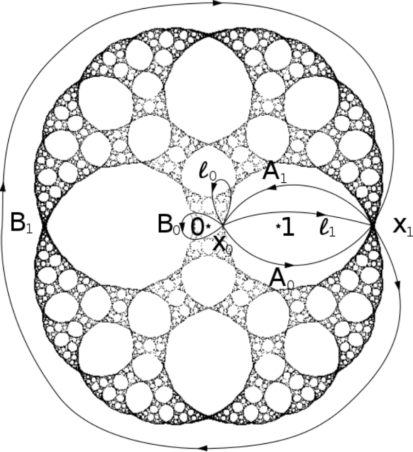
Refer to caption
Figure 6: The labeling choice ℓ0,ℓ1\ell_{0},\ell_{1} and the lifts of a,ba,b

Let x0=t,x1=t−1≈3.383x_{0}=t,x_{1}=t^{-1}\approx 3.383 be the preimages of tt and choose two paths ℓ0,ℓ1\ell_{0},\ell_{1} from tt to x0,x1x_{0},x_{1} as it is shown in Figure 6. This picture also depicts the lifts of the loops aa and bb. By using Lemma 3.1, one can compute the monodromy action of [a][a] and [b][b].

∀w∈ℰ⋆,{[a]​0​w=1​([b]​w)[a]​1​w=0​wand{[b]​0​w=0​([a]​w)[b]1w=1([b−1.a−1]w)\forall w\in\mathcal{E}^{\star},\quad\left\{\begin{array}[]{l}[a]0w=1([b]w)\\ {[a]}1w=0w\end{array}\right.\quad\text{and}\quad\left\{\begin{array}[]{l}[b]0w=0([a]w)\\ {[b]}1w=1([b^{-1}.a^{-1}]w)\end{array}\right.

Therefore the iterated monodromy group of RR seen as a subgroup of Aut⁡(T2)\Aut(T_{2}) is generated by the following wreath recursions

IMG(R,t)=⟨a=(0,1)⟨⟨b,Id⟩⟩,b=⟨⟨a,b−1.a−1⟩⟩⟩\IMG(R,t)=\Big\langle a=(0,1){\langle\!\langle}b,\Id{\rangle\!\rangle},b={\langle\!\langle}a,b^{-1}.a^{-1}{\rangle\!\rangle}\Big\rangle

Notice that these wreath recursions are not convenient to compute with since two generators occur in the renormalization ℛ1​(b)=b−1.a−1\mathcal{R}_{1}(b)=b^{-1}.a^{-1} and only one renormalization is the identity tree automorphism. However one may find a nicer pair of generators of IMG⁡(R,t)\IMG(R,t) by taking another pair of generators of π1​(ℂ\{0,1},t)\pi_{1}(\mathbb{C}\backslash\{0,1\},t) and another labeling choice.

Indeed consider the tree automorphism gg in Aut⁡(T2)\Aut(T_{2}) whose wreath recursion is given by

g=⟨⟨g.a,g⟩⟩g={\langle\!\langle}g.a,g{\rangle\!\rangle}

This tree automorphism is well defined by induction on the successive levels of the regular rooted tree T2T_{2}. Now consider the following wreath recursions

a′a^{\prime} = g.(a.b).g−1g.(a.b).g^{-1} = 0\textstyle{0\ignorespaces\ignorespaces\ignorespaces\ignorespaces}g.a\scriptstyle{\textstyle g.a}0\textstyle{0\ignorespaces\ignorespaces\ignorespaces\ignorespaces}b\scriptstyle{\textstyle b}0\textstyle{0\ignorespaces\ignorespaces\ignorespaces\ignorespaces}a\scriptstyle{\textstyle a}0\textstyle{0\ignorespaces\ignorespaces\ignorespaces\ignorespaces}a−1.g−1\scriptstyle{\textstyle a^{-1}.g^{-1}}0\textstyle{0}1\textstyle{1\ignorespaces\ignorespaces\ignorespaces\ignorespaces}g\scriptstyle{\textstyle g}1\textstyle{1\ignorespaces\ignorespaces\ignorespaces\ignorespaces}1\textstyle{1\ignorespaces\ignorespaces\ignorespaces\ignorespaces}b−1.a−1\scriptstyle{\textstyle b^{-1}.a^{-1}}1\textstyle{1\ignorespaces\ignorespaces\ignorespaces\ignorespaces}g−1\scriptstyle{\textstyle g^{-1}}1\textstyle{1}
= 0\textstyle{0\ignorespaces\ignorespaces\ignorespaces\ignorespaces}g.a.b.b−1.a−1.g−1=Id\scriptstyle{\textstyle\quad g.a.b.b^{-1}.a^{-1}.g^{-1}=\Id}0\textstyle{0}1\textstyle{1\ignorespaces\ignorespaces\ignorespaces\ignorespaces}g.a.a−1.g−1=Id\scriptstyle{\textstyle\quad g.a.a^{-1}.g^{-1}=\Id}1\textstyle{1} = (0,1)​⟨⟨Id,Id⟩⟩(0,1){\langle\!\langle}\Id,\Id{\rangle\!\rangle}
b′b^{\prime} = g.a.g−1g.a.g^{-1} = 0\textstyle{0\ignorespaces\ignorespaces\ignorespaces\ignorespaces}g.a\scriptstyle{\textstyle g.a}0\textstyle{0\ignorespaces\ignorespaces\ignorespaces\ignorespaces}b\scriptstyle{\textstyle b}0\textstyle{0\ignorespaces\ignorespaces\ignorespaces\ignorespaces}a−1.g−1\scriptstyle{\textstyle a^{-1}.g^{-1}}0\textstyle{0}1\textstyle{1\ignorespaces\ignorespaces\ignorespaces\ignorespaces}g\scriptstyle{\textstyle g}1\textstyle{1\ignorespaces\ignorespaces\ignorespaces\ignorespaces}1\textstyle{1\ignorespaces\ignorespaces\ignorespaces\ignorespaces}g−1\scriptstyle{\textstyle g^{-1}}1\textstyle{1}
= 0\textstyle{0\ignorespaces\ignorespaces\ignorespaces\ignorespaces}g.a.b.g−1=a′\scriptstyle{\textstyle\quad g.a.b.g^{-1}=a^{\prime}}0\textstyle{0}1\textstyle{1\ignorespaces\ignorespaces\ignorespaces\ignorespaces}g.a−1.g−1=b′−1\scriptstyle{\textstyle\quad g.a^{-1}.g^{-1}=b^{\prime-1}}1\textstyle{1} = (0,1)​⟨⟨a′,b′−1⟩⟩(0,1){\langle\!\langle}a^{\prime},b^{\prime-1}{\rangle\!\rangle}

Remark that ⟨a,b⟩\langle a,b\rangle is obviously generated by a.ba.b and aa. Consequently ⟨a,b⟩\langle a,b\rangle and ⟨a′,b′⟩=g.⟨a.b,a⟩.g−1=g.⟨a,b⟩.g−1\langle a^{\prime},b^{\prime}\rangle=g.\langle a.b,a\rangle.g^{-1}=g.\langle a,b\rangle.g^{-1} are conjugate subgroups in Aut⁡(T2)\Aut(T_{2})

Recall that the iterated monodromy group IMG⁡(R,t)\IMG(R,t) seen as a subgroup of Aut⁡(T2)\Aut(T_{2}) is defined for a given labeling choice. In particular the subgroup ⟨a,b⟩\langle a,b\rangle was obtained for the labeling choice, say (L)(L), depicted in Figure 6. With similar computations, one can show that the labeling choice (L′)(L^{\prime}) depicted in Figure 7 gives the subgroup ⟨a′,b′⟩\langle a^{\prime},b^{\prime}\rangle. In other words, the tree automorphism g∈Aut⁡(T2)g\in\Aut(T_{2}) corresponds to the map φ(L),(L′)=φ(L)∘(φ(L′))−1∈Aut⁡(T2)\varphi^{(L),(L^{\prime})}=\varphi^{(L)}\circ\left(\varphi^{(L^{\prime})}\right)^{-1}\in\Aut(T_{2}) which describes the change of labeling choices from (L)(L) to (L′)(L^{\prime}) (see Proposition 2.2 and Definition 3.1).
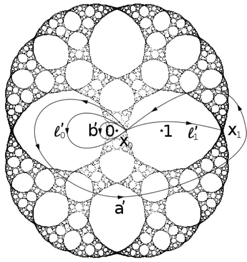
Refer to caption
Figure 7: The labeling choice ℓ0′,ℓ1′\ell^{\prime}_{0},\ell^{\prime}_{1} and two generators [a′]=[a.b],[b′]=[a][a^{\prime}]=[a.b],[b^{\prime}]=[a] of π1​(ℂ\{0,1},t)\pi_{1}(\mathbb{C}\backslash\{0,1\},t)

It follows from the labeling choice (L′)(L^{\prime}) that

IMG⁡(R,t)=⟨a′=(0,1)​⟨⟨Id,Id⟩⟩,b′=(0,1)​⟨⟨a′,b′−1⟩⟩⟩\IMG(R,t)=\Big\langle a^{\prime}=(0,1){\langle\!\langle}\Id,\Id{\rangle\!\rangle},b^{\prime}=(0,1){\langle\!\langle}a^{\prime},b^{\prime-1}{\rangle\!\rangle}\Big\rangle

for which the wreath recursions of generators are nicer than for ⟨a,b⟩\langle a,b\rangle. Indeed, that immediately shows a′2=Ida^{\prime 2}=\Id, and thus IMG⁡(R,t)\IMG(R,t) is not isomorphic to the free group on a set of two elements, or equivalently the monodromy action of R:ℂ\{−1,0,1}→ℂ\{0,1}R:\mathbb{C}\backslash\{-1,0,1\}\rightarrow\mathbb{C}\backslash\{0,1\} is not faithful.

Sierpinski gasket and towers of Hanoi (due to Grigorchuk and S̆unić [GŠ07])

Consider the cubic rational map H:z↦z2−1627​zH:z\mapsto z^{2}-\frac{16}{27z} whose Julia set is a Sierpinski gasket (see Figure 8). The critical points are ∞\infty and ck=−23​ζkc_{k}=-\frac{2}{3}\zeta^{k} where k∈{0,1,2}k\in\{0,1,2\} and ζ=−12+32\zeta=-\frac{1}{2}+\frac{\sqrt{3}}{2} (a third root of unity). Since H⁡(∞)=∞H(\infty)=\infty and H⁡(ck)=43​ζ2​kH(c_{k})=\frac{4}{3}\zeta^{2k}, H2​(ck)=43​ζkH^{2}(c_{k})=\frac{4}{3}\zeta^{k}, the post-critical set is {43,43​ζ,43​ζ2,∞}\left\{\frac{4}{3},\frac{4}{3}\zeta,\frac{4}{3}\zeta^{2},\infty\right\}.

43​ζ\textstyle{\frac{4}{3}\zeta\ignorespaces\ignorespaces\ignorespaces\ignorespaces\ignorespaces}1:1\scriptstyle{1:1}−23​ζ2\textstyle{-\frac{2}{3}\zeta^{2}\ignorespaces\ignorespaces\ignorespaces\ignorespaces}2:1\scriptstyle{2:1}∞\textstyle{\infty\ignorespaces\ignorespaces\ignorespaces\ignorespaces\ignorespaces\ignorespaces}2:1\scriptstyle{2:1}−23\textstyle{-\frac{2}{3}\ignorespaces\ignorespaces\ignorespaces\ignorespaces}2:1\scriptstyle{2:1}43\textstyle{\frac{4}{3}\ignorespaces\ignorespaces\ignorespaces\ignorespaces\ignorespaces\ignorespaces}1:1\scriptstyle{1:1}−23​ζ\textstyle{-\frac{2}{3}\zeta\ignorespaces\ignorespaces\ignorespaces\ignorespaces}2:1\scriptstyle{2:1}43​ζ2\textstyle{\frac{4}{3}\zeta^{2}\ignorespaces\ignorespaces\ignorespaces\ignorespaces\ignorespaces}1:1\scriptstyle{1:1}

That induces a degree 33 partial self-covering H:ℂ\H−1​({43,43​ζ,43​ζ2})⟶ℂ\{43,43​ζ,43​ζ2}H:\mathbb{C}\backslash H^{-1}\left(\left\{\frac{4}{3},\frac{4}{3}\zeta,\frac{4}{3}\zeta^{2}\right\}\right)\longrightarrow\mathbb{C}\backslash\left\{\frac{4}{3},\frac{4}{3}\zeta,\frac{4}{3}\zeta^{2}\right\}.

Refer to caption
Figure 8: A Sierpinski gasket and three generators of π1​(ℂ\{43,43​ζ,43​ζ2},t)\pi_{1}(\mathbb{C}\backslash\{\frac{4}{3},\frac{4}{3}\zeta,\frac{4}{3}\zeta^{2}\},t)

Choose t=0t=0 as base point. The fundamental group π1​(ℂ\{43,43​ζ,43​ζ2},t)\pi_{1}(\mathbb{C}\backslash\{\frac{4}{3},\frac{4}{3}\zeta,\frac{4}{3}\zeta^{2}\},t) may be described as the free group generated by three homotopy classes [a],[b],[c][a],[b],[c] where the loops a,b,ca,b,c surround the post-critical points 43,43​ζ,43​ζ2\frac{4}{3},\frac{4}{3}\zeta,\frac{4}{3}\zeta^{2} respectively in a counterclockwise motion (see Figure 8).

The preimages of tt are xε=24/33​ζεx_{\varepsilon}=\frac{2^{4/3}}{3}\zeta^{\varepsilon} where the letter ε\varepsilon belongs to the alphabet ℰ={0,1,2}\mathcal{E}=\{0,1,2\}. For every letter ε∈ℰ\varepsilon\in\mathcal{E}, let ℓε\ell_{\varepsilon} be the straight path (in ℂ\mathbb{C}) from tt to xεx_{\varepsilon} as it is shown in Figure 9. This picture also depicts the lifts of the loops a,b,ca,b,c.

Refer to caption
Figure 9: The labeling choice ℓ0,ℓ1,ℓ2\ell_{0},\ell_{1},\ell_{2} and the lifts of a,b,ca,b,c

One can deduce the monodromy action of [a],[b],[c][a],[b],[c] on the first level.

{[a]​0=0[a]​1=2[a]​2=1and{[b]​0=1[b]​1=0[b]​2=2and{[c]​0=2[c]​1=1[c]​2=0\left\{\begin{array}[]{l}[a]0=0\\ {[a]}1=2\\ {[a]}2=1\end{array}\right.\quad\text{and}\quad\left\{\begin{array}[]{l}[b]0=1\\ {[b]}1=0\\ {[b]}2=2\end{array}\right.\quad\text{and}\quad\left\{\begin{array}[]{l}[c]0=2\\ {[c]}1=1\\ {[c]}2=0\end{array}\right.

Furthermore

{[ℓ0.A0.ℓ0−1]=[a][ℓ1.A1.ℓ2−1]=[1t][ℓ2.A2.ℓ1−1]=[1t]and{[ℓ0.B0.ℓ1−1]=[1t][ℓ1.B1.ℓ0−1]=[1t][ℓ2.B2.ℓ2−1]=[c]and{[ℓ0.C0.ℓ2−1]=[1t][ℓ1.C1.c1−1]=[b][ℓ2.C2.ℓ0−1]=[1t]\left\{\begin{array}[]{l}[\ell_{0}.A_{0}.\ell_{0}^{-1}]=[a]\\ {[\ell_{1}.A_{1}.\ell_{2}^{-1}]}=[1_{t}]\\ {[\ell_{2}.A_{2}.\ell_{1}^{-1}]}=[1_{t}]\end{array}\right.\quad\text{and}\quad\left\{\begin{array}[]{l}[\ell_{0}.B_{0}.\ell_{1}^{-1}]=[1_{t}]\\ {[\ell_{1}.B_{1}.\ell_{0}^{-1}]}=[1_{t}]\\ {[\ell_{2}.B_{2}.\ell_{2}^{-1}]}=[c]\end{array}\right.\quad\text{and}\quad\left\{\begin{array}[]{l}[\ell_{0}.C_{0}.\ell_{2}^{-1}]=[1_{t}]\\ {[\ell_{1}.C_{1}.c_{1}^{-1}]}=[b]\\ {[\ell_{2}.C_{2}.\ell_{0}^{-1}]}=[1_{t}]\end{array}\right.

where [1t][1_{t}] is the homotopy class of the constant loop at base point tt (that is the identity element of the fundamental group π1​(ℂ\{43,43​ζ,43​ζ2},t)\pi_{1}(\mathbb{C}\backslash\{\frac{4}{3},\frac{4}{3}\zeta,\frac{4}{3}\zeta^{2}\},t)). It follows from Lemma 3.1 that

∀w∈ℰ⋆,{[a]​0​w=0​([a]​w)[a]​1​w=2​w[a]​2​w=1​wand{[b]​0​w=1​w[b]​1​w=0​w[b]​2​w=2​([c]​w)and{[c]​0​w=2​w[c]​1​w=1​([b]​w)[c]​2​w=0​w\forall w\in\mathcal{E}^{\star},\quad\left\{\begin{array}[]{l}[a]0w=0([a]w)\\ {[a]}1w=2w\\ {[a]}2w=1w\end{array}\right.\quad\text{and}\quad\left\{\begin{array}[]{l}[b]0w=1w\\ {[b]}1w=0w\\ {[b]}2w=2([c]w)\end{array}\right.\quad\text{and}\quad\left\{\begin{array}[]{l}[c]0w=2w\\ {[c]}1w=1([b]w)\\ {[c]}2w=0w\end{array}\right.

Therefore the iterated monodromy group of HH seen as a subgroup of Aut⁡(T3)\Aut(T_{3}) is generated by the following wreath recursions

IMG⁡(H,t)=⟨a=(1,2)​⟨⟨a,Id,Id⟩⟩,b=(0,1)​⟨⟨Id,Id,c⟩⟩,c=(0,2)​⟨⟨Id,b,Id⟩⟩⟩\IMG(H,t)=\Big\langle a=(1,2){\langle\!\langle}a,\Id,\Id{\rangle\!\rangle},b=(0,1){\langle\!\langle}\Id,\Id,c{\rangle\!\rangle},c=(0,2){\langle\!\langle}\Id,b,\Id{\rangle\!\rangle}\Big\rangle

IMG⁡(H,t)\IMG(H,t) is not isomorphic to the free group on a set of three elements (for instance one can prove that a2=b2=c2=Ida^{2}=b^{2}=c^{2}=\Id by using Lemma 1.1 and Lemma 1.1) or equivalently the monodromy action of H:ℂ\H−1​({43,43​ζ,43​ζ2})→ℂ\{43,43​ζ,43​ζ2}H:\mathbb{C}\backslash H^{-1}\left(\left\{\frac{4}{3},\frac{4}{3}\zeta,\frac{4}{3}\zeta^{2}\right\}\right)\rightarrow\mathbb{C}\backslash\left\{\frac{4}{3},\frac{4}{3}\zeta,\frac{4}{3}\zeta^{2}\right\} is not faithful.

Moreover IMG⁡(H,t)\IMG(H,t) looks like the Hanoi Towers group ℋ\mathcal{H} (see Section 1.1). Indeed consider two tree automorphisms g,hg,h in Aut⁡(T3)\Aut(T_{3}) whose wreath recursions are given by


g=(1,2)​⟨⟨h,h,h⟩⟩andh=⟨⟨g,g,g⟩⟩g=(1,2){\langle\!\langle}h,h,h{\rangle\!\rangle}\quad\text{and}\quad h={\langle\!\langle}g,g,g{\rangle\!\rangle}

This pair of tree automorphisms is well defined by induction on the successive levels of the regular rooted tree T3T_{3}. Now consider the following wreath recursions

a′a^{\prime} = g.a.g−1g.a.g^{-1} = 0\textstyle{0\ignorespaces\ignorespaces\ignorespaces\ignorespaces}h\scriptstyle{\textstyle h}0\textstyle{0\ignorespaces\ignorespaces\ignorespaces\ignorespaces}a\scriptstyle{\textstyle a}0\textstyle{0\ignorespaces\ignorespaces\ignorespaces\ignorespaces}h−1\scriptstyle{\textstyle h^{-1}}0\textstyle{0}1\textstyle{1\ignorespaces\ignorespaces\ignorespaces\ignorespaces}h\scriptstyle{\textstyle h}1\textstyle{1\ignorespaces\ignorespaces\ignorespaces\ignorespaces}1\textstyle{1\ignorespaces\ignorespaces\ignorespaces\ignorespaces}h−1\scriptstyle{\textstyle h^{-1}}1\textstyle{1}2\textstyle{2\ignorespaces\ignorespaces\ignorespaces\ignorespaces}h\scriptstyle{\textstyle h}2\textstyle{2\ignorespaces\ignorespaces\ignorespaces\ignorespaces}2\textstyle{2\ignorespaces\ignorespaces\ignorespaces\ignorespaces}h−1\scriptstyle{\textstyle h^{-1}}2\textstyle{2} = 0\textstyle{0\ignorespaces\ignorespaces\ignorespaces\ignorespaces}h.a.h−1\scriptstyle{\textstyle h.a.h^{-1}}0\textstyle{0}1\textstyle{1\ignorespaces\ignorespaces\ignorespaces\ignorespaces}1\textstyle{1}2\textstyle{2\ignorespaces\ignorespaces\ignorespaces\ignorespaces}2\textstyle{2} = (1,2)⟨⟨h.a.h−1,Id,Id⟩⟩(1,2){\langle\!\langle}h.a.h^{-1},\Id,\Id{\rangle\!\rangle}
b′b^{\prime} = g.c.g−1g.c.g^{-1} = 0\textstyle{0\ignorespaces\ignorespaces\ignorespaces\ignorespaces}h\scriptstyle{\textstyle h}0\textstyle{0\ignorespaces\ignorespaces\ignorespaces\ignorespaces\ignorespaces\ignorespaces}0\textstyle{0\ignorespaces\ignorespaces\ignorespaces\ignorespaces}h−1\scriptstyle{\textstyle h^{-1}}0\textstyle{0}1\textstyle{1\ignorespaces\ignorespaces\ignorespaces\ignorespaces}h\scriptstyle{\textstyle h}1\textstyle{1\ignorespaces\ignorespaces\ignorespaces\ignorespaces}b\scriptstyle{\textstyle b}1\textstyle{1\ignorespaces\ignorespaces\ignorespaces\ignorespaces}h−1\scriptstyle{\textstyle h^{-1}}1\textstyle{1}2\textstyle{2\ignorespaces\ignorespaces\ignorespaces\ignorespaces}h\scriptstyle{\textstyle h}2\textstyle{2\ignorespaces\ignorespaces\ignorespaces\ignorespaces\ignorespaces\ignorespaces}2\textstyle{2\ignorespaces\ignorespaces\ignorespaces\ignorespaces}h−1\scriptstyle{\textstyle h^{-1}}2\textstyle{2} = 0\textstyle{0\ignorespaces\ignorespaces\ignorespaces\ignorespaces}0\textstyle{0}1\textstyle{1\ignorespaces\ignorespaces\ignorespaces\ignorespaces}1\textstyle{1}2\textstyle{2\ignorespaces\ignorespaces\ignorespaces\ignorespaces}h.b.h−1\scriptstyle{\textstyle h.b.h^{-1}}2\textstyle{2} = (0,1)⟨⟨Id,Id,h.b.h−1⟩⟩(0,1){\langle\!\langle}\Id,\Id,h.b.h^{-1}{\rangle\!\rangle}
c′c^{\prime} = g.b.g−1g.b.g^{-1} = 0\textstyle{0\ignorespaces\ignorespaces\ignorespaces\ignorespaces}h\scriptstyle{\textstyle h}0\textstyle{0\ignorespaces\ignorespaces\ignorespaces\ignorespaces}0\textstyle{0\ignorespaces\ignorespaces\ignorespaces\ignorespaces}h−1\scriptstyle{\textstyle h^{-1}}0\textstyle{0}1\textstyle{1\ignorespaces\ignorespaces\ignorespaces\ignorespaces}h\scriptstyle{\textstyle h}1\textstyle{1\ignorespaces\ignorespaces\ignorespaces\ignorespaces}1\textstyle{1\ignorespaces\ignorespaces\ignorespaces\ignorespaces}h−1\scriptstyle{\textstyle h^{-1}}1\textstyle{1}2\textstyle{2\ignorespaces\ignorespaces\ignorespaces\ignorespaces}h\scriptstyle{\textstyle h}2\textstyle{2\ignorespaces\ignorespaces\ignorespaces\ignorespaces}c\scriptstyle{\textstyle c}2\textstyle{2\ignorespaces\ignorespaces\ignorespaces\ignorespaces}h−1\scriptstyle{\textstyle h^{-1}}2\textstyle{2} = 0\textstyle{0\ignorespaces\ignorespaces\ignorespaces\ignorespaces\ignorespaces\ignorespaces}0\textstyle{0}1\textstyle{1\ignorespaces\ignorespaces\ignorespaces\ignorespaces}h.c.h−1\scriptstyle{\textstyle h.c.h^{-1}}1\textstyle{1}2\textstyle{2\ignorespaces\ignorespaces\ignorespaces\ignorespaces\ignorespaces\ignorespaces}2\textstyle{2} = (0,2)⟨⟨Id,h.c.h−1,Id⟩⟩(0,2){\langle\!\langle}\Id,h.c.h^{-1},\Id{\rangle\!\rangle}

with

h.a.h−1h.a.h^{-1} = 0\textstyle{0\ignorespaces\ignorespaces\ignorespaces\ignorespaces}g\scriptstyle{\textstyle g}0\textstyle{0\ignorespaces\ignorespaces\ignorespaces\ignorespaces}a\scriptstyle{\textstyle a}0\textstyle{0\ignorespaces\ignorespaces\ignorespaces\ignorespaces}g−1\scriptstyle{\textstyle g^{-1}}0\textstyle{0}1\textstyle{1\ignorespaces\ignorespaces\ignorespaces\ignorespaces}g\scriptstyle{\textstyle g}1\textstyle{1\ignorespaces\ignorespaces\ignorespaces\ignorespaces}1\textstyle{1\ignorespaces\ignorespaces\ignorespaces\ignorespaces}g−1\scriptstyle{\textstyle g^{-1}}1\textstyle{1}2\textstyle{2\ignorespaces\ignorespaces\ignorespaces\ignorespaces}g\scriptstyle{\textstyle g}2\textstyle{2\ignorespaces\ignorespaces\ignorespaces\ignorespaces}2\textstyle{2\ignorespaces\ignorespaces\ignorespaces\ignorespaces}g−1\scriptstyle{\textstyle g^{-1}}2\textstyle{2} = 0\textstyle{0\ignorespaces\ignorespaces\ignorespaces\ignorespaces}g.a.g−1\scriptstyle{\textstyle g.a.g^{-1}}0\textstyle{0}1\textstyle{1\ignorespaces\ignorespaces\ignorespaces\ignorespaces}1\textstyle{1}2\textstyle{2\ignorespaces\ignorespaces\ignorespaces\ignorespaces}2\textstyle{2} = (1,2)​⟨⟨a′,Id,Id⟩⟩(1,2){\langle\!\langle}a^{\prime},\Id,\Id{\rangle\!\rangle}
h.b.h−1h.b.h^{-1} = 0\textstyle{0\ignorespaces\ignorespaces\ignorespaces\ignorespaces}g\scriptstyle{\textstyle g}0\textstyle{0\ignorespaces\ignorespaces\ignorespaces\ignorespaces}0\textstyle{0\ignorespaces\ignorespaces\ignorespaces\ignorespaces}g−1\scriptstyle{\textstyle g^{-1}}0\textstyle{0}1\textstyle{1\ignorespaces\ignorespaces\ignorespaces\ignorespaces}g\scriptstyle{\textstyle g}1\textstyle{1\ignorespaces\ignorespaces\ignorespaces\ignorespaces}1\textstyle{1\ignorespaces\ignorespaces\ignorespaces\ignorespaces}g−1\scriptstyle{\textstyle g^{-1}}1\textstyle{1}2\textstyle{2\ignorespaces\ignorespaces\ignorespaces\ignorespaces}g\scriptstyle{\textstyle g}2\textstyle{2\ignorespaces\ignorespaces\ignorespaces\ignorespaces}c\scriptstyle{\textstyle c}2\textstyle{2\ignorespaces\ignorespaces\ignorespaces\ignorespaces}g−1\scriptstyle{\textstyle g^{-1}}2\textstyle{2} = 0\textstyle{0\ignorespaces\ignorespaces\ignorespaces\ignorespaces}0\textstyle{0}1\textstyle{1\ignorespaces\ignorespaces\ignorespaces\ignorespaces}1\textstyle{1}2\textstyle{2\ignorespaces\ignorespaces\ignorespaces\ignorespaces}g.c.g−1\scriptstyle{\textstyle g.c.g^{-1}}2\textstyle{2} = (0,1)​⟨⟨Id,Id,b′⟩⟩(0,1){\langle\!\langle}\Id,\Id,b^{\prime}{\rangle\!\rangle}
h.c.h−1h.c.h^{-1} = 0\textstyle{0\ignorespaces\ignorespaces\ignorespaces\ignorespaces}g\scriptstyle{\textstyle g}0\textstyle{0\ignorespaces\ignorespaces\ignorespaces\ignorespaces\ignorespaces\ignorespaces}0\textstyle{0\ignorespaces\ignorespaces\ignorespaces\ignorespaces}g−1\scriptstyle{\textstyle g^{-1}}0\textstyle{0}1\textstyle{1\ignorespaces\ignorespaces\ignorespaces\ignorespaces}g\scriptstyle{\textstyle g}1\textstyle{1\ignorespaces\ignorespaces\ignorespaces\ignorespaces}b\scriptstyle{\textstyle b}1\textstyle{1\ignorespaces\ignorespaces\ignorespaces\ignorespaces}g−1\scriptstyle{\textstyle g^{-1}}1\textstyle{1}2\textstyle{2\ignorespaces\ignorespaces\ignorespaces\ignorespaces}g\scriptstyle{\textstyle g}2\textstyle{2\ignorespaces\ignorespaces\ignorespaces\ignorespaces\ignorespaces\ignorespaces}2\textstyle{2\ignorespaces\ignorespaces\ignorespaces\ignorespaces}g−1\scriptstyle{\textstyle g^{-1}}2\textstyle{2} = 0\textstyle{0\ignorespaces\ignorespaces\ignorespaces\ignorespaces\ignorespaces\ignorespaces}0\textstyle{0}1\textstyle{1\ignorespaces\ignorespaces\ignorespaces\ignorespaces}g.b.g−1\scriptstyle{\textstyle g.b.g^{-1}}1\textstyle{1}2\textstyle{2\ignorespaces\ignorespaces\ignorespaces\ignorespaces\ignorespaces\ignorespaces}2\textstyle{2} = (0,2)​⟨⟨Id,c′,Id⟩⟩(0,2){\langle\!\langle}\Id,c^{\prime},\Id{\rangle\!\rangle}

Therefore a quick induction gives

{a′=(1,2)​⟨⟨a′,Id,Id⟩⟩b′=(0,1)​⟨⟨Id,Id,b′⟩⟩c′=(0,2)​⟨⟨Id,c′,Id⟩⟩\left\{\begin{array}[]{l}a^{\prime}=(1,2){\langle\!\langle}a^{\prime},\Id,\Id{\rangle\!\rangle}\\ b^{\prime}=(0,1){\langle\!\langle}\Id,\Id,b^{\prime}{\rangle\!\rangle}\\ c^{\prime}=(0,2){\langle\!\langle}\Id,c^{\prime},\Id{\rangle\!\rangle}\end{array}\right.

These wreath recursions are the three generators of the Hanoi Towers group ℋ\mathcal{H} (see Section 1.1), and thus g.⟨a,b,c⟩.g−1=ℋg.\langle a,b,c\rangle.g^{-1}=\mathcal{H}. Consequently the iterated monodromy group IMG⁡(H,t)\IMG(H,t) seen as a subgroup of Aut⁡(T3)\Aut(T_{3}) is conjugate to the Hanoi Towers group ℋ\mathcal{H} by a tree automorphism of T3T_{3}.

But one can show that gg does not correspond to a map of the form φ(L),(L′)=φ(L)∘(φ(L′))−1\varphi^{(L),(L^{\prime})}=\varphi^{(L)}\circ\left(\varphi^{(L^{\prime})}\right)^{-1} for some pair of labeling choices (L)(L) and (L′)(L^{\prime}), or equivalently there is no labeling choice for which IMG⁡(H,t)\IMG(H,t) and ℋ\mathcal{H} are equal as subgroup of Aut⁡(T3)\Aut(T_{3}).

However similar computations show that IMG⁡(H¯,t)=ℋ\IMG(\overline{H},t)=\mathcal{H} where H¯:z↦H⁡(z)¯=z¯2−1627​z¯\overline{H}:z\mapsto\overline{H(z)}=\overline{z}^{2}-\frac{16}{27\overline{z}}.

4 Some properties in holomorphic dynamics

4.1 Combinatorial invariance

Let ff and gg be two post-critically finite branched coverings on the topological sphere 𝕊2\mathbb{S}^{2} and denote by PfP_{f} and PgP_{g} their respective post-critical sets. Recall that ff and gg are said to be combinatorially equivalent (or Thurston equivalent) if there exist two orientation-preserving homeomorphisms ψ0,ψ1\psi_{0},\psi_{1} on 𝕊2\mathbb{S}^{2} such that

(i)

ψ0∘f=g∘ψ1\psi_{0}\circ f=g\circ\psi_{1}

(ii)

ψ0​(Pf)=ψ1​(Pf)=Pg\psi_{0}(P_{f})=\psi_{1}(P_{f})=P_{g} and ψ0|Pf=ψ1|Pf\psi_{0}|_{P_{f}}=\psi_{1}|_{P_{f}}

(iii)

ψ0\psi_{0} is isotopic to ψ1\psi_{1} relatively to PfP_{f}

Let t∈𝕊2\Pft\in\mathbb{S}^{2}\backslash P_{f} be a base point. Remark that the push-forward map (ψ0)⋆:[γ]↦[ψ0∘γ](\psi_{0})_{\star}:[\gamma]\mapsto[\psi_{0}\circ\gamma] realizes a group isomorphism from π1​(𝕊2\Pf,t)\pi_{1}(\mathbb{S}^{2}\backslash P_{f},t) onto π1​(𝕊2\Pg,ψ0​(t))\pi_{1}(\mathbb{S}^{2}\backslash P_{g},\psi_{0}(t)) since ψ0​(Pf)=Pg\psi_{0}(P_{f})=P_{g}. Applying the fundamental homomorphism theorem, one gets a group isomorphism, say (ψ0)⋆(\psi_{0})_{\star} again, from IMG⁡(f,t)\IMG(f,t) onto a quotient group of π1​(𝕊2\Pg,ψ0​(t))\pi_{1}(\mathbb{S}^{2}\backslash P_{g},\psi_{0}(t)).

Proposition 4


     If ff and gg are two combinatorially equivalent post-critically finite branched coverings on the topological sphere 𝕊2\mathbb{S}^{2}, say ψ0∘f=g∘ψ1\psi_{0}\circ f=g\circ\psi_{1}, then for any base point t∈𝕊2\Pft\in\mathbb{S}^{2}\backslash P_{f} (ψ0)⋆​(IMG⁡(f,t))=IMG⁡(g,ψ0​(t))(\psi_{0})_{\star}\Big(\IMG(f,t)\Big)=\IMG(g,\psi_{0}(t)) More precisely, for every loop γ\gamma in 𝕊2\Pf\mathbb{S}^{2}\backslash P_{f} with base point tt, the monodromy action induced by [ψ0∘γ][\psi_{0}\circ\gamma] on the tree of preimages T​(g,ψ0​(t))T(g,\psi_{0}(t)) is the same as that one induced by [γ][\gamma] on the tree of preimages T⁡(f,t)T(f,t) (up to conjugation by tree isomorphism).


Equivalently speaking, the iterated monodromy group is an invariant with respect to combinatorial equivalence classes. But it is not a complete invariant (some additional algebraic data are required, see [Nek05]).

  • Proof  :

    At first, remark that h=ψ1−1∘ψ0h=\psi_{1}^{-1}\circ\psi_{0} is an orientation-preserving homeomorphism isotopic to Id𝕊2\Id_{\mathbb{S}^{2}} relatively to PfP_{f} such that f∘h=ψ0−1∘g∘ψ0f\circ h=\psi_{0}^{-1}\circ g\circ\psi_{0}. It follows that (ψ0)⋆​(IMG⁡(f∘h,t))=IMG⁡(g,ψ0​(t))(\psi_{0})_{\star}(\IMG(f\circ h,t))=\IMG(g,\psi_{0}(t)) (by definition of the push-forward isomorphism (ψ0)⋆(\psi_{0})_{\star}). Therefore one only needs to check that IMG⁡(f,t)=IMG⁡(f∘h,t)\IMG(f,t)=\IMG(f\circ h,t), or equivalently from Definition 3.2, the kernel of the monodromy action of f∘hf\circ h is the same as that one of ff (as subgroups of π1​(𝕊2\Pf,t)\pi_{1}(\mathbb{S}^{2}\backslash P_{f},t)).

    So let γ\gamma be a loop in 𝕊2\Pf\mathbb{S}^{2}\backslash P_{f} with base point tt such that [γ][\gamma] is in the kernel of the monodromy action of ff, namely for every preimage y∈⨆n⩾0f−n​(t)y\in\bigsqcup_{n\geqslant 0}f^{-n}(t) the fnf^{n}-lift of γ\gamma from yy is again a loop.

    Let x1x_{1} be a preimage in (f∘h)−1​(t)(f\circ h)^{-1}(t). Since [γ][\gamma] is in the kernel of the monodromy action of ff, the ff-lift Γh⁡(x1)\Gamma_{h(x_{1})} of γ\gamma from h⁡(x1)∈f−1​(t)h(x_{1})\in f^{-1}(t) is a loop. It easily follows that h−1∘Γh⁡(x1)h^{-1}\circ\Gamma_{h(x_{1})}, which is the (f∘h)(f\circ h)-lift of γ\gamma from x1x_{1}, is a loop as well. Furthermore remark that h−1∘Γh⁡(x1)h^{-1}\circ\Gamma_{h(x_{1})} is homotopic to Γh⁡(x1)\Gamma_{h(x_{1})} in 𝕊2\Pf\mathbb{S}^{2}\backslash P_{f} (since hh is isotopic to Id𝕊2\Id_{\mathbb{S}^{2}} relatively to PfP_{f}).

    Now assume by induction that every (f∘h)n(f\circ h)^{n}-lift of γ\gamma is a loop homotopic to some fnf^{n}-lift of γ\gamma. Let xn+1x_{n+1} be a preimage in (f∘h)−(n+1)​(t)(f\circ h)^{-(n+1)}(t). From assumption, the (f∘h)n(f\circ h)^{n}-lift of γ\gamma from xn=(f∘h)​(xn+1)x_{n}=(f\circ h)(x_{n+1}), say Γ~xn\widetilde{\Gamma}_{x_{n}}, is a loop homotopic to some fnf^{n}-lift of γ\gamma, say Γyn\Gamma_{y_{n}} where yn∈f−n​(t)y_{n}\in f^{-n}(t). Using the homotopy lifting property from Proposition 1.2, it follows that the ff-lift Γ~h⁡(xn+1)\widetilde{\Gamma}_{h(x_{n+1})} of Γ~xn\widetilde{\Gamma}_{x_{n}} from h⁡(xn+1)∈f−1​(xn)h(x_{n+1})\in f^{-1}(x_{n}) is homotopic to some ff-lift of Γyn\Gamma_{y_{n}}, say Γyn+1\Gamma_{y_{n+1}} where yn+1∈f−(n+1)​(t)y_{n+1}\in f^{-(n+1)}(t). Since [γ][\gamma] is in the kernel of the monodromy action of ff, Γyn+1\Gamma_{y_{n+1}} is a loop (as fn+1f^{n+1}-lift of γ\gamma) and thus Γ~h⁡(xn+1)\widetilde{\Gamma}_{h(x_{n+1})} also. It easily follows that h−1∘Γ~h⁡(xn+1)h^{-1}\circ\widetilde{\Gamma}_{h(x_{n+1})}, which is the (f∘h)(n+1)(f\circ h)^{(n+1)}-lift of γ\gamma from xn+1x_{n+1}, is a loop as well. Furthermore h−1∘Γ~h⁡(xn+1)h^{-1}\circ\widetilde{\Gamma}_{h(x_{n+1})} is homotopic to Γ~h⁡(xn+1)\widetilde{\Gamma}_{h(x_{n+1})} and therefore to Γyn+1\Gamma_{y_{n+1}}.

    The following graph depicts this argument in short.

    xn+1\textstyle{x_{n+1}\ignorespaces\ignorespaces\ignorespaces\ignorespaces\ignorespaces\ignorespaces\ignorespaces\ignorespaces\ignorespaces\ignorespaces\ignorespaces\ignorespaces\ignorespaces\ignorespaces\ignorespaces\ignorespaces}h−1∘Γ~h⁡(xn+1)\scriptstyle{\textstyle h^{-1}\circ\widetilde{\Gamma}_{h(x_{n+1})}}h\scriptstyle{\textstyle h}f∘h\scriptstyle{\textstyle f\circ h}h⁡(xn+1)\textstyle{h(x_{n+1})\ignorespaces\ignorespaces\ignorespaces\ignorespaces\ignorespaces\ignorespaces\ignorespaces\ignorespaces\ignorespaces\ignorespaces\ignorespaces\ignorespaces\ignorespaces\ignorespaces\ignorespaces}Γ~h⁡(xn+1)\scriptstyle{\textstyle\widetilde{\Gamma}_{h(x_{n+1})}}f\scriptstyle{\textstyle f}xn\textstyle{x_{n}\ignorespaces\ignorespaces\ignorespaces\ignorespaces\ignorespaces\ignorespaces\ignorespaces\ignorespaces\ignorespaces\ignorespaces\ignorespaces}Γ~xn\scriptstyle{\textstyle\widetilde{\Gamma}_{x_{n}}}      yn+1\textstyle{y_{n+1}\ignorespaces\ignorespaces\ignorespaces\ignorespaces\ignorespaces\ignorespaces\ignorespaces\ignorespaces\ignorespaces\ignorespaces\ignorespaces}Γyn+1\scriptstyle{\textstyle\Gamma_{y_{n+1}}}f\scriptstyle{\textstyle f}yn\textstyle{y_{n}\ignorespaces\ignorespaces\ignorespaces\ignorespaces\ignorespaces\ignorespaces\ignorespaces\ignorespaces\ignorespaces\ignorespaces\ignorespaces}Γyn\scriptstyle{\textstyle\Gamma_{y_{n}}}fn\scriptstyle{\textstyle f^{n}}t\textstyle{t\ignorespaces\ignorespaces\ignorespaces\ignorespaces\ignorespaces\ignorespaces\ignorespaces}γ\scriptstyle{\textstyle\gamma}

    It follows by induction that [γ][\gamma] is in the kernel of the monodromy action of f∘hf\circ h. Consequently

    (ψ0)⋆​(IMG⁡(f,t))⊃(ψ0)⋆​(IMG⁡(f∘h,t))=IMG⁡(g,ψ0​(t))(\psi_{0})_{\star}(\IMG(f,t))\supset(\psi_{0})_{\star}(\IMG(f\circ h,t))=\IMG(g,\psi_{0}(t))

    The reciprocal inclusion follows by symmetry since (ψ0)⋆=(ψ1)⋆−1(\psi_{0})_{\star}=(\psi_{1})_{\star}^{-1}.


  • Example - Classification of quadratic branched coverings with three post-critical points :

    Although the iterated monodromy group is not a complete invariant, it may be used to characterize some combinatorial equivalence classes. For instance, consider degree 2 branched coverings on the topological sphere 𝕊2\mathbb{S}^{2} whose post-critical sets contain exactly three points. Such branched covering has exactly two simple critical points. By a quick exhaustion, there are exactly four ramification portraits with two simple critical points and three post-critical points, which are as follows

    ⋆\textstyle{\star\ignorespaces\ignorespaces\ignorespaces\ignorespaces\ignorespaces\ignorespaces}2:1\scriptstyle{2:1}⋆\textstyle{\star\ignorespaces\ignorespaces\ignorespaces\ignorespaces\ignorespaces}2:1\scriptstyle{2:1}⋆\textstyle{\star\ignorespaces\ignorespaces\ignorespaces\ignorespaces\ignorespaces}1:1\scriptstyle{1:1} ⋆\textstyle{\star\ignorespaces\ignorespaces\ignorespaces\ignorespaces\ignorespaces\ignorespaces}2:1\scriptstyle{2:1}2:1\scriptstyle{2:1}⋆\textstyle{\star\ignorespaces\ignorespaces\ignorespaces\ignorespaces}1:1\scriptstyle{1:1}⋆\textstyle{\star\ignorespaces\ignorespaces\ignorespaces\ignorespaces\ignorespaces\ignorespaces}1:1\scriptstyle{1:1} 2:1\scriptstyle{2:1}⋆\textstyle{\star\ignorespaces\ignorespaces\ignorespaces\ignorespaces}1:1\scriptstyle{1:1}⋆\textstyle{\star\ignorespaces\ignorespaces\ignorespaces\ignorespaces\ignorespaces}2:1\scriptstyle{2:1}⋆\textstyle{\star\ignorespaces\ignorespaces\ignorespaces\ignorespaces\ignorespaces}1:1\scriptstyle{1:1} ⋆\textstyle{\star\ignorespaces\ignorespaces\ignorespaces\ignorespaces\ignorespaces}2:1\scriptstyle{2:1}⋆\textstyle{\star\ignorespaces\ignorespaces\ignorespaces\ignorespaces\ignorespaces}2:1\scriptstyle{2:1}⋆\textstyle{\star\ignorespaces\ignorespaces\ignorespaces\ignorespaces\ignorespaces}1:1\scriptstyle{1:1}

    According to Thurston topological characterization of post-critically finite rational maps [DH93], any combinatorial equivalence class of quadratic branched coverings with exactly three post-critical points contains a unique rational map up to conjugation by a Möbius map. Some easy computations show that each of the ramification portraits above corresponds to exactly one quadratic rational map up to conjugation by a Möbius map. These rational models are

    Q−1:z↦z2−1​,​C2:z↦2​z2−1​,​R:z↦(z−1z+1)2​and​F:z↦1−1z2Q_{-1}:z\mapsto z^{2}-1\hskip 9.24994pt\text{,}\hskip 9.24994ptC_{2}:z\mapsto 2z^{2}-1\hskip 9.24994pt\text{,}\hskip 9.24994ptR:z\mapsto\left(\frac{z-1}{z+1}\right)^{2}\hskip 9.24994pt\text{and}\hskip 9.24994ptF:z\mapsto 1-\frac{1}{z^{2}}

    The first three of them have already studied in Section 3.3. The rational map FF (and RR too) was studied in [BN06] where the authors proved that the corresponding iterated monodromy group (seen as a subgroup of Aut⁡(T2)\Aut(T_{2}), for some base point t∈ℂ\{0,1}t\in\mathbb{C}\backslash\{0,1\} and some labeling choice) is generated by the following wreath recursions

    IMG(F,t)=⟨a=(0,1)⟨⟨Id,a−1.b−1⟩⟩,b=⟨⟨a,Id⟩⟩⟩\IMG(F,t)=\Big\langle a=(0,1){\langle\!\langle}\Id,a^{-1}.b^{-1}{\rangle\!\rangle},b={\langle\!\langle}a,\Id{\rangle\!\rangle}\Big\rangle

    It follows that each row of the following table corresponds to exactly one combinatorial equivalence class.

    ramification portrait rational model generators of IMG\IMG Julia set
    ⋆\textstyle{\star\ignorespaces\ignorespaces\ignorespaces\ignorespaces\ignorespaces\ignorespaces}2:1\scriptstyle{2:1}⋆\textstyle{\star\ignorespaces\ignorespaces\ignorespaces\ignorespaces\ignorespaces}2:1\scriptstyle{2:1}⋆\textstyle{\star\ignorespaces\ignorespaces\ignorespaces\ignorespaces\ignorespaces}1:1\scriptstyle{1:1} Q−1:z↦z2−1Q_{-1}:z\mapsto z^{2}-1 a=(0,1)​⟨⟨b,Id⟩⟩b=⟨⟨a,Id⟩⟩\begin{array}[]{l}a=(0,1){\langle\!\langle}b,\Id{\rangle\!\rangle}\\ b=\hskip 25.0pt{\langle\!\langle}a,\Id{\rangle\!\rangle}\end{array} [Uncaptioned image]
    ⋆\textstyle{\star\ignorespaces\ignorespaces\ignorespaces\ignorespaces\ignorespaces\ignorespaces}2:1\scriptstyle{2:1}2:1\scriptstyle{2:1}⋆\textstyle{\star\ignorespaces\ignorespaces\ignorespaces\ignorespaces}1:1\scriptstyle{1:1}⋆\textstyle{\star\ignorespaces\ignorespaces\ignorespaces\ignorespaces\ignorespaces\ignorespaces}1:1\scriptstyle{1:1} C2:z↦2​z2−1(or ​Q−2:z↦z2−2​)\begin{array}[]{c}C_{2}:z\mapsto 2z^{2}-1\\ \text{(or }Q_{-2}:z\mapsto z^{2}-2\text{)}\end{array} a=(0,1)​⟨⟨Id,Id⟩⟩b=⟨⟨b,a⟩⟩\begin{array}[]{l}a=(0,1){\langle\!\langle}\Id,\Id{\rangle\!\rangle}\\ b=\hskip 25.0pt{\langle\!\langle}b,a{\rangle\!\rangle}\end{array} [Uncaptioned image]
    2:1\scriptstyle{2:1}⋆\textstyle{\star\ignorespaces\ignorespaces\ignorespaces\ignorespaces}1:1\scriptstyle{1:1}⋆\textstyle{\star\ignorespaces\ignorespaces\ignorespaces\ignorespaces\ignorespaces}2:1\scriptstyle{2:1}⋆\textstyle{\star\ignorespaces\ignorespaces\ignorespaces\ignorespaces\ignorespaces}1:1\scriptstyle{1:1} R:z↦(z−1z+1)2R:z\mapsto\left(\dfrac{z-1}{z+1}\right)^{2} a=(0,1)​⟨⟨Id,Id⟩⟩b=(0,1)​⟨⟨a,b−1⟩⟩\begin{array}[]{l}a=(0,1){\langle\!\langle}\Id,\Id{\rangle\!\rangle}\\ b=(0,1){\langle\!\langle}a,b^{-1}{\rangle\!\rangle}\end{array} [Uncaptioned image]
    ⋆\textstyle{\star\ignorespaces\ignorespaces\ignorespaces\ignorespaces\ignorespaces}2:1\scriptstyle{2:1}⋆\textstyle{\star\ignorespaces\ignorespaces\ignorespaces\ignorespaces\ignorespaces}2:1\scriptstyle{2:1}⋆\textstyle{\star\ignorespaces\ignorespaces\ignorespaces\ignorespaces\ignorespaces}1:1\scriptstyle{1:1} F:z↦1−1z2F:z\mapsto 1-\dfrac{1}{z^{2}} a=(0,1)⟨⟨Id,a−1.b−1⟩⟩b=⟨⟨a,Id⟩⟩\begin{array}[]{l}a=(0,1){\langle\!\langle}\Id,a^{-1}.b^{-1}{\rangle\!\rangle}\\ b=\hskip 25.0pt{\langle\!\langle}a,\Id{\rangle\!\rangle}\end{array} [Uncaptioned image]

    Since these iterated monodromy groups are pairwise not isomorphic (for instance, see [BGK+08]), they entirely characterize the four combinatorial equivalence classes of quadratic branched coverings with exactly three post-critical points.

  • Example - Hubbard Twisted Rabbit Problem (due to Bartholdi and Nekrashevych [BN06]) :

    In the previous example, iterated monodromy groups are redundant since the four combinatorial equivalence classes are actually characterized by their ramification portraits. However there exist combinatorial equivalence classes with same ramification portrait which are distinguished by their iterated monodromy groups. The first example is due to Pilgrim [Pil00]. Another example is provided by the solution of the Hubbard Twisted Rabbit Problem given by Bartholdi and Nekrashevych [BN06] and for which Proposition 4.1 is essential.

    Namely consider a quadratic polynomial Qc:z↦z2+cQ_{c}:z\mapsto z^{2}+c where c∈ℂc\in\mathbb{C} is chosen in order that the critical point 0 is on a periodic orbit of period 3. There are precisely three such parameters cc which are denoted by ca​i​r​p​l​a​n​e≈−1.755c_{airplane}\approx-1.755, cr​a​b​b​i​t≈−0.123+0.745​ic_{rabbit}\approx-0.123+0.745i and cc​o​r​a​b​b​i​t≈−0.123−0.745​ic_{corabbit}\approx-0.123-0.745i.

    ∞\textstyle{\infty\ignorespaces\ignorespaces\ignorespaces\ignorespaces\ignorespaces\ignorespaces}2:1\scriptstyle{2:1}0\textstyle{0\ignorespaces\ignorespaces\ignorespaces\ignorespaces\ignorespaces}2:1\scriptstyle{2:1}c\textstyle{c\ignorespaces\ignorespaces\ignorespaces\ignorespaces\ignorespaces}1:1\scriptstyle{1:1}c2+c\textstyle{c^{2}+c\ignorespaces\ignorespaces\ignorespaces\ignorespaces\ignorespaces}1:1\scriptstyle{1:1}
    airplane rabbit corabbit
    [Uncaptioned image] [Uncaptioned image] [Uncaptioned image]

    Consider now a Dehn twist DD around the two nonzero post-critical points of Qcr​a​b​b​i​tQ_{c_{rabbit}}. Then for every integer m∈ℤm\in\mathbb{Z}, the map Dm∘Qcr​a​b​b​i​tD^{m}\circ Q_{c_{rabbit}} is again a branched covering with the same post-critical set (and same ramification portrait) as Qcr​a​b​b​i​tQ_{c_{rabbit}}. According to Thurston topological characterization of post-critically finite rational maps [DH93], the map Dm∘Qcr​a​b​b​i​tD^{m}\circ Q_{c_{rabbit}} is combinatorially equivalent to one of Qca​i​r​p​l​a​n​eQ_{c_{airplane}}, Qcr​a​b​b​i​tQ_{c_{rabbit}}, Qcc​o​r​a​b​b​i​tQ_{c_{corabbit}}. The question asked by Hubbard [DH93] is which one ? A sketch of the solution given by Bartholdi and Nekrashevych is to compute the iterated monodromy group of Dm∘Qcr​a​b​b​i​tD^{m}\circ Q_{c_{rabbit}} and to compare it with those ones of Qca​i​r​p​l​a​n​eQ_{c_{airplane}}, Qcr​a​b​b​i​tQ_{c_{rabbit}} and Qcc​o​r​a​b​b​i​tQ_{c_{corabbit}}.

  • Example - Characterization of Thurston obstructions :

    Proposition 4.1 suggests that the topological criterion from Thurston characterization of post-critically finite rational maps (see [DH93]) may be algebraically reformulated in terms of the associated iterated monodromy group. Actually it was done in [Pil04] (see also [Pil03a]). To illustrate this, one can easily show how to check that a certain kind of Thurston obstructions, namely Levy cycles (see [Lev85]), does not occur by using the wreath recursions of the associated iterated monodromy group.

    Let ff be a post-critically finite branched covering on the topological sphere 𝕊2\mathbb{S}^{2} of degree d⩾2d\geqslant 2 and denote by PfP_{f} its post-critical set. Recall that a multi-curve is a finite set Γ={γ1,γ2,…,γm}\Gamma=\{\gamma_{1},\gamma_{2},\dots,\gamma_{m}\} of m⩾1m\geqslant 1 disjoint Jordan curves in 𝕊2\Pf\mathbb{S}^{2}\backslash P_{f} which are non-isotopic and non-peripheral (namely each connected component of 𝕊2\γk\mathbb{S}^{2}\backslash\gamma_{k} contains at least two points of PfP_{f} for every k∈{1,2,…,m}k\in\{1,2,\dots,m\}). Also recall that a multi-curve Γ={γ1,γ2,…,γm}\Gamma=\{\gamma_{1},\gamma_{2},\dots,\gamma_{m}\} is called a Levy cycle if for every k∈{1,2,…,m}k\in\{1,2,\dots,m\}, f−1​(γk)f^{-1}(\gamma_{k}) has a connected component δk−1\delta_{k-1} isotopic to γk−1\gamma_{k-1} relatively to PfP_{f} (with notation γ0=γm\gamma_{0}=\gamma_{m}) and the restriction f|δk−1:δk−1→γkf|_{\delta_{k-1}}:\delta_{k-1}\rightarrow\gamma_{k} is of degree one.

    Up to isotopy, all the loops in a multi-curve Γ={γ1,γ2,…,γm}\Gamma=\{\gamma_{1},\gamma_{2},\dots,\gamma_{m}\} may be assumed to have a common base point t∈𝕊2\Pft\in\mathbb{S}^{2}\backslash P_{f}. Using the monodromy action, every loop in Γ\Gamma induces a tree automorphism of TdT_{d} (for any given labeling choice) which may be uniquely written as wreath recursion as follows (see Definition 1.1)

    {γ1=σγ1​⟨⟨γ1,0,γ1,1,…,γ1,d−1⟩⟩γ2=σγ2​⟨⟨γ2,0,γ2,1,…,γ2,d−1⟩⟩…γm=σγm​⟨⟨γm,0,γm,1,…,γm,d−1⟩⟩\left\{\begin{array}[]{rcl}\gamma_{1}&=&\sigma_{\gamma_{1}}{\langle\!\langle}\gamma_{1,0},\gamma_{1,1},\dots,\gamma_{1,d-1}{\rangle\!\rangle}\\ \gamma_{2}&=&\sigma_{\gamma_{2}}{\langle\!\langle}\gamma_{2,0},\gamma_{2,1},\dots,\gamma_{2,d-1}{\rangle\!\rangle}\\ &\dots&\\ \gamma_{m}&=&\sigma_{\gamma_{m}}{\langle\!\langle}\gamma_{m,0},\gamma_{m,1},\dots,\gamma_{m,d-1}{\rangle\!\rangle}\end{array}\right.

    It follows from Lemma 3.1 that if the multi-curve Γ={γ1,γ2,…,γm}\Gamma=\{\gamma_{1},\gamma_{2},\dots,\gamma_{m}\} is a Levy cycle then for every k∈{1,2,…,m}k\in\{1,2,\dots,m\}, there exists a letter εk∈ℰ={0,1,…,d−1}\varepsilon_{k}\in\mathcal{E}=\{0,1,\dots,d-1\} such that σγk​(εk)=εk\sigma_{\gamma_{k}}(\varepsilon_{k})=\varepsilon_{k} and γk,εk,γk−1\gamma_{k,\varepsilon_{k}},\gamma_{k-1} (with notation γ0=γm\gamma_{0}=\gamma_{m}) are two tree automorphisms of TdT_{d} induced by two loops which are isotopic relatively to PfP_{f}. Although this algebraic necessary condition is not a sufficient condition since the monodromy action is in general not faithful (two non-homotopic loops may induce the same tree automorphism in Aut⁡(Td)\Aut(T_{d})), it may be used in order to prove that a combinatorial equivalence class does not contain some Levy cycles (according to Proposition 4.1).

4.2 Matings

Let f1f_{1} and f2f_{2} be two monic polynomials on the complex plane ℂ\mathbb{C} of same degree d⩾2d\geqslant 2. Let ℂ1\mathbb{C}_{1} and ℂ2\mathbb{C}_{2} be two copies of the complex plane and let f1f_{1} and f2f_{2} act on the corresponding copy. Compactify each copy by adding circles at infinity, that is

ℂ1~=ℂ1∪{∞⋅e2​i​π​θ/θ∈ℝ/ℤ}andℂ2~=ℂ2∪{∞⋅e2​i​π​θ/θ∈ℝ/ℤ}\widetilde{\mathbb{C}_{1}}=\mathbb{C}_{1}\cup\{\infty\cdot e^{2i\pi\theta}\ /\ \theta\in\mathbb{R}/\mathbb{Z}\}\quad\text{and}\quad\widetilde{\mathbb{C}_{2}}=\mathbb{C}_{2}\cup\{\infty\cdot e^{2i\pi\theta}\ /\ \theta\in\mathbb{R}/\mathbb{Z}\}

The actions of f1f_{1} and f2f_{2} are continuously extended to the action ∞⋅e2​i​π​θ↦∞⋅e2​i​π​d​θ\infty\cdot e^{2i\pi\theta}\mapsto\infty\cdot e^{2i\pi d\theta} on the circle at infinity. Now glue the copies ℂ1~\widetilde{\mathbb{C}_{1}} and ℂ2~\widetilde{\mathbb{C}_{2}} along the circle at infinity in the opposite direction, namely

ℂ1​⊧⁡ℂ2=ℂ1~⊔ℂ2~/(∞⋅e2​i​π​θ∈ℂ1~)∼(∞⋅e−2​i​π​θ∈ℂ2~)\mathbb{C}_{1}\Mating\mathbb{C}_{2}=\widetilde{\mathbb{C}_{1}}\sqcup\widetilde{\mathbb{C}_{2}}/(\infty\cdot e^{2i\pi\theta}\in\widetilde{\mathbb{C}_{1}})\sim(\infty\cdot e^{-2i\pi\theta}\in\widetilde{\mathbb{C}_{2}})

This makes ℂ1​⊧⁡ℂ2\mathbb{C}_{1}\Mating\mathbb{C}_{2} a topological sphere and that provides a degree dd branched covering f1​⊧⁡f2f_{1}\Mating f_{2} on ℂ1​⊧⁡ℂ2\mathbb{C}_{1}\Mating\mathbb{C}_{2} whose restrictions on the hemispheres ℂ1\mathbb{C}_{1} and ℂ2\mathbb{C}_{2} are equal to f1f_{1} and f2f_{2} respectively. f1​⊧⁡f2f_{1}\Mating f_{2} is called the formal mating of f1f_{1} and f2f_{2}. Furthermore, f1f_{1} and f2f_{2} are said to be matable if the formal mating f1​⊧⁡f2f_{1}\Mating f_{2} is combinatorially equivalent to a rational map (see [Tan92]).

If f1f_{1} and f2f_{2} are post-critically finite, then f1​⊧⁡f2f_{1}\Mating f_{2} is post-critically finite as well. In that case one can consider the iterated monodromy group of partial self-covering induced by f1​⊧⁡f2f_{1}\Mating f_{2} (or that one induced by the corresponding rational map in case f1f_{1} and f2f_{2} are matable) and compare it with those ones induced by f1f_{1} and f2f_{2} respectively. The following result is an easy consequence of Definition 3.2 and construction of the formal mating.

Proposition 5


     The iterated monodromy group of a formal mating f1​⊧⁡f2f_{1}\Mating f_{2} is generated by two subgroups which are isomorphic to the iterated monodromy groups of f1f_{1} and f2f_{2} respectively.


Remark this provides a sufficient condition to prove that a rational map is not combinatorially equivalent to a formal mating (according to Proposition 4.1). Unfortunately this criterion (the iterated monodromy group of a given post-critically finite rational map of degree d⩾2d\geqslant 2 is not generated by some pair of iterated monodromy groups of degree dd monic polynomials) is too hard to check.

The following result is more useful with this aim in view.

Proposition 6


     The iterated monodromy group of a formal mating f1​⊧⁡f2f_{1}\Mating f_{2} of degree d⩾2d\geqslant 2 contains a tree automorphism which acts as a cyclic permutation of order dnd^{n} on the nn-th level for every n⩾1n\geqslant 1.


In order to prove that a rational map ff is not combinatorially equivalent to a formal mating, that provides finitely many conditions to check for every level n⩾1n\geqslant 1. Indeed one only need to show that the finite subgroup of permutations generated by the monodromy actions on the nn-th level induced by the finitely many generators of π1​(ℂ^\Pf,t)\pi_{1}(\widehat{\mathbb{C}}\backslash P_{f},t) (for any base point t∈ℂ^\Pft\in\widehat{\mathbb{C}}\backslash P_{f}) does not contain a cyclic permutation. Unfortunately this criterion is not an equivalence as it will be shown in the next example.

  • Proof  :

    Without loss of generality, choose the base point tt to be the fixed point ∞.e2​i​π​0\infty.e^{2i\pi 0} on the circle at infinity of the copies ℂ1~\widetilde{\mathbb{C}_{1}} and ℂ2~\widetilde{\mathbb{C}_{2}}. Consider the loop γ\gamma which describes the circle at infinity (in one turn from tt to tt). Remark that the (f1​⊧⁡f2)(f_{1}\Mating f_{2})-lifts of γ\gamma are the arcs of circle at infinity between two consecutive preimages of tt. For ε\varepsilon describing the alphabet ℰ={0,1,…,d−1}\mathcal{E}=\{0,1,\dots,d-1\}, denote successively by xεx_{\varepsilon} these consecutive preimages and by ℓε\ell_{\varepsilon} the arcs of circle at infinity between tt and xεx_{\varepsilon} (going along the circle at infinity in the same direction as γ\gamma). By using Lemma 3.1, one can deduce the monodromy action of [γ][\gamma]

    ∀w∈ℰ⋆,{[γ]​0​w=1​w[γ]​1​w=2​w…[γ]​(d−2)​w=(d−1)​w[γ]​(d−1)​w=0​([γ]​w)\forall w\in\mathcal{E}^{\star},\hskip 9.24994pt\left\{\begin{array}[]{l}[\gamma]0w=1w\\ {[\gamma]}1w=2w\\ \dots\\ {[\gamma]}(d-2)w=(d-1)w\\ {[\gamma]}(d-1)w=0([\gamma]w)\end{array}\right.

    Consequently, the iterated monodromy group IMG⁡(f,t)\IMG(f,t) seen as a subgroup of Aut⁡(Td)\Aut(T_{d}) contains the wreath recursion γ=σ⁡⟨⟨Id,Id,…,Id,γ⟩⟩\gamma=\sigma{\langle\!\langle}\Id,\Id,\dots,\Id,\gamma{\rangle\!\rangle} where σ=(0,1,…,d−1)\sigma=(0,1,\dots,d-1) (using circular notation) which defines the adding machine. In particular, [γ][\gamma] acts as a cyclic permutation of order dnd^{n} on the nn-th level for every n⩾1n\geqslant 1.


  • Example - The non-mating Wittner example (due to Milnor and Tan Lei [Mil92]) :

    Consider the following quadratic rational map

    W:z↦λ⁡(z+1z)+μW:z\mapsto\lambda\left(z+\dfrac{1}{z}\right)+\mu

    where the parameters λ,μ∈ℂ\lambda,\mu\in\mathbb{C} are chosen in order that the critical point c0=1c_{0}=1 is on a periodic orbit of period 4 and the critical point c0′=−1c^{\prime}_{0}=-1 is on a periodic orbit of period 3. Such parameters are actually unique and computation gives λ≈−0.138\lambda\approx-0.138 and μ≈−0.303\mu\approx-0.303. The following ramification portrait depicts the pattern of the critical orbits along the real line ℝ\mathbb{R}.

    c3\textstyle{c_{3}\ignorespaces\ignorespaces\ignorespaces\ignorespaces\ignorespaces\ignorespaces\ignorespaces\ignorespaces\ignorespaces}1:1\scriptstyle{1:1}c0′\textstyle{c^{\prime}_{0}\ignorespaces\ignorespaces\ignorespaces\ignorespaces\ignorespaces\ignorespaces\ignorespaces\ignorespaces\ignorespaces}2:1\scriptstyle{2:1}c1\textstyle{c_{1}\ignorespaces\ignorespaces\ignorespaces\ignorespaces\ignorespaces\ignorespaces\ignorespaces\ignorespaces\ignorespaces}1:1\scriptstyle{1:1}c1′\textstyle{c^{\prime}_{1}\ignorespaces\ignorespaces\ignorespaces\ignorespaces\ignorespaces\ignorespaces\ignorespaces\ignorespaces\ignorespaces}1:1\scriptstyle{1:1}0\textstyle{0\ignorespaces\ignorespaces\ignorespaces\ignorespaces}c2\textstyle{c_{2}\ignorespaces\ignorespaces\ignorespaces\ignorespaces\ignorespaces\ignorespaces\ignorespaces\ignorespaces\ignorespaces}1:1\scriptstyle{1:1}c0\textstyle{c_{0}\ignorespaces\ignorespaces\ignorespaces\ignorespaces\ignorespaces\ignorespaces\ignorespaces\ignorespaces\ignorespaces}2:1\scriptstyle{2:1}c2′\textstyle{c^{\prime}_{2}\ignorespaces\ignorespaces\ignorespaces\ignorespaces\ignorespaces\ignorespaces\ignorespaces\ignorespaces\ignorespaces}ℝ\scriptstyle{\textstyle\mathbb{R}}1:1\scriptstyle{1:1}

    Wittner proved that WW is not combinatorially equivalent to a formal mating (see [Mil92]). Proposition 4.2 suggests a different proof of this result by using iterated monodromy groups. Unfortunately one will show that there exists a tree automorphism in the iterated monodromy group of WW which acts as a cyclic permutation on every level although WW is not combinatorially equivalent to a formal mating. However one will see that iterated monodromy groups provide an efficient way to prove that W5W^{5} is combinatorially equivalent to a formal mating.

    For convenience, conjugate WW by the Möbius map z↦z+ii​z+1z\mapsto\frac{z+i}{iz+1} which interchanges the extended real line ℝ∪{∞}\mathbb{R}\cup\{\infty\} and the unit circle 𝕊1\mathbb{S}^{1} (keeping the critical points 11 and −1-1 fixed). Abusing notation, the resulting map is still denoted by WW and the post-critical points, which belong to the unit circle 𝕊1\mathbb{S}^{1}, are still denoted by ck=Wk​(1)c_{k}=W^{k}(1) and ck′=Wk​(−1)c^{\prime}_{k}=W^{k}(-1) for every integer kk. Choose the fixed point t=−it=-i as base point (which corresponds to ∞\infty in the first model).

    The fundamental group π1​(ℂ^\PW,t)\pi_{1}(\widehat{\mathbb{C}}\backslash P_{W},t) may be described as the free group generated by six homotopy classes among [a0],[a1],[a2],[a3][a_{0}],[a_{1}],[a_{2}],[a_{3}] and [b0],[b1],[b2][b_{0}],[b_{1}],[b_{2}] where every loop aka_{k} (respectively bkb_{k}) surrounds the post-critical point ckc_{k} (respectively ck′c^{\prime}_{k}) in a counterclockwise motion (see Figure 10). In fact, these seven loops together are linked by a circular relation of the form [b2.a0.a2.b1.a1.b0.a3]=[1t][b_{2}.a_{0}.a_{2}.b_{1}.a_{1}.b_{0}.a_{3}]=[1_{t}] where [1t][1_{t}] is the homotopy class of the constant loop at base point tt (that is the identity element of the fundamental group π1​(ℂ^\PW,t)\pi_{1}(\widehat{\mathbb{C}}\backslash P_{W},t)).

    Let x0=−i,x1=ix_{0}=-i,x_{1}=i be the preimages of t=−it=-i. Choose ℓ0\ell_{0} to be the constant path at base point t=x0t=x_{0} and ℓ1\ell_{1} to be the straight path from tt to x1x_{1}. Figure 11 depicts the WW-lift of Figure 10.

    Refer to caption
    Figure 10: Seven generators of π1​(ℂ^\PW,t)\pi_{1}(\widehat{\mathbb{C}}\backslash P_{W},t)
    Refer to caption
    Figure 11: The WW-lift of Figure 10

    It follows from Lemma 3.1 that the iterated monodromy group IMG⁡(W,t)\IMG(W,t) seen as a subgroup of Aut⁡(T2)\Aut(T_{2}) is generated by the following wreath recursions

    a0=⟨⟨a3,Id⟩⟩a_{0}={\langle\!\langle}a_{3},\Id{\rangle\!\rangle} a1=(0,1)⟨⟨b2.a0,b2−1⟩⟩a_{1}=(0,1){\langle\!\langle}b_{2}.a_{0},b_{2}^{-1}{\rangle\!\rangle} a2=⟨⟨Id,a1⟩⟩a_{2}={\langle\!\langle}\Id,a_{1}{\rangle\!\rangle} a3=⟨⟨Id,a2⟩⟩a_{3}={\langle\!\langle}\Id,a_{2}{\rangle\!\rangle}
    0\textstyle{0\ignorespaces\ignorespaces\ignorespaces\ignorespaces}a3\scriptstyle{\textstyle a_{3}}0\textstyle{0}1\textstyle{1\ignorespaces\ignorespaces\ignorespaces\ignorespaces}1\textstyle{1} 0\textstyle{0\ignorespaces\ignorespaces\ignorespaces\ignorespaces}b2.a0\scriptstyle{\textstyle b_{2}.a_{0}}0\textstyle{0}1\textstyle{1\ignorespaces\ignorespaces\ignorespaces\ignorespaces}b2−1\scriptstyle{\textstyle b_{2}^{-1}}1\textstyle{1} 0\textstyle{0\ignorespaces\ignorespaces\ignorespaces\ignorespaces}0\textstyle{0}1\textstyle{1\ignorespaces\ignorespaces\ignorespaces\ignorespaces}a1\scriptstyle{\textstyle a_{1}}1\textstyle{1} 0\textstyle{0\ignorespaces\ignorespaces\ignorespaces\ignorespaces}0\textstyle{0}1\textstyle{1\ignorespaces\ignorespaces\ignorespaces\ignorespaces}a2\scriptstyle{\textstyle a_{2}}1\textstyle{1}
    b0=⟨⟨b2,Id⟩⟩b_{0}={\langle\!\langle}b_{2},\Id{\rangle\!\rangle} b1=(0,1)⟨⟨a3−1,b0.a3⟩⟩b_{1}=(0,1){\langle\!\langle}a_{3}^{-1},b_{0}.a_{3}{\rangle\!\rangle} b2=⟨⟨Id,b1⟩⟩b_{2}={\langle\!\langle}\Id,b_{1}{\rangle\!\rangle}
    0\textstyle{0\ignorespaces\ignorespaces\ignorespaces\ignorespaces}b2\scriptstyle{\textstyle b_{2}}0\textstyle{0}1\textstyle{1\ignorespaces\ignorespaces\ignorespaces\ignorespaces}1\textstyle{1} 0\textstyle{0\ignorespaces\ignorespaces\ignorespaces\ignorespaces}a3−1\scriptstyle{\textstyle a_{3}^{-1}}0\textstyle{0}1\textstyle{1\ignorespaces\ignorespaces\ignorespaces\ignorespaces}b0.a3\scriptstyle{\textstyle b_{0}.a_{3}}1\textstyle{1} 0\textstyle{0\ignorespaces\ignorespaces\ignorespaces\ignorespaces}0\textstyle{0}1\textstyle{1\ignorespaces\ignorespaces\ignorespaces\ignorespaces}b1\scriptstyle{\textstyle b_{1}}1\textstyle{1}

    Recall that every homotopy class in π1​(ℂ^\PW,t)\pi_{1}(\widehat{\mathbb{C}}\backslash P_{W},t) may be uniquely written as [γ1ν1.γ2ν2.….γmνm][\gamma_{1}^{\nu_{1}}.\gamma_{2}^{\nu_{2}}.\dots.\gamma_{m}^{\nu_{m}}] where the loops γj\gamma_{j} are chosen among a0,a1,a2,b0,b1,b2a_{0},a_{1},a_{2},b_{0},b_{1},b_{2} (disregarding a3a_{3}) and the exponents νj\nu_{j} belong to ℤ\mathbb{Z}. Notice that for every k∈{0,1,2}k\in\{0,1,2\}, the following maps

    αk:[γ1ν1.γ2ν2.….γmνm]⟼∑γj=akνjandβk:[γ1ν1.γ2ν2.….γmνm]⟼∑γj=bkνj\alpha_{k}:[\gamma_{1}^{\nu_{1}}.\gamma_{2}^{\nu_{2}}.\dots.\gamma_{m}^{\nu_{m}}]\longmapsto\sum_{\gamma_{j}=a_{k}}\nu_{j}\hskip 9.24994pt\text{and}\hskip 9.24994pt\beta_{k}:[\gamma_{1}^{\nu_{1}}.\gamma_{2}^{\nu_{2}}.\dots.\gamma_{m}^{\nu_{m}}]\longmapsto\sum_{\gamma_{j}=b_{k}}\nu_{j}

    are well defined on π1​(ℂ^\PW,t)\pi_{1}(\widehat{\mathbb{C}}\backslash P_{W},t) (the cartesian product of maps α0×α1×α2×β0×β1×β2\alpha_{0}\times\alpha_{1}\times\alpha_{2}\times\beta_{0}\times\beta_{1}\times\beta_{2} is actually a projection onto the abelianization of π1​(ℂ^\PW,t)\pi_{1}(\widehat{\mathbb{C}}\backslash P_{W},t), namely ℤ6\mathbb{Z}^{6}).

    Claim:

    Let [γ]∈π1​(ℂ^\PW,t)[\gamma]\in\pi_{1}(\widehat{\mathbb{C}}\backslash P_{W},t) be a homotopy class such that αk​([γ])=0\alpha_{k}([\gamma])=0 and βk​([γ])=1\beta_{k}([\gamma])=1 for every k∈{0,1,2}k\in\{0,1,2\}. Then the tree automorphism induced by the monodromy action of [γ][\gamma] acts as a cyclic permutation of order 2n2^{n} on the nn-th level for every n⩾1n\geqslant 1.

    For instance, the wreath recursion b2.b1.b0=(0,1)⟨⟨a3−1,b1.b0.a3.b2⟩⟩b_{2}.b_{1}.b_{0}=(0,1){\langle\!\langle}a_{3}^{-1},b_{1}.b_{0}.a_{3}.b_{2}{\rangle\!\rangle} satisfies the conclusion of Proposition 4.2 although WW is not combinatorially equivalent to a formal mating.

    • Proof of the Claim :

      At first, remark that the result holds on the first level for every tree automorphism γ∈Aut⁡(T2)\gamma\in\Aut(T_{2}) coming from a homotopy class [γ]=[γ1ν1.γ2ν2.….γmνm][\gamma]=[\gamma_{1}^{\nu_{1}}.\gamma_{2}^{\nu_{2}}.\dots.\gamma_{m}^{\nu_{m}}] which satisfies the assumptions. Indeed, since Sym⁡(ℰ)={Id,(0,1)}\Sym(\mathcal{E})=\{\Id,(0,1)\} is an abelian group, the root permutation γ|ℰ1∈Sym⁡(ℰ)\gamma|_{\mathcal{E}^{1}}\in\Sym(\mathcal{E}) gives

      γ|ℰ1=γmαm|ℰ1∘⋯∘γ2α2|ℰ1∘γ1α1|ℰ1=b0|ℰ1∘b1|ℰ1∘b2|ℰ1=Id∘(0,1)∘Id=(0,1)\gamma|_{\mathcal{E}^{1}}=\gamma_{m}^{\alpha_{m}}|_{\mathcal{E}^{1}}\circ\dots\circ\gamma_{2}^{\alpha_{2}}|_{\mathcal{E}^{1}}\circ\gamma_{1}^{\alpha_{1}}|_{\mathcal{E}^{1}}=b_{0}|_{\mathcal{E}^{1}}\circ b_{1}|_{\mathcal{E}^{1}}\circ b_{2}|_{\mathcal{E}^{1}}=\Id\circ(0,1)\circ\Id=(0,1)

      Let n⩾2n\geqslant 2 be an integer and assume by induction that the result holds on the (n−1)(n-1)-th level for every tree automorphism coming from a homotopy class which satisfies the assumptions. Let γ∈Aut⁡(T2)\gamma\in\Aut(T_{2}) be a tree automorphism coming from a homotopy class [γ][\gamma] which satisfies the assumptions. Denote by γ0\gamma_{0} and γ1\gamma_{1} the renormalizations of γ\gamma at 0 and 1 induced by some homotopy classes [γ0][\gamma_{0}] and [γ1][\gamma_{1}] (see Lemma 3.1), in order that the wreath recursion of γ\gamma is given by γ=(0,1)​⟨⟨γ0,γ1⟩⟩\gamma=(0,1){\langle\!\langle}\gamma_{0},\gamma_{1}{\rangle\!\rangle}. Lemma 1.1 gives

      γ2\gamma^{2} = 0\textstyle{0\ignorespaces\ignorespaces\ignorespaces\ignorespaces}γ0\scriptstyle{\textstyle\gamma_{0}}0\textstyle{0\ignorespaces\ignorespaces\ignorespaces\ignorespaces}γ0\scriptstyle{\textstyle\gamma_{0}}0\textstyle{0}1\textstyle{1\ignorespaces\ignorespaces\ignorespaces\ignorespaces}γ1\scriptstyle{\textstyle\gamma_{1}}1\textstyle{1\ignorespaces\ignorespaces\ignorespaces\ignorespaces}γ1\scriptstyle{\textstyle\gamma_{1}}1\textstyle{1} = 0\textstyle{0\ignorespaces\ignorespaces\ignorespaces\ignorespaces}γ0.γ1\scriptstyle{\textstyle\gamma_{0}.\gamma_{1}}0\textstyle{0}1\textstyle{1\ignorespaces\ignorespaces\ignorespaces\ignorespaces}γ1.γ0\scriptstyle{\textstyle\gamma_{1}.\gamma_{0}}1\textstyle{1} = ⟨⟨γ0.γ1,γ1.γ0⟩⟩{\langle\!\langle}\gamma_{0}.\gamma_{1},\gamma_{1}.\gamma_{0}{\rangle\!\rangle}

      Furthermore, it follows from the wreath recursions of the generators a0,a1,a2,b0,b1,b2a_{0},a_{1},a_{2},b_{0},b_{1},b_{2} and from the relation a3−1=b2.a0.a2.b1.a1.b0a_{3}^{-1}=b_{2}.a_{0}.a_{2}.b_{1}.a_{1}.b_{0} that

      {α0​([γ0])+α0​([γ1])=−α0​([γ])+α1​([γ])+β1​([γ])−β1​([γ])=0α1​([γ0])+α1​([γ1])=−α0​([γ])+α2​([γ])+β1​([γ])−β1​([γ])=0α2​([γ0])+α2​([γ1])=−α0​([γ])+β1​([γ])−β1​([γ])=0β0​([γ0])+β0​([γ1])=−α0​([γ])+β1​([γ])−β1​([γ])+β1​([γ])=1β1​([γ0])+β1​([γ1])=−α0​([γ])+β1​([γ])−β1​([γ])+β2​([γ])=1β2​([γ0])+β2​([γ1])=−α0​([γ])+α1​([γ])+β0​([γ])+β1​([γ])−β1​([γ])=1\hskip 9.24994pt\left\{\begin{array}[]{l}\alpha_{0}([\gamma_{0}])+\alpha_{0}([\gamma_{1}])=-\alpha_{0}([\gamma])+\alpha_{1}([\gamma])+\beta_{1}([\gamma])-\beta_{1}([\gamma])=0\\ \alpha_{1}([\gamma_{0}])+\alpha_{1}([\gamma_{1}])=-\alpha_{0}([\gamma])+\alpha_{2}([\gamma])+\beta_{1}([\gamma])-\beta_{1}([\gamma])=0\\ \alpha_{2}([\gamma_{0}])+\alpha_{2}([\gamma_{1}])=-\alpha_{0}([\gamma])+\beta_{1}([\gamma])-\beta_{1}([\gamma])=0\\ \beta_{0}([\gamma_{0}])+\beta_{0}([\gamma_{1}])=-\alpha_{0}([\gamma])+\beta_{1}([\gamma])-\beta_{1}([\gamma])+\beta_{1}([\gamma])=1\\ \beta_{1}([\gamma_{0}])+\beta_{1}([\gamma_{1}])=-\alpha_{0}([\gamma])+\beta_{1}([\gamma])-\beta_{1}([\gamma])+\beta_{2}([\gamma])=1\\ \beta_{2}([\gamma_{0}])+\beta_{2}([\gamma_{1}])=-\alpha_{0}([\gamma])+\alpha_{1}([\gamma])+\beta_{0}([\gamma])+\beta_{1}([\gamma])-\beta_{1}([\gamma])=1\end{array}\right.

      Hence

      ∀k∈{0,1,2},{αk([γ0.γ1])=αk([γ1.γ0])=αk([γ0])+αk([γ1])=0βk([γ0.γ1])=βk([γ1.γ0])=βk([γ0])+βk([γ1])=1\forall k\in\{0,1,2\},\hskip 9.24994pt\left\{\begin{array}[]{l}\alpha_{k}([\gamma_{0}.\gamma_{1}])=\alpha_{k}([\gamma_{1}.\gamma_{0}])=\alpha_{k}([\gamma_{0}])+\alpha_{k}([\gamma_{1}])=0\\ \beta_{k}([\gamma_{0}.\gamma_{1}])=\beta_{k}([\gamma_{1}.\gamma_{0}])=\beta_{k}([\gamma_{0}])+\beta_{k}([\gamma_{1}])=1\end{array}\right.

      Therefore the renormalizations γ0.γ1\gamma_{0}.\gamma_{1} and γ1.γ0\gamma_{1}.\gamma_{0} of γ2\gamma^{2} satisfy the assumptions, and thus (from the inductive hypothesis) they act as cyclic permutations of order 2n−12^{n-1} on the (n−1)(n-1)-th level. Consequently γ\gamma acts as a cyclic permutation of order 2n2^{n} on the nn-th level and the result follows by induction.


    However the iterated monodromy group of WW may be used to prove that W5W^{5} is combinatorially equivalent to a formal mating. The key is that wreath recursions provide an efficient way to compute the W5W^{5}-lifts of any loop (up to isotopy of loops). For instance, consider the wreath recursion b2.b1.b0=(0,1)⟨⟨a3−1,b1.b0.a3.b2⟩⟩b_{2}.b_{1}.b_{0}=(0,1){\langle\!\langle}a_{3}^{-1},b_{1}.b_{0}.a_{3}.b_{2}{\rangle\!\rangle} induced by the loop b2.b1.b0b_{2}.b_{1}.b_{0}. From Lemma 3.1, this loop has only one WW-lift which is isotopic to a3−1.b1.b0.a3.b2a_{3}^{-1}.b_{1}.b_{0}.a_{3}.b_{2} relatively to PWP_{W}. This WW-lift induces the following wreath recursion (according to Lemma 1.1)

    a3−1.b1.b0.a3.b2a_{3}^{-1}.b_{1}.b_{0}.a_{3}.b_{2} = 0\textstyle{0\ignorespaces\ignorespaces\ignorespaces\ignorespaces}0\textstyle{0\ignorespaces\ignorespaces\ignorespaces\ignorespaces}a3−1\scriptstyle{\textstyle a_{3}^{-1}}0\textstyle{0\ignorespaces\ignorespaces\ignorespaces\ignorespaces}b2\scriptstyle{\textstyle b_{2}}0\textstyle{0\ignorespaces\ignorespaces\ignorespaces\ignorespaces}0\textstyle{0\ignorespaces\ignorespaces\ignorespaces\ignorespaces}0\textstyle{0}1\textstyle{1\ignorespaces\ignorespaces\ignorespaces\ignorespaces}a2−1\scriptstyle{\textstyle a_{2}^{-1}}1\textstyle{1\ignorespaces\ignorespaces\ignorespaces\ignorespaces}b0.a3\scriptstyle{\textstyle b_{0}.a_{3}}1\textstyle{1\ignorespaces\ignorespaces\ignorespaces\ignorespaces}1\textstyle{1\ignorespaces\ignorespaces\ignorespaces\ignorespaces}a2\scriptstyle{\textstyle a_{2}}1\textstyle{1\ignorespaces\ignorespaces\ignorespaces\ignorespaces}b1\scriptstyle{\textstyle b_{1}}1\textstyle{1}
    = 0\textstyle{0\ignorespaces\ignorespaces\ignorespaces\ignorespaces}a3−1.a2.b1\scriptstyle{\textstyle a_{3}^{-1}.a_{2}.b_{1}}0\textstyle{0}1\textstyle{1\ignorespaces\ignorespaces\ignorespaces\ignorespaces}a2−1.b0.a3.b2\scriptstyle{\textstyle a_{2}^{-1}.b_{0}.a_{3}.b_{2}}1\textstyle{1}
    = (0,1)⟨⟨a3−1.a2.b1,a2−1.b0.a3.b2⟩⟩(0,1){\langle\!\langle}a_{3}^{-1}.a_{2}.b_{1},a_{2}^{-1}.b_{0}.a_{3}.b_{2}{\rangle\!\rangle}

    Therefore it follows from Lemma 3.1 that the loop a3−1.b1.b0.a3.b2a_{3}^{-1}.b_{1}.b_{0}.a_{3}.b_{2} has only one WW-lift which is isotopic to a3−1.a2.b1.a2−1.b0.a3.b2a_{3}^{-1}.a_{2}.b_{1}.a_{2}^{-1}.b_{0}.a_{3}.b_{2} relatively to PWP_{W}. Equivalently the loop b2.b1.b0b_{2}.b_{1}.b_{0} has only one W2W^{2}-lift which is isotopic to a3−1.a2.b1.a2−1.b0.a3.b2a_{3}^{-1}.a_{2}.b_{1}.a_{2}^{-1}.b_{0}.a_{3}.b_{2} relatively to PWP_{W}. Repeating this process gives after computations (using the circular relation b2.a0.a2.b1.a1.b0.a3=Idb_{2}.a_{0}.a_{2}.b_{1}.a_{1}.b_{0}.a_{3}=\Id)

    a3−1.a2.b1.a2−1.b0.a3.b2\displaystyle a_{3}^{-1}.a_{2}.b_{1}.a_{2}^{-1}.b_{0}.a_{3}.b_{2} =\displaystyle= (0,1)⟨⟨a3−1.a1−1.a2.b1,a2−1.a1.b0.a3.b2⟩⟩\displaystyle(0,1){\langle\!\langle}a_{3}^{-1}.a_{1}^{-1}.a_{2}.b_{1},a_{2}^{-1}.a_{1}.b_{0}.a_{3}.b_{2}{\rangle\!\rangle}
    a3−1.a1−1.a2.b1.a2−1.a1.b0.a3.b2\displaystyle a_{3}^{-1}.a_{1}^{-1}.a_{2}.b_{1}.a_{2}^{-1}.a_{1}.b_{0}.a_{3}.b_{2} =\displaystyle= (0,1)⟨⟨b2.a1.b0.a3.b2.a0.a2.b1,a2−1.a0−1.b2−1.a3−1.a1−1.b2−1.b2⟩⟩\displaystyle(0,1){\langle\!\langle}b_{2}.a_{1}.b_{0}.a_{3}.b_{2}.a_{0}.a_{2}.b_{1},a_{2}^{-1}.a_{0}^{-1}.b_{2}^{-1}.a_{3}^{-1}.a_{1}^{-1}.b_{2}^{-1}.b_{2}{\rangle\!\rangle}
    =\displaystyle= (0,1)⟨⟨b2,a2−1.a0−1.b2−1.a3−1.a1−1⟩⟩\displaystyle(0,1){\langle\!\langle}b_{2},a_{2}^{-1}.a_{0}^{-1}.b_{2}^{-1}.a_{3}^{-1}.a_{1}^{-1}{\rangle\!\rangle}
    b2.a2−1.a0−1.b2−1.a3−1.a1−1\displaystyle b_{2}.a_{2}^{-1}.a_{0}^{-1}.b_{2}^{-1}.a_{3}^{-1}.a_{1}^{-1} =\displaystyle= (0,1)⟨⟨a3−1.b2,b1.a1−1.b1−1.a2−1.a0−1.b2−1⟩⟩\displaystyle(0,1){\langle\!\langle}a_{3}^{-1}.b_{2},b_{1}.a_{1}^{-1}.b_{1}^{-1}.a_{2}^{-1}.a_{0}^{-1}.b_{2}^{-1}{\rangle\!\rangle}
    =\displaystyle= (0,1)⟨⟨a3−1.b2,b1.b0.a3⟩⟩\displaystyle(0,1){\langle\!\langle}a_{3}^{-1}.b_{2},b_{1}.b_{0}.a_{3}{\rangle\!\rangle}

    Finally the loop b2.b1.b0b_{2}.b_{1}.b_{0} has only one W5W^{5}-lift which is isotopic to a3−1.b2.b1.b0.a3a_{3}^{-1}.b_{2}.b_{1}.b_{0}.a_{3} relatively to PWP_{W} (see Figure 12). Remark that these two loops are actually orientation-preserving isotopic to a same Jordan curve relatively to PW=PW5P_{W}=P_{W^{5}}. It is known (see for instance [Mey12]) that the existence of such a Jordan curve, called an equator, is a sufficient condition to prove that W5W^{5} is combinatorially equivalent to a formal mating.

    Refer to caption Refer to caption
    Figure 12: The loop b2.b1.b0b_{2}.b_{1}.b_{0} and its W5W^{5}-lift

References

  • [BGK+08] Ievgen Bondarenko, Rostislav I. Grigorchuk, Rostyslav Kravchenko, Yevgen Muntyan, Volodymyr Nekrashevych, Savchuk Dmytro, and Zoran Šunić. On classification of groups generated by 3-state automata over a 2-letter alphabet. Algebra and Discrete Mathematics, 1:1–163, 2008.
  • [BN06] Laurent Bartholdi and Volodymyr Nekrashevych. Thurston equivalence of topological polynomials. Acta Mathematica, 197(1):1–51, 2006.
  • [DH93] Adrien Douady and John H. Hubbard. A proof of Thurston’s topological characterization of rational functions. Acta Mathematica, 171(2):263–297, 1993.
  • [GŠ07] Rostislav I. Grigorchuk and Zoran Šunić. Self-similarity and branching in group theory. In Groups St. Andrews 2005. Vol. 1, volume 339 of London Mathematical Society Lecture Note Series, pages 36–95. Cambridge University Press, Cambridge, 2007.
  • [GŻ02] Rostislav I. Grigorchuk and Andrzej Żuk. On a torsion-free weakly branch group defined by a three state automaton. International Journal of Algebra and Computation, 12(1-2):223–246, 2002.
  • [Lev85] Silvio V. F. Levy. Critically finite rational maps. PhD thesis, Princeton University, 1985.
  • [Mey12] Daniel Meyer. Unmating of rational maps, sufficient criteria and examples. arXiv:1110.6784v1 [math.DS] to appear in Proceeding for the Conference "Frontiers in Complex Dynamics (Celebrating John Milnor’s 80th birthday)", 2012.
  • [Mil92] John Milnor. Remarks on quadratic rational maps. arXiv:math/9209221v1 [math.DS], 1992.
  • [Nek05] Volodymyr Nekrashevych. Self-similar groups, volume 117 of Mathematical Surveys and Monographs. American Mathematical Society, Providence, RI, 2005.
  • [Pil00] Kevin M. Pilgrim. Dessins d’enfants and Hubbard trees. Annales Scientifiques de l’École Normale Supérieure. Quatrième Série, 33(5):671–693, 2000.
  • [Pil03a] Kevin M. Pilgrim. An algebraic formulation of Thurston’s combinatorial equivalence. Proceedings of the American Mathematical Society, 131(11):3527–3534, 2003.
  • [Pil03b] Kevin M. Pilgrim. Combinations of complex dynamical systems, volume 1827 of Lecture Notes in Mathematics. Springer-Verlag, Berlin, 2003.
  • [Pil04] Kevin M. Pilgrim. A Hurwitz-like classification of Thurston combinatorial classes. Osaka Journal of Mathematics, 41(1):131–143, 2004.
  • [Tan92] Tan Lei. Matings of quadratic polynomials. Ergodic Theory and Dynamical Systems, 12(3):589–620, 1992.