Parametrized Positivity Preserving Flux Limiters for the High Order Finite Difference WENO Scheme Solving Compressible Euler Equations
Tao Xiong 11 1 Department of Mathematics, University of Houston, Houston, 77204. E-mail: txiong@math.uh.edu. Jing-Mei Qiu 22 2 Department of Mathematics, University of Houston, Houston, 77204. E-mail: jingqiu@math.uh.edu. The first and second authors are supported by Air Force Office of Scientific Computing YIP grant FA9550-12-0318, NSF grant DMS-1217008. Zhengfu Xu 33 3 Department of Mathematical Science, Michigan Technological University, Houghton, 49931. E-mail: zhengfux@mtu.edu. Supported by NSF grant DMS-1316662.
Abstract
In this paper, we develop parametrized positivity satisfying flux limiters for the high order finite difference Runge-Kutta weighted essentially non-oscillatory (WENO) scheme solving compressible Euler equations to maintain positive density and pressure. Negative density and pressure, which often leads to simulation blow-ups or nonphysical solutions, emerges from many high resolution computations in some extreme cases. The methodology we propose in this paper is a nontrivial generalization of the parametrized maximum principle preserving flux limiters for high order finite difference schemes solving scalar hyperbolic conservation laws [22, 10, 20]. To preserve the maximum principle, the high order flux is limited towards a first order monotone flux, where the limiting procedures are designed by decoupling linear maximum principle constraints. High order schemes with such flux limiters are shown to preserve the high order accuracy via local truncation error analysis and by extensive numerical experiments with mild CFL constraints. The parametrized flux limiting approach is generalized to the Euler system to preserve the positivity of density and pressure of numerical solutions via decoupling some nonlinear constraints. Compared with existing high order positivity preserving approaches [24, 26, 25], our proposed algorithm is positivity preserving by the design; it is computationally efficient and maintains high order spatial and temporal accuracy in our extensive numerical tests. Numerical tests are performed to demonstrate the efficiency and effectiveness of the proposed new algorithm.
Keywords: Compressible Euler equations; Positivity preserving; Parametrized flux limiters; High order finite difference method; WENO reconstruction
1 Introduction
The success of the high order essentially non-oscillatory (ENO) or weight ENO (WENO) methods solving hyperbolic conservation laws has been well documented in the literature [6, 15, 12, 9] and the references therein. At the heart of the high order ENO/WENO schemes solving hyperbolic problem is the robustness, namely stability in the sense of suppressing spurious oscillations around discontinuities. The application of the high order finite difference, finite volume ENO/WENO methods to hyperbolic systems [15, 9], such as the compressible Euler equations
achieves the goal of suppressing oscillations when discontinuous solution emerges during the time evolution. However, in the extreme case, such as high Mach flow simulation, a slightly different (although equally important) problem is that the high order schemes that we are using might produce solutions with negative density and pressure, which leads to an ill-posed problem, often seen as blow-up of the numerical simulation. The failure of preserving positive density and pressure by the above mentioned schemes in such circumstance pose tremendous difficulty of applying high order schemes to some of the challenging simulations in practice.
In the earlier work, see [3, 11, 13] and references included, much attention has been paid to the positivity preservation of schemes up to second order. It wasn’t until the recent work by Zhang & Shu [23] that arbitrarily high order finite volume WENO and discontinuous Galerkin methods are designed to preserve positivity. The method proposed in [23] is a successful generalization of their earlier work on the maximum principle preserving (MPP) computations of scalar conservation laws, see [24]. Their approach relies on limiting the reconstructed polynomials (finite volume WENO) or representing polynomials (discontinuous Galerkin) around cell averages to be MPP. The positivity preserving (PP) finite volume WENO scheme and DG scheme by Zhang & Shu can be proved to have the designed arbitrary high order accuracy when equipped with proper CFL number. In the later work by the authors [26], a PP finite difference WENO method is presented when the density and pressure is strictly greater than a fixed positive constant. In [8], a flux cut-off limiter method is applied to the high order finite difference WENO method to ensure positive density and pressure.
In this paper, we continue along the line of research on the parametrized flux limiters proposed in [22, 10, 20] for high order ENO/WENO methods solving a scalar hyperbolic conservation law
| (1.8) |
subject to the initial condition . For this particular family of equations, the solution satisfies a strict maximum principle
| (1.9) |
The idea of the parametrized flux limiters for general conservative scheme solving scalar conservation laws is to modify high order numerical fluxes to enforce the discrete maximum principle for the updated solution. In general, a conservative high order scheme with explicit multi-stage Runge-Kutta (RK) time integration for (1.8) can be written as
| (1.10) |
where are the corresponding fluxes at the final stage of RK methods. The MPP properties of high order schemes are realized by taking a convex combination of a high order flux and a first order monotone flux : , with . The limiting parameters , which measure the change of numerical fluxes, can be found out through decoupling the following MPP constraints that are linear with respect to ,
| (1.11) |
The similar idea is utilized in this paper in the sense of making sufficient modification of the high order numerical fluxes to ensure that the updated density and pressure are positive. When such parametrized flux limiters are generalized to preserve the positivity of density and pressure of numerical solutions for Euler equations with source terms, there are several new challenges. One of the main difficulties is that the linear MPP constraint (1.11) becomes nonlinear for positivity preservation of pressure, which has nonlinear dependence on the density, momentum and energy. We address such challenges by decoupling the nonlinear PP constraint for a ‘convex set’ of the limiting parameters. The proposed approach provides a sufficient condition for preserving positive pressure. The presence of the source term can also be conveniently handled in the parametrized flux limiting framework. Notice that we only require positivity preservation for the solutions at the final stage of RK method for the sake of preserving the designed high order temporal accuracy. If there are negative density and pressure in intermediate stages of the RK method, the speed of sound is computed by .
Our approach is similar to those very early discussions of the flux limiting approach [1, 2, 4, 17, 16] for the purpose of achieving a total variation diminishing (TVD) property, which is a much stronger stability requirement than the maximum principle. The schemes are expected to be TVD, therefore, most of the schemes are at most of second order accurate. To distinguish our work from others’ in the context of designing arbitrarily high order schemes, we would like to point out that the method we are proposing only involves the modification of high order numerical fluxes. Another critical difference is that the parametrized flux limiters are only applied to the final stage of the multi-stage RK methods. These new features are designed to produce numerical solutions with positive density and pressure, while allowing for relatively large CFL numbers without sacrificing accuracy in our extensive numerical tests. The proposed method is essentially different from those by Zhang & Shu [26], in which the PP property is realized only with fine enough numerical meshes, when the density and the pressure is extremely close to . The flux limiting method we are proposing is also different from the flux cut-off method by Hu [8], whose approach demands significantly reduced CFL for accuracy as illustrated in their analysis and numerical tests. However, the proof of maintaining high order accuracy when the PP flux limiters are applied to the finite difference WENO method solving the Euler system is very difficult. In this paper, we rely on numerical observations to demonstrate the maintenance of high order accuracy. A rigorous proof of that the MPP flux limiters modify the original high order flux with up to third order accuracy for general nonlinear scalar cases is provided in [20] and that with up to fourth order accuracy for linear advection equations is provided in [21].
The paper is organized as follows. In Section 2, we give a brief review of the parametrized MPP flux limiters for high order conservative schemes solving (1.8). We then generalize the MPP flux limiters to a scalar problem with source terms. In Section 3, we present the main algorithm of the parametrized PP finite difference WENO RK method for the compressible Euler equation in one and two dimensions. An implementation procedure is given in the presence of source terms. In Section 4, we perform extensive numerical tests to illustrate the effectiveness of the proposed method. We finally conclude in Section 5.
2 Parametrized MPP flux limiters for scalar equations
2.1 Review of MPP flux limiters for scalar equations
For simplicity, we consider a simple one-dimensional hyperbolic conservation equation
| (2.1) |
with an initial condition and a periodic boundary condition. We adopt the following spatial discretization for the domain
where has the mesh size . Let denote the solution at grid point at continuous time . The finite difference scheme evolves the point values of the solution in a conservative form
| (2.2) |
The numerical flux in equation (2.2) can be reconstructed from neighboring flux functions with high order by WENO reconstructions [9, 14]. By adaptively assigning nonlinear weights to neighboring candidate stencils, the WENO reconstruction preserves high order accuracy of the linear scheme around smooth regions of the solution, while producing a sharp and essentially non-oscillatory capture of discontinuities. Equation (2.2) can be further discretized in time by a high order time integrator via the method-of-line approach. For example, the scheme with a third order total variation diminishing (TVD) RK time discretization is
| (2.3) |
where and denotes the numerical solution at at RK stage and at time respectively. Let be the time step size. with being the numerical flux from finite difference WENO reconstruction based on at intermedia RK stages. Equation (2.3) in the final stage of RK method can be re-written as
| (2.4) |
with and
| (2.5) |
The parametrized MPP flux limiters in [20] is based on the finite difference RK WENO scheme for equation (2.1) reviewed above. Let and . The idea of the parametrized MPP flux limiter is to modify the high order flux in equation (2.5) towards a first order monotone flux denoted as by taking a linear combination of them,
| (2.6) |
the original high order flux in equation (2.5) is then replaced by the modified flux above.
To preserve the MPP property, we wish to have at the final RK stage on each time step, i.e.
| (2.7) |
For the parametrized MPP flux limiter, a pair needs to be found such that any pair satisfies (2.7). Under such a constraint, are chosen to be as close to as possible for accuracy, which is done by the following three steps. Below is a small positive number to avoid the denominator to be , e.g., .
- 1.
- 2.
- 3.
The locally defined limiting parameter is given as
(2.10)
The flux limiting procedure above guarantees the MPP property of the numerical solution by the design. It is theoretically proved to preserve up to fourth order spatial and temporal accuracy for smooth solutions [20, 21].
2.2 Scalar advection equations with source terms
We consider scalar advection problems with a source term
| (2.11) |
In particular, we consider the class of problems whose solutions enjoy the PP property, that is, the lower bound of the solution is (such kind of problem might not preserve the MPP property). For example, when with a positive , with positive initial values and periodic boundary conditions, the solution satisfies the PP property. The flux limiter is designed base on the PP property of a first order scheme
| (2.12) |
under the time step constraint
| (2.13) |
where and .
We propose to first modify the source term such that , with , where are positive solutions computed from (2.12) and is a small positive number related to machine precision. Here is
| (2.14) |
with
| (2.15) |
and
| (2.16) |
as in (2.5). is designed by the linear constraints to preserve the PP property of . Specifically,
where and . Next the parametrized MPP flux limiters are applied as in (2.7) to satisfy
| (2.17) |
(2.17) leads to the same decomposed inequality (2.9) for the minimum value part, only with given by
| (2.18) |
The procedure proposed above for treating equations with a source term is PP by the design, and is shown to maintain high order accuracy by numerical tests in Section 4.
3 Parametrized PP flux limiters for compressible Euler equations
In this section, we first extend the parametrized MPP flux limiters to PP flux limiters for the compressible Euler equations. We then describe how to generalize the proposed approach to systems with source terms and to high dimensional systems. In this section, we use letters in bold for vectors.
3.1 Parametrized positivity preserving flux limiters
For compressible Euler equations in one dimension
| (3.1) |
with , , where is the density, is the velocity, is the pressure, is the momentum, is the total energy from equation of state (EOS) and is the ratio of specific heat ( for the air). Denote to be a first order monotone flux, and to be the linear combinations of fluxes from multiple RK stages, similar to equation (2.5), but in a component-by-component fashion. For positivity preserving, we are seeking the flux limiters of the type
| (3.2) |
such that
| (3.3) |
for the updated solution
| (3.4) |
In the parametrized flux limiters’ framework, a pair of is found such that the updated solution satisfies (3.3) for any . The high order flux is modified by (3.2) to preserve positive density and pressure. In simulations, preserving positivity is implemented by
| (3.5) |
where we introduce small positive numbers defined by and defined by . and are positive density and pressure obtained by the first order monotone scheme and is related to the machine precision. Let us denote the first order monotone flux by , similarly and . The proposed process can be dissected into two steps.
- 1.
Find the limiting parameters to preserve the positivity of the density,
(3.6) Thus, the limiting parameters are found to satisfy
(3.7) which is equivalent to
(3.8) where . A pair of limiting parameters for the positive density of (3.8) can be identified by a similar procedure as described in Section 2.1. We can define a set for the positive density
(3.9) which is plotted as the rectangle bounded by the dash line in Figure 3.1.
- 2.
Find the limiting parameters within the region to preserve the positivity of the pressure. We seek a sufficient condition such that the pressure given by (3.4) satisfies
(3.10) The decoupling of (3.10) for () is different from the scalar case since the principal variables are nonlinearly dependent on each other. However the idea is still to separate and . Since is guaranteed by the previous step, we first put the concave property of pressure [23] in the following remark for future reference:
Remark 3.1.
The pressure as a function of is concave, i.e., for if . Therefore is a concave function of on due to the linear dependence of on . Therefore, if , with for , then
We define an admissible set
(3.11) is a convex set thanks to Remark 3.1. Let the three vertices of the rectangle other than be denoted by
(3.12) see Figure 3.1. Based on the concave property in Remark 3.1, we propose the following way of decoupling (3.10).
- (a)
For i=1, 2, 3, if , let ; otherwise find such that and let . The three ’s and form a convex polygonal region, denoted as , inside . Such convex polygonal region is outlined by the dash dot line in Figure 3.1.
- (b)
We define the decoupling rectangle, as a subset of , to be
(3.13) see the region outlined by the solid line in Figure 3.1. That is, within , we find the decoupling rectangle with left-bottom node on and right-top node as close to as possible to best preserve the accuracy while achieving the PP property of high order numerical schemes. Let
(3.14)
- (a)
Finally, similar to equation (2.10) for the MPP flux limiters, the locally defined limiting parameter is given as .

Remark 3.2.
The limiter above can preserve positive density and pressure by its design due to the two sufficient conditions (3.7) and (3.10). For general equation of state, if , then , where the internal energy can always be written as a concave function of similarly as (3.10) [26]. Similar procedure can be followed for PP property of numerical solutions.
3.2 Extension to Euler system with source term
The compressible Euler equations may come with source terms in the form of
| (3.15) |
For example, four kinds of source terms were discussed in [25]: geometric, gravity, chemical reaction and radiative cooling. The PP flux limiters can be applied by the following three steps.
3.3 Extension to the multi-dimensional Euler system
In this subsection, we extend the previously proposed PP flux limiters to Euler equations in two-dimensions
| (3.19) |
with , and . is the density, is the velocity in direction, is the velocity in direction, is the pressure, and are the momenta, is the total energy and is the ratio of specific heat.
The high order finite difference scheme with PP flux limiters at the final stage of a RK time discretization is given by
| (3.20) |
with
| (3.21) | |||||
| (3.22) |
where and are linear combinations of fluxes from multiple RK stages similarly as (2.5) in the scalar case but in a component-wise fashion, and are first order monotone fluxes.
Similar to the 1D case, we find the four parametrized limiters , , and , such that for all and in the set
| (3.23) |
we have . With the positive density , the pressure is updated by the constraint
| (3.24) |
Let the convex admissible set for positive pressure be
| (3.25) |
Let the sixteen vertices of denoted by
| (3.26) |
with to be or . We decouple (3.24) in the following way:
- 1.
For , if , let ; otherwise find such that and let . The 15 ’s with the origin form a four dimensional polyhedra inside ;
- 2.
The decoupling tesseract can be defined by
(3.27) Let
(3.28)
Finally, similar to equation (2.10) for the MPP flux limiters, the locally defined limiting parameter is given as and .
Remark 3.3.
For two dimensional compressible Euler equations with source terms, it can be done similarly as the one dimensional case.
4 Numerical simulations
In this section, we will use the 5th order finite difference WENO scheme for space discretization [9] and a 4th order Runge-Kutta time discretization [15], denote as “WENO5RK4”, with the proposed PP flux limiters for simulating the compressible Euler equations. Here a 4th order RK time discretization is adopted for better observation of accuracy by taking the time step to be . Most of the tests are from [26]. Below, unless otherwise specified.
Example 4.1.
(Accuracy test for a scalar problem with a source term.) We consider with the initial condition
and the periodic boundary condition. The exact solution is given by
The minimum value of the exact solution is . This example is used to test the PP property and accuracy of dealing with a source term. In Table 4.1, we can see the PP property is preserved and the 5th order accuracy has been maintained.
| N | error | order | error | order | ||
|---|---|---|---|---|---|---|
| without limiters | 40 | 3.36E-04 | – | 8.78E-04 | – | -1.35E-04 |
| 80 | 2.03E-05 | 4.05 | 1.24E-04 | 2.82 | -1.05E-05 | |
| 160 | 6.75E-07 | 4.91 | 6.25E-06 | 4.31 | -1.88E-06 | |
| 320 | 1.67E-08 | 5.34 | 1.29E-07 | 5.60 | -3.02E-09 | |
| 640 | 4.30E-10 | 5.28 | 2.60E-09 | 5.63 | -5.28E-11 | |
| with limiters | 40 | 3.25E-04 | – | 8.66E-04 | – | 5.67E-15 |
| 80 | 1.92E-05 | 4.08 | 1.17E-04 | 2.89 | 1.18E-05 | |
| 160 | 6.38E-07 | 4.91 | 6.25E-06 | 4.22 | 3.01E-16 | |
| 320 | 1.67E-08 | 5.26 | 1.29E-07 | 5.60 | 6.33E-10 | |
| 640 | 4.31E-10 | 5.28 | 2.60E-09 | 5.63 | 3.46E-11 |
Example 4.2.
(Accuracy test for the global Lax-Friedrichs flux.) We consider the Burgers’ equation with the initial condition
and a periodic boundary condition. We consider the WENO5RK4 scheme with the global Lax-Friedrichs (LxF) fluxes. Let
| (4.1) |
with . The numerical flux in (2.2), where are reconstructed based on WENO schemes from (4.1) with the corresponding upwind mechanism. We numerically investigate the time step restriction for maintaining high order accuracy using the global Lax-Friedrichs flux, since it is frequently used in the computation of the Euler system. In [20], local truncation analysis is performed to prove that MPP flux limiters can maintain up to third order accuracy of the original scheme with no additional CFL constraint (i.e. ) when the upwind flux is used. However, when the global LxF flux with extra large in equation (4.1) is used, there is a mild time step restriction with . It is technically challenging to theoretically estimate such time step restriction for maintaining high order accuracy (e.g. fifth order) of the MPP flux limiters even for scalar equations, therefore we rely on extensive numerical tests.
We consider the scheme with the global Lax-Friedrichs flux with extra large (greater than ). The time step is chosen to be . In Table 4.2, we show that for the 5th order linear scheme (linear weights instead of nonlinear weights in WENO5) with the 4th order Runge-Kutta time discretization, when , the 5th order accuracy is maintained with the MPP flux limiters. In fact, works for all other ’s we tested, the results are not listed here to save space.
| N | error | order | error | order | ||
|---|---|---|---|---|---|---|
| without limiters | 40 | 2.05E-04 | – | 2.76E-03 | – | -5.47E-06 |
| 80 | 1.20E-05 | 4.09 | 2.33E-04 | 3.57 | -2.24E-07 | |
| 160 | 4.32E-07 | 4.79 | 9.68E-06 | 4.59 | -1.98E-08 | |
| 320 | 1.38E-08 | 4.97 | 3.15E-07 | 4.94 | -1.37E-09 | |
| 640 | 4.39E-10 | 4.98 | 1.01E-08 | 4.97 | -8.92E-11 | |
| with limiters | 40 | 2.06E-04 | – | 2.76E-03 | – | 7.33E-06 |
| 80 | 1.20E-05 | 4.10 | 2.33E-04 | 3.57 | 9.99E-14 | |
| 160 | 4.32E-07 | 4.79 | 9.68E-06 | 4.59 | 1.00E-13 | |
| 320 | 1.38E-08 | 4.97 | 3.15E-07 | 4.94 | 1.00E-13 | |
| 640 | 4.39E-10 | 4.98 | 1.01E-08 | 4.97 | 9.99E-14 |
Example 4.3.
(Accuracy test for 2D vortex evolution problem.) We consider the vortex evolution problem [7] to test the accuracy. For this problem, the mean flow is and is added by an isentropic vortex perturbation centered at in with , no perturbation in entropy ,
| (4.2) |
where , .
The computational domain is taken to be and . The boundary condition is periodic. and the vortex strength is as in [26]. The exact solution is the passive convection of the vortex with the mean flow. The lowest density and pressure of the exact solution are and .
in the nonlinear WENO weights is chosen to be , which is between and [7]. In Table 4.3, we can clearly observe the 5th order accuracy with the PP flux limiters.
| N | error | order | error | order | |||
|---|---|---|---|---|---|---|---|
| without limiters | 64 | 1.49E-04 | – | 5.25E-02 | – | -9.10E-05 | 2.79E-04 |
| 128 | 1.57E-06 | 6.57 | 5.39E-04 | 6.61 | 3.04E-06 | -2.16E-06 | |
| 256 | 1.29E-07 | 3.60 | 1.37E-04 | 1.97 | -2.83E-06 | -4.68E-07 | |
| 512 | 4.69E-09 | 4.79 | 3.37E-06 | 5.35 | 2.42E-07 | 1.27E-08 | |
| 1024 | 1.15E-10 | 5.35 | 7.92E-08 | 5.41 | 1.31E-08 | 1.87E-10 | |
| with limiters | 64 | 1.49E-04 | – | 5.25E-02 | – | 6.30E-04 | 1.91E-04 |
| 128 | 1.57E-06 | 6.57 | 5.39E-04 | 6.61 | 3.72E-06 | 1.00E-13 | |
| 256 | 1.32E-07 | 3.57 | 1.30E-04 | 2.05 | 2.42E-07 | 5.36E-10 | |
| 512 | 4.69E-09 | 4.81 | 3.37E-06 | 5.27 | 2.42E-07 | 1.27E-08 | |
| 1024 | 1.15E-10 | 5.35 | 7.92E-08 | 5.41 | 1.31E-08 | 1.87E-10 |
Example 4.4.
1D low density and low pressure problems. We consider two 1D low density and low pressure problems for the ideal gas. The first one is a 1D Riemann problem, the initial condition is , , , and , which is a double rarefaction problem. The exact solution contains vacuum. In Fig. 4.1 (left), we show the results with the PP flux limiters at on a mesh size of .
The second one is the 1D Sedov blast wave. For the initial condition, the density is , the velocity is , the total energy is everywhere except in the center cell, which is a constant with . . In Fig. 4.1 (right), we show the results with the PP flux limiters at on a mesh size of .

,

 ,
,

 ,
,

Example 4.5.
2D low density and low pressure problems. Now we consider two 2D low density and low pressure problems for the ideal gas. The first one is the 2D Sedov blast wave. The computational domain is a square of . For the initial condition, similar to the 1D case, the density is , the velocity is , the total energy is everywhere except in the lower left corner is the constant . . The numerical boundary on the left and bottom edges is reflective. In Fig. 4.2 (left), we show the numerical density at the mesh sizes with the PP flux limiters at . The numerical solution with cutting along the diagonal matches the exact solution very well in Fig. 4.2 (right).


The second one is the shock diffraction problem. The computational domain is the union of and . The initial condition is a pure right-moving shock of , initially located at and , moving into undisturbed air ahead of the shock. The undisturbed air has a density of and a pressure of . The boundary conditions are inflow at , , outflow at , , , and , , and reflective at the walls , and , . . The density and pressure at the mesh sizes with the PP flux limiters at are presented in Fig. 4.3.

,

Example 4.6.
High Mach number astrophysical jets. We consider two high Mach number astrophysical jets without the radiative cooling [5, 26]. The first one is a Mach 80 problem. . The computational domain is , which is full of the ambient gas with initially. The boundary conditions for the right, top and bottom are outflows. For the left boundary, if and otherwise. The numerical density on a mesh of grid points with the PP flux limiters at is shown in Fig. 4.4 (left). Then a Mach 2000 problem is considered to show the robustness of the scheme with the PP flux limiters. The computational domain is taken as , initially full of the ambient gas with . Similarly, the right, top and bottom boundary are outflows. For the left boundary, if and otherwise. The numerical density at a mesh of grid points with the PP flux limiters at is shown in Fig. 4.4 (right).


Example 4.7.
The reactive Euler equations. We consider the following two-dimensional Euler equations with a source term, which are often used to model the detonation waves [18, 26]:
| (4.3) | ||||
| (4.4) |
with
where is the heat release rate of reaction, is the specific heat ratio and is the reactant mass fraction. The source term is assumed to be in an Arrhenius form
| (4.5) |
where is the temperature, is the activation temperature and is a constant. The eigenvalues of the Jacobian are and the eigenvalues of the Jacobian are , where . The computation domain for this problem is the union of and . The initial conditions are, if , ; otherwise, . The boundary conditions are reflective except at , . Here the parameters are chosen to be , , and .
This problem is similar to the shock diffraction problem in Example 4.5, but this one has a source term. The time step is taken to be
| (4.6) |
where on all grids, and comes from the source term (4.5), such that the first order monotone scheme is PP. The numerical density and pressure at a mesh of grid points with the PP flux limiters at are shown in Fig. 4.5, which are comparable to the results in [18, 26].


Example 4.8.
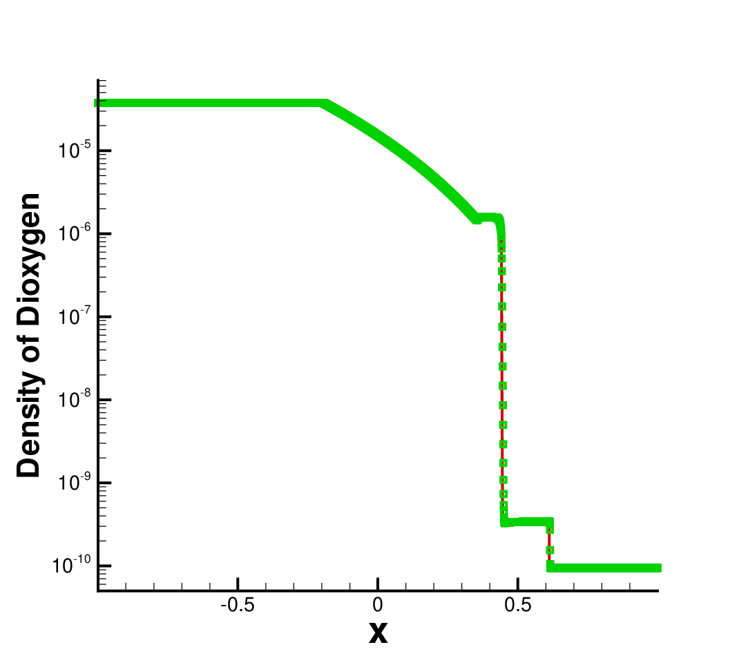
General equation of state. We consider the three species model of the one-dimensional Euler system with a more general equation of state in [19, 26]. The model involves three species, , and (, and ) with the reaction
| (4.7) |
The governing equations are
| (4.8) |
and
| (4.9) |
where the enthalpy is a constant, is the universal gas constant, is the molar mass of species , and the internal energy and for monoatomic and diatomic species respectively. The rate of the chemical reaction is given by
| (4.10) | |||
| (4.11) |
The parameters and constants are , , , , and , , , , .
The eigenvalues of the Jacobian are where with . Similar to Example 4.7, the time step is chosen to be
| (4.12) |
here on all grids and is
| (4.13) |
A shock tube problem is considered for the reactive flows with high pressure on the left and low pressure on the right initially in the chemical equilibrium (). The initial conditions are:
| (4.14) |
with zero velocity everywhere and the densities satisfying
| (4.15) |
where , and . The initial densities of , and are , and on the left respectively, and , and on the right respectively.
The numerical solution with the PP flux limiter is computed on a mesh size of up to . is taken as in [26]. In Fig. 4.6, the positivity of , , and is preserved and converged solutions are observed.

,
 ,
,


5 Conclusion
We addressed the potential negative density and pressure problem that emerges when the high order WENO schemes are applied to solve compressible Euler equations in some extreme situations. The approach that we propose is in the conservative high order finite difference WENO approximation framework. We generalized the MPP flux limiting technique for the high order finite difference WENO methods solving scalar conservation law to a class of PP flux limiters for compressible Euler equations. We also developed the parametrized flux limiters for equations with source terms. Extensive numerical tests show the capability of the proposed approach: without sacrificing accuracy and much of the efficiency, the new schemes produce solutions satisfying the PP property for scalar problems with a source term, and solutions with positive density and pressure for compressible Euler equations with or without source terms.
Acknowledgement. We would like to thank Xiangxiong Zhang from MIT for helpful discussions.
References
- [1] J. P. Boris and D. L. Book, Flux-corrected transport. I. SHASTA, A fluid transport algorithm that works, Journal of computational physics, 11 (1973), pp. 38–69.
- [2] S. R. Chakravarthy and S. Osher, High resolution applications of the Osher upwind scheme for the Euler equations, AIAA, (1983).
- [3] B. Einfeldt, C.-D. Munz, P. L. Roe, and B. Sjögreen, On Godunov-type methods near low densities, Journal of computational physics, 92 (1991), pp. 273–295.
- [4] B. Engquist and S. Osher, Stable and entropy satisfying approximations for transonic flow calculations, Mathematics of Computation, 34 (1980), pp. 45–75.
- [5] Y. Ha and C. L. Gardner, Positive scheme numerical simulation of high mach number astrophysical jets, Journal of Scientific Computing, 34 (2008), pp. 247–259.
- [6] A. Harten, B. Engquist, S. Osher, and S. R. Chakravarthy, Uniformly high order accurate essentially non-oscillatory schemes, III, Journal of Computational Physics, 71 (1987), pp. 231–303.
- [7] C. Hu and C.-W. Shu, Weighted essentially non-oscillatory schemes on triangular meshes, Journal of Computational Physics, 150 (1999), pp. 97–127.
- [8] X. Y. Hu, N. A. Adams, and C.-W. Shu, Positivity-preserving method for high-order conservative schemes solving compressible Euler equations, Journal of Computational Physics, 242 (2013), pp. 169–180.
- [9] G.-S. Jiang and C.-W. Shu, Efficient implementation of weighted ENO schemes, Journal of Computational Physics, 126 (1996), pp. 202–228.
- [10] C. Liang and Z. Xu, Parametrized maximum principle preserving flux limiters for high order schemes solving multi-dimensional scalar hyperbolic conservation laws, Journal of Scientific Computing, (2013).
- [11] T. Linde and P. L. Roe, Robust Euler codes, in Thirteenth Computational Fluid Dynamics Conference, AIAA Paper-97-2098, 1997.
- [12] X.-D. Liu and S. Osher, Nonoscillatory high order accurate self-similar maximum principle satisfying shock capturing schemes I, SIAM Journal on Numerical Analysis, 33 (1996), pp. 760–779.
- [13] B. Perthame and C.-W. Shu, On positivity preserving finite volume schemes for Euler equations, Numerische Mathematik, 73 (1996), pp. 119–130.
- [14] C.-W. Shu, Essentially non-oscillatory and weighted essentially non-oscillatory schemes for hyperbolic conservation laws, Advanced numerical approximation of nonlinear hyperbolic equations, (1998), pp. 325–432.
- [15] C.-W. Shu and S. Osher, Efficient implementation of essentially non-oscillatory shock-capturing schemes, Journal of Computational Physics, 77 (1988), pp. 439–471.
- [16] P. K. Sweby, High resolution schemes using flux limiters for hyperbolic conservation laws, SIAM journal on numerical analysis, 21 (1984), pp. 995–1011.
- [17] B. Van Leer, Towards the ultimate conservative difference scheme. II. monotonicity and conservation combined in a second-order scheme, Journal of computational physics, 14 (1974), pp. 361–370.
- [18] C. Wang, X. Zhang, C.-W. Shu, and J. Ning, Robust high order discontinuous Galerkin schemes for two-dimensional gaseous detonations, Journal of Computational Physics, 231 (2012), pp. 653–665.
- [19] W. Wang, C.-W. Shu, H. Yee, and B. Sjögreen, High-order well-balanced schemes and applications to non-equilibrium flow, Journal of Computational Physics, 228 (2009), pp. 6682–6702.
- [20] T. Xiong, J.-M. Qiu, and Z. Xu, A parametrized maximum principle preserving flux limiter for finite difference RK-WENO schemes with applications in incompressible flows , Journal of Computational Physics, 252 (2013), pp. 310–331.
- [21] T. Xiong, J.-M. Qiu, Z. Xu, and A. Christlieb, High order maximum principle preserving Semi-Lagrangian finite difference WENO schemes for the Vlasov equation, arXiv:1401.0076, (submitted, 2013).
- [22] Z. Xu, Parametrized maximum principle preserving flux limiters for high order scheme solving hyperbolic conservation laws: one-dimensional scalar problem, Mathematics of Computation, (in press.).
- [23] X. Zhang and C.-W. Shu, On positivity-preserving high order discontinuous Galerkin schemes for compressible Euler equations on rectangular meshes, Journal of Computational Physics, 229 (2010), pp. 8918–8934.
- [24] , Maximum-principle-satisfying and positivity-preserving high-order schemes for conservation laws: survey and new developments, Proceedings of the Royal Society A: Mathematical, Physical and Engineering Science, 467 (2011), pp. 2752–2776.
- [25] X. Zhang and C.-W. Shu, Positivity-preserving high order discontinuous Galerkin schemes for compressible Euler equations with source terms, Journal of Computational Physics, 230 (2011), pp. 1238–1248.
- [26] X. Zhang and C.-W. Shu, Positivity-preserving high order finite difference WENO schemes for compressible Euler equations, Journal of Computational Physics, 231 (2012), pp. 2245–2258.