Self-forced evolutions of an implicit rotating source: A natural framework to model comparable and intermediate mass–ratio systems from inspiral through ringdown

We model the inspiral phase evolution in the context of the Effective One Body (EOB) formalism [64], i.e., we consider the scenario in which the dynamics of a binary system is mapped onto the motion of a test particle in a time-independent and spherically symmetric Schwarzschild space-time with total mass $M$:

$$\mathrm{d}s^{2}_{\rm{EOB}}=-A(r)\mathrm{d}t^{2}+B(r)\mathrm{d}t^{2}+r^{2}\mathrm{d}\Omega^{2}\,,$$

(2)

where the potentials $A,\,B$ are known to 3PN order [65, 66]. In the test-mass particle limit $\eta\rightarrow 0$, these potentials recover the Schwarzschild results, namely:

$$A(u,\eta\rightarrow 0)=B^{-1}(u,\eta\rightarrow 0)=1-2\,u,\quad{\rm{with}}\quad u=\frac{M}{r}.$$

(3)

In the EOB formalism, the orbital frequency evolution can be derived from a Hamiltonian, $H_{\rm{EOB}}$ [64], given by:

$$H_{\rm{EOB}}=M\sqrt{1+2\,\eta\left(H_{\rm{eff}}-1\right)},$$

(4)

using the general Hamiltonian equation:

$$\frac{d\phi}{d\mathrm{t}}=M\Omega=\frac{\partial H_{\rm{EOB}}}{\partial L}=\frac{u^{2}\,L(x)\,A(u)}{H(u)\,H_{\rm{eff}}(u)},$$

(5)

where

	$\displaystyle H_{\rm{eff}}(u)$	$\displaystyle=$	$\displaystyle\frac{A(u)}{\sqrt{\tilde{A}(u)}}\,,\qquad\tilde{A}(u)=A(u)+\frac{1}{2}\,u\,A^{\prime}(u),$		(6)
			$\displaystyle{\rm{and}}\,\,\quad H(u)=\sqrt{1+2\,\eta\left(H_{\rm{eff}}-1\right)}.$

Recent work in the self-force formalism has enabled the derivation of gravitational self-force corrections to the EOB potential $A(u)\rightarrow 1-2u+\eta\,a(u)+{\cal{O}}(\eta^{2})$ [67]. Deriving this gravitational self-force contribution, $a(u)$, is equivalent to including all PN corrections to the EOB potential $A(u)$ at linear order in $\eta$. We shall now briefly describe the construction of the gravitational self-force contribution $a(u)$, emphasizing the fact that this contribution encodes information about the strong-field regime of the gravitational field.

As shown by Detweiler and Whiting [68], the gravitational self-force corrected worldline can be interpreted as a geodesic in a smooth perturbed spacetime with metric

$$g_{\alpha\beta}=g^{0}_{\alpha\beta}(m_{2})+h^{R}_{\alpha\beta},$$

(7)

where the regularized $R$ field is a smooth perturbation associated with $m_{1}$. Detweiler proposed a gauge invariant relation to handle the conservative effect of the gravitational self-force in circular motion [69, 70]:

$$z_{1}(\Omega)=\sqrt{1-3x}\left(1-\frac{1}{2}h^{R,\,F}_{uu}+q\frac{x}{1-3x}\right),$$

(8)

where $x$ is the gauge-invariant dimensionless frequency parameter given by $x=\left(M\Omega\right)^{2/3}$, $h^{R,\,G}_{uu}$ is a double contraction of the regularised metric perturbation with the four-velocity, $u^{\mu}$, $h^{R,\,G}_{uu}=h^{R,\,G}_{\mu\nu}u^{\mu}u^{\nu}$, the label $G$ indicates the gauge used to evaluate the metric perturbation and the label $F$ indicates that this expression is valid within the class of asymptotically flat gauges. In [1], $z_{1}(\Omega)$ was calculated in Lorenz gauge and the following gauge transformation can be used to link the asymptotically flat $h^{R,\,F}_{uu}$ metric perturbation to its Lorenz-gauge counterpart $h^{R,\,L}_{uu}$:

$$h^{R,\,F}_{uu}=h^{R,\,L}_{uu}+2q\frac{x(1-2x)}{\left(1-3x)\right)^{3/2}}.$$

(9)

Hence, inserting Eq. (9) into Eq. (8) leads to

$$z_{1}(\Omega)=\sqrt{1-3x}\left(1-\frac{1}{2}h^{R,\,L}_{uu}-2q\frac{x(1-2x)}{\left(1-3x)\right)^{3/2}}+q\frac{x}{1-3x}\right).$$

(10)

The numerical data obtained in [1] for $h^{R,\,L}_{uu}$ from $x>1/5$ was new and the numerical accuracy for $x<1/5$ was also much improved compared to previous results [69, 71]. The EoB potential $a(x)$ can be constructed from $h_{uu}^{R,L}$ via

$$a(x)=-\frac{1}{2}\left(1-3x\right)\tilde{h}^{R,\,L}_{uu}-2x\sqrt{1-3x},$$

(11)

with $\tilde{h}^{R,\,L}_{uu}=q^{-1}h^{R,\,L}_{uu}$. In [1], a global fit formula for $a(x)$ was given a dense sample of numerical values over the entire range $0<x<\frac{1}{3}$. The numerical fit for $a(x)$ that we use in this study is taken from Eq.(54) of [1]. This global analytic fit for $a(x)$ can be recast using the relation

$$a(x)=2x^{3}\,\frac{(1-2x)}{\sqrt{1-3x}}\,a_{E}(x).$$

(12)

Using the above dictionary, the model for $a(x)$ in this paper reproduces the numerical data points for the function $a_{E}(x)$ to within a maximal absolute difference of $1.2\times 10^{-5}$ over the domain $0<x<\frac{1}{3}$. The corresponding self-force corrected energy and angular momentum are given by [1, 67]

	$\displaystyle E(u(x))$	$\displaystyle=$	$\displaystyle E_{0}(x)+\eta\left(-\frac{1}{3}\frac{x}{\sqrt{1-3x}}a^{\prime}(x)+\frac{1}{2}\frac{1-4x}{\left(1-3x\right)^{3/2}}a(x)-E_{0}(x)\left(\frac{1}{2}E_{0}(x)+\frac{x}{3}\frac{1-6x}{\left(1-3x\right)^{3/2}}\right)\right),$		(13)
	$\displaystyle L_{z}(u(x))$	$\displaystyle=$	$\displaystyle L_{0}(x)+\eta\left(-\frac{1}{3}\frac{x}{\sqrt{x(1-3x)}}a^{\prime}(x)-\frac{1}{2}\frac{1}{\sqrt{x}\left(1-3x\right)^{3/2}}a(x)-\frac{1}{3}\frac{1-6x}{\sqrt{x}\left(1-3x\right)^{3/2}}\left(E_{0}(x)-1\right)\right)\,,$		(14)
			$\displaystyle{\rm{with}}\qquad\qquad u(x)=x\left(1+\eta\Bigg[\frac{1}{6}a^{\prime}(x)+\frac{2}{3}\left(\frac{1-2x}{\sqrt{1-3x}}-1\right)\Bigg]\right)\,,$		(15)

where $E_{0}(x)$ and $L_{0}(x)$ are given by

	$\displaystyle E_{0}(x)$	$\displaystyle=$	$\displaystyle\frac{1-2x}{\sqrt{1-3x}}-1,$		(16)
	$\displaystyle L_{0}(x)$	$\displaystyle=$	$\displaystyle\frac{1}{\sqrt{x(1-3x)}}.$		(17)

In Figure 3, we show the effect of these conservative corrections on the orbital parameters.

As discussed in [67], if one makes use of the self-force expression for the energy given by Eq. (13), and minimize it with respect to the orbital frequency, then one finds that binary systems with mass-ratios $q\in[1,\,1/2,\,1/3]$ do not have an ISCO in this model. It was argued in [67] that deriving self-force results in the strong field regime may alleviate this problem. We have explored this issue, and have found that using linear self-force corrections that are valid all the way to the light ring (last unstable circular orbit for massless particles) does not fix this problem for comparable mass-ratio systems. In Figure 4, we show that the existence of an ISCO is guaranteed for BH binaries with symmetric mass-ratio $\eta\mathrel{\hbox{\hbox to0.0pt{\hbox{\lower 4.0pt\hbox{$\sim$}}\hss}\hbox{$<$}}}6/49\,({\rm{or}}\,q\mathrel{\hbox{\hbox to0.0pt{\hbox{\lower 4.0pt\hbox{$\sim$}}\hss}\hbox{$<$}}}1/6)$, and its location may be approximated by

$$x_{\mathrm{ISCO}}=\frac{1}{6}\left(1+0.83401\eta+4.59483\eta^{2}\right).$$

(18)

It remains to be seen whether the inclusion of second-order conservative corrections gives an ISCO for binaries with mass-ratios $q\mathrel{\hbox{\hbox to0.0pt{\hbox{\lower 4.0pt\hbox{$\sim$}}\hss}\hbox{$>$}}}1/6$.

We include higher-order in mass-ratio terms using the exponential resummation approach described in [72]. In this approach, the energy flux is

$\displaystyle\left(\frac{{\mathrm{d}}E}{{\mathrm{d}}t}\right)_{\rm hybrid}$

$\displaystyle=$

$\displaystyle{\cal{L}}_{\rm 0}\exp\left({\cal{L}}_{\eta}\right)\,,$

(20)

where ${\cal{L}}_{\rm 0}$ denotes the leading-order in mass-ratio PN energy flux given in Eq. (19), and ${\cal{L}}_{\eta}$ incorporates mass-ratio corrections to the highest PN order available [75, 76, 72], and additional corrections characterised by a set of unknown coefficients, $b_{i}$

	$\displaystyle{\cal{L}}_{\eta}$	$\displaystyle=$	$\displaystyle\Bigg[x\bigg[-\frac{35}{12}\eta+b_{1}\,\eta^{2}\bigg]+4\pi x^{3/2}\bigg[b_{2}\,\eta+b_{3}\eta^{2}\bigg]+x^{2}\bigg[\frac{9271}{504}\eta+\frac{65}{18}\eta^{2}\bigg]+\pi x^{5/2}\bigg[-\frac{583}{24}\eta+b_{4}\,\eta^{2}\bigg]$		(21)
		$\displaystyle+$	$\displaystyle x^{3}\bigg[\eta\left(-\frac{134\,543}{7\,776}+\frac{41}{48}\pi^{2}\right)-\frac{94403}{3024}\eta^{2}-\frac{775}{324}\eta^{3}\bigg]+\pi x^{7/2}\bigg[\frac{214745}{1728}\eta+\frac{193385}{3024}\eta^{2}\bigg]\Bigg].$

The coefficients $b_{i}$ were taken to be constant in [72], but we found that a better match to the EOB phase evolution could be obtained by allowing an additional dependence on mass-ratio in these terms (see Eqs. (23)-(25) below). We constrain the $b_{i}$ coefficients by ensuring that the phase evolution of this model reproduces the phase evolution predicted by the EOB model introduced in [2, 3], which was calibrated to the phase evolution of compact binaries observed in numerical relativity simulations. To do so, we implemented the EOB model [2] and performed a Monte Carlo simulation to optimize the values of the $b_{i}$ coefficients (see Figure 5). The optimization was done in two stages. We started by considering the three coefficients $b_{1},\,b_{2}$ and $b_{4}$, sampling a wide range of parameter space, namely $b_{i}\in[-200,200]$. We constrained the duration of the waveform from early inspiral to the light-ring to be similar to its EOB counterpart. Waveforms that differed from their EOB counterparts by more than $10^{-4}$ seconds were discarded. Once the region under consideration had been sparsely sampled, we focused on regions of parameter space where the orbital phase evolution was closest to the EOB evolution, and finely sampled these to obtain the optimal values for the coefficients. We found that this approach enabled us to reproduce the EOB phase evolution with a phase discrepancy of the order $\sim 1$ rad. After constraining $b_{1},\,b_{2}$ and $b_{4}$, we explored whether including additional corrections could further improve the phase evolution, by adding $\eta$ corrections beyond 3PN order. Such corrections were found to have a negligible impact on the actual phase evolution. This is not difficult to understand, since such corrections are of order $({\cal{O}}(\eta^{4}),\,{\cal{O}}(\eta^{3}))$, at (3PN, 3.5PN) respectively. We found a similar behavior when we added leading order mass-ratios corrections beyond 4PN order. Thus, we took a different approach: having derived the optimal value for $b_{1},\,b_{2}$ and $b_{4}$, we took these results as initial seeds for an additional MC simulation in which $b_{3}$ was also included in Eq. (21), and repeated the optimization procedure. The results of these simulations are shown in Figure 5.

	$\displaystyle{\cal{L}}_{\eta}$	$\displaystyle=$	$\displaystyle\Bigg[x\bigg[-\frac{35}{12}\eta+B_{1}\bigg]+4\pi x^{3/2}B_{2}+x^{2}\bigg[\frac{9271}{504}\eta+\frac{65}{18}\eta^{2}\bigg]+\pi x^{5/2}\bigg[-\frac{583}{24}\eta+B_{3}\bigg]$		(22)
		$\displaystyle+$	$\displaystyle x^{3}\bigg[\eta\left(-\frac{134\,543}{7\,776}+\frac{41}{48}\pi^{2}\right)-\frac{94403}{3024}\eta^{2}-\frac{775}{324}\eta^{3}\bigg]+\pi x^{7/2}\bigg[\frac{214745}{1728}\eta+\frac{193385}{3024}\eta^{2}\bigg]\Bigg].$

where:

where we have used the mass-ratio corrected energy —Eq. (13)— to compute ${\mathrm{d}}E/{\mathrm{d}}x$. Figure 6 shows that for binaries with mass-ratio $q=1/6$, the phase discrepancy between our self-force model and EOB is $\mathrel{\hbox{\hbox to0.0pt{\hbox{\lower 4.0pt\hbox{$\sim$}}\hss}\hbox{$<$}}}0.5$ rads at the light-ring, which is within the numerical accuracy of the simulations used to calibrate EOB. It has been shown recently that EOB remains accurate for mass-ratios up to $q=1/8$ [77]. In that regime the phase discrepancy between this model and EOB at the light-ring is less than 1 rad, as shown in Figure 6. For binaries with $q=1/10$, the phase discrepancy at the light-ring is $\mathrel{\hbox{\hbox to0.0pt{\hbox{\lower 4.0pt\hbox{$\sim$}}\hss}\hbox{$<$}}}1.2$ rads, which is still within the numerical accuracy of available simulations [78, 79].

If only the leading-order modes $(\ell,m)=(2,\pm 2)$ and included, the inspiral waveform components are given by

	$\displaystyle h_{+}(t)$	$\displaystyle=$	$\displaystyle\frac{4\,\mu\,r^{2}\,\dot{\phi}^{2}}{D}\left(\frac{1+\cos^{2}\iota}{2}\right)\cos\left[2(\phi(t)+\Phi)\right],$		(28)
	$\displaystyle h_{\times}(t)$	$\displaystyle=$	$\displaystyle\frac{4\,\mu\,r^{2}\,\dot{\phi}^{2}}{D}\cos\iota\sin\left[2(\phi(t)+\Phi)\right],$		(29)

where $D$ is the distance to the source. Since the orbital evolution will deviate from a circular trajectory during late inspiral ($\dot{r}\neq 0$), we must consider more general orbits in which both $\dot{r}$ and $\dot{r}\dot{\phi}$ are non-negligible. For such orbits, the Newtonian GW polarizations are given by [86]:

	$\displaystyle h_{+}(t)$	$\displaystyle=$	$\displaystyle\frac{2\mu}{D}\Bigg\{\left(1+\cos^{2}\iota\right)\Bigg[\cos\left[2(\phi(t)+\Phi)\right]\left(-\dot{r}^{2}+r^{2}\dot{\phi}^{2}+\frac{1}{r}\right)$		(30)
		$\displaystyle+$	$\displaystyle 2r\,\dot{r}\,\dot{\phi}\,\sin\left[2(\phi(t)+\Phi)\right]\Bigg]+\left(-\dot{r}^{2}-r^{2}\dot{\phi}^{2}+\frac{1}{r}\right)\sin^{2}\iota\Bigg\}\,,$
	$\displaystyle h_{\times}(t)$	$\displaystyle=$	$\displaystyle\frac{4\mu}{D}\cos\iota\Bigg\{\sin\left[2(\phi(t)+\Phi)\right]\left(-\dot{r}^{2}+r^{2}\dot{\phi}^{2}+\frac{1}{r}\right)$		(31)
		$\displaystyle-$	$\displaystyle 2r\,\dot{r}\,\dot{\phi}\,\cos\left[2(\phi(t)+\Phi)\right]\Bigg\},$

where $\dot{r}$ can be computed using

$$\frac{{\mathrm{d}}r}{{\mathrm{d}}t}=-\frac{1}{u^{2}}\frac{{\mathrm{d}u}}{{\mathrm{d}}x}\frac{{\mathrm{d}x}}{{\mathrm{d}}t}\,.$$

Having described the construction of the inspiral evolution, we shall now describe the approach followed to smoothly connect the late inspiral evolution onto the plunge phase. The adiabatic prescription given by Eq. (26) breaks down when $dE/dx\rightarrow 0$. Hence, we need a scheme that enables us to match the late inspiral phase onto the plunge phase. We will do this by modifying the “transition” phase developed by Ori and Thorne [4] by including finite mass–ratio corrections.

In this Section we describe an extension of the transition phase model introduced by Ori and Thorne [4]. The basic idea behind this approach can be understood by studying the motion of an inspiralling object in terms of the effective potential, $V(r,L)$, which takes the following simple form for a Schwarzschild BH [87]:

$$V(r,L)=\left(1-\frac{2}{r}\right)\left(1+\frac{L^{2}}{r^{2}}\right).$$

(32)

Throughout the inspiral, the body moves along a nearly circular orbit, and hence the radio of the energy flux to the angular momentum flux is given by:

$$\frac{{\mathrm{d}}E}{{\mathrm{d}}\tau}=\Omega\frac{{\mathrm{d}}L}{{\mathrm{d}}\tau}.$$

(33)

Hence, near the ISCO, the energy and angular momentum of the body satisfy the following relations:

	$\displaystyle E$	$\displaystyle\rightarrow$	$\displaystyle E_{\rm{ISCO}}+\Omega_{\rm{ISCO}}\,\xi,$		(34)
	$\displaystyle L$	$\displaystyle\rightarrow$	$\displaystyle L_{\rm{ISCO}}+\xi.$		(35)

Re-writing the effective potential, Eq. (32), in terms of $\xi=L-L_{\rm{ISCO}}$, one notices that during early inspiral, $\xi\gg 0$, the motion of the object is adiabatic, and the object sits at the minimum of the potential —as shown in the left panel of Figure 7. However, as the object nears the ISCO, the minimum of the potential moves inward due to radiation reaction. At some point, the body’s inertia prevents the body from staying at the minimum of the potential, and adiabatic inspiral breaks down [4] — illustrated in the right-hand panel of Figure 7.

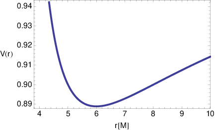
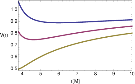
The equation that governs the radial motion during the transition regime is found by linearising the equation

$$\left(\frac{{\mathrm{d}}r}{{\mathrm{d}}\tau}\right)^{2}=E(r)^{2}-V(r,\,L),$$

(36)

using Eqs. (34), (35), and

$$\frac{{\mathrm{d}}\xi}{{\mathrm{d}}\tau}=\kappa\,\eta,\quad{\rm{with}}\quad\kappa=\bigg[\frac{32}{5}\Omega^{7/3}\frac{\dot{{\cal{E}}}}{\sqrt{1-3u}}\bigg]_{\rm{ISCO}}\,,$$

(37)

where $\dot{{\cal{E}}}$ is the general relativistic correction to the Newtonian, quadrupole-moment formula [63]. We now extend these Eqs. by including finite mass-ratio corrections. Eq. (36) can be replaced by

$$\frac{{\mathrm{d}}x}{{\mathrm{d}}t}=\frac{u^{2}(1-2u)}{E(x)}\left(\frac{{\mathrm{d}}u}{{\mathrm{d}}x}\right)^{-1}\bigg[E(x)^{2}-V\left(u(x),L(x)\right)\bigg]^{1/2},$$

(38)

where we have used

$$\frac{{\mathrm{d}}\tau}{{\mathrm{d}}t}=\frac{1-2\,u(x)}{E(x)}\,,$$

(39)

and the expressions for the energy and angular momentum are given by Eqs. (13), (14). In order to linearize Eq. (38) we replace $E(x)$ and $L(x)$ by Eqs (34) and (35) respectively.

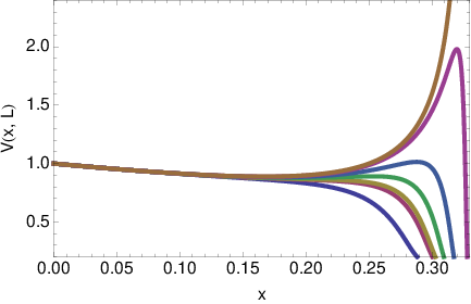
As discussed in [4], since these equations use the $\eta$-corrected values for $E(x_{\rm{ISCO}})$, $L(x_{\rm{ISCO}})$ and $\Omega_{\rm{ISCO}}$, then they remain valid even for finite mass-ratio $\eta$ [4]. In Figure 8 we show the effect that these finite mass-ratio $\eta$ corrections have on the effective potential $V(x,L(x))$. We determine the point at which the transition regime starts by carrying out a stability analysis near the ISCO using ${\mathrm{d}}E/{\mathrm{d}}x$. As shown in Figure 4, the ISCO is determined by the relation ${\mathrm{d}}E/{\mathrm{d}}x=0$. We have found that the relation

$$\left(\frac{{\mathrm{d}}E}{{\mathrm{d}}x}\right)\Bigg|_{\rm{transition}}=-0.054+\frac{1.757\times 10^{-4}}{\eta}\,,$$

(40)

provides a robust criterion to mark the start of the transition regime for binaries with mass-ratios $1/100<q<1/6$.

We model the evolution of the orbital frequency during the transition regime and thereafter in a different manner to that proposed by Ori and Thorne [4]. In order to ensure that the late-time evolution of the orbital frequency of our self-force model is as close as possible to the orbital evolution extracted from numerical relativity simulations, we incorporate the late-time frequency evolution that was derived by Baker et al [5] in their implicit rotating source (IRS) model, namely:

$$\frac{d\phi}{d\mathrm{t}}=\Omega_{\rm{i}}+\left(\Omega_{\rm{f}}\ -\Omega_{\rm{i}}\right)\left(\frac{1+\tanh(\ln\sqrt{\varkappa}+(t-t_{0})/b)}{2}\right)^{\varkappa}\,,$$

(41)

where $\Omega_{\rm{i}}$ is the value of the orbital frequency when the transition regime begins, and $\Omega_{\rm{f}}$ is the value of the frequency at the light ring, which corresponds to $\omega_{\rm{\ell mn}}/m$, where $\omega_{\rm{\ell mn}}$ is the fundamental quasi-normal ringing frequency $(n=0)$ for the fundamental mode $(\ell,m)=(2,2)$ of the post-merger black hole (see Eq. (45) below). The constant mass-dependent coefficient $t_{0}$ is computed by ensuring that $d\Omega/dt$ peaks at a time $t=t_{0}$. The parameter $\varkappa$ is computed by enforcing continuity between the first order time derivative of the orbital frequency as predicted by the self-force evolution —Eq. (5)— and that given by the first order time derivative of Eq. (41).

In Figures 9 and 10 we show the evolution obtained by combining Ori and Thorne’s [4] transition approach for the radial motion with the frequency evolution proposed by Baker et al [5]. In all the cases shown in Figures 9 and 10, the orbital frequency peaks and saturates at a value given by $\omega_{\ell mn}/m$. This can be understood if we analyze the asymptotic behavior of Eq. (41) near the light-ring, i.e.,

$$\frac{d\phi}{d\mathrm{t}}\approx\Omega_{\rm{f}}-\left(\Omega_{\rm{f}}\ -\Omega_{\rm{i}}\right)e^{-2(t-t_{0})/b}.$$

(42)

Recasting Eq. (41) in this form, enables us to identify the constant coefficient $b$ with the e-folding rate for the decay of the fundamental quasinormal mode (QNM). As discussed previously, Eq. (41) predicts the expected orbital evolution during late inspiral and onward. To provide a unified description from late inspiral through to ringdown, we have decided to adopt the IRS approach, since this framework allows us to smoothly transition from late inspiral onto the plunge phase, and finally describe the ringdown waveform as a natural consequence of the IRS strain-rate amplitude decay relation $A^{2}(t)\propto\Omega\dot{\Omega}$ [5]. In other words, since Eq. (42) has the correct behavior near the light-ring as predicted by BHPT, the IRS model provides a natural framework to attach the ringdowm waveform at the end of the plunge phase. We will discuss this feature in further detail in the following Section.

Numerical relativity simulations have shown that coalescing binary BHs in general relativity lead to the formation of a distorted rotating remnant, which radiates GWs while it settles down into a stationary Kerr BH [88, 89]. The GWs emitted during this intermediate phase resemble a ringing bell. Hence, this type of radiation is commonly known in the literature as ringdown radiation, and consists of a superposition of QNMs — first discovered in numerical studies of the scattering of GWs in the Schwarzschild spacetime by Vishveshwara [90]. QNMs are damped oscillations whose frequencies and damping times are uniquely determined by the mass and spin of the post-merger Kerr BH. The frequency $\hat{\omega}$ of each QNM has two components: the real part represents the oscillation frequency, and the imaginary part corresponds to the inverse of the damping time:

$$\hat{\omega}=\omega_{\ell mn}-i/\tau_{\ell mn}.$$

(43)

As discussed above, the observables $\omega_{\ell mn},\,\tau_{\ell mn}$ are uniquely determined by the final mass, $M_{\rm{f}}$, and final spin, $q_{\rm{f}}$, of the post-merger Kerr BH. To determine $M_{\rm{f}}$, we use the analytic phenomenological expression for the final mass of the BH remnant that results from the merger of generic binary BHs on circular quasi-orbits introduced in [91], namely,

$$\frac{M_{\rm{f}}}{M}=1-\left(1-\frac{2\sqrt{2}}{3}\right)\eta-0.543763\,\eta^{2}.$$

(44)

This expression reproduces the expected result in the test mass particle limit, and also reproduces results from currently available numerical relativity simulations [91, 92]. We determine the final spin of the BH remnant $q_{\rm{f}}$ using the fit proposed in [93]:

$$q_{\rm{f}}=\sqrt{12}\,\eta+s_{1}\,\eta^{2}+s_{2}\,\eta^{3},$$

(45)

with:

$$\displaystyle s_{1}=-3.454\pm 0.132,\qquad s_{1}=2.353\pm 0.548.$$

(46)

This prescription is consistent with the numerical relativity simulations described in [93, 92], and reproduces test mass limit predictions. This compact formula is also consistent with the prescriptions introduced in [94, 95]. The largest discrepancy between Eq. (45) and those derived in [94, 95] is $\mathrel{\hbox{\hbox to0.0pt{\hbox{\lower 4.0pt\hbox{$\sim$}}\hss}\hbox{$<$}}}2.5\%$ for binaries with $q\mathrel{\hbox{\hbox to0.0pt{\hbox{\lower 4.0pt\hbox{$\sim$}}\hss}\hbox{$<$}}}1/6$. The ringdown waveform is given by [89, 5]

$\displaystyle h(t)$

$\displaystyle=$

$\displaystyle-\left(h_{+}-ih_{\times}\right)=\frac{M_{\rm{f}}}{D}\sum_{\ell mn}{\cal{A}}_{\ell mn}\,e^{-i\left(\omega_{\ell mn}\,t+\phi_{\ell mn}\right)}\,e^{-t/\tau_{\ell mn}}\,,$

(47)

where ${\cal{A}}_{\ell mn}$ and $\phi_{\ell mn}$ are constants to be determined by smoothly matching the plunge waveform onto the subsequent ringdown. The ringdown portion of the self-force waveform model constructed in this paper includes the mode $\ell=m=2$ and the tones $n=0,\,1,\,2$. The approach we follow to attach the leading mode and overtones is the following:

Having described the ringdown waveform construction as a sum of quasinormal modes, we finish this Section by exhibiting the power of the IRS model to describe the ringdown evolution. In the IRS model, the strain-rate amplitude decay is given by [5]:

$$A^{2}(t)=16\,\pi\,\dot{E}\approx 16\,\pi\,\xi\,\Omega\,\dot{\Omega}\,.$$

(48)

Using Eq. (42), in the limit $\Omega\rightarrow\Omega_{\rm{f}}$, the amplitude decay is given by

$$A_{0}^{2}\,e^{-2t/\tau}\approx\frac{32\,\pi\,\xi\,\Omega_{\rm{f}}}{b}\left(\Omega_{\rm{f}}-\Omega_{\rm{i}}\right)e^{-2(t-t_{0})/\tau}\,.$$

(49)

Hence, the late-time amplitude in the IRS model is given by

$$A^{2}_{\ell m}\approx 16\,\pi\,\xi_{\ell m}\,\omega_{\ell m}\,\dot{\omega}_{\ell m}\,,$$

(50)

where the value of $\xi_{\ell m}$ is set by ensuring amplitude continuity at the light-ring. In Figure 12 we explicitly show the equivalence of the ringdown waveform construction both in the IRS approach and using the sum of QNMs utilized in the previous Section. This detailed analysis shows that the IRS is a powerful tool to model the late time portions of the waveforms in a unified way.

References

- [1] S. Akcay, L. Barack, T. Damour, and N. Sago, Phys. Rev. D 86, 104041 (2012), arXiv:1209.0964 [gr-qc] .
- [2] Y. Pan, A. Buonanno, M. Boyle, L. T. Buchman, L. E. Kidder, H. P. Pfeiffer, and M. A. Scheel, Phys. Rev. D 84, 124052 (2011), arXiv:1106.1021 [gr-qc] .
- [3] T. Damour, A. Nagar, and S. Bernuzzi, Phys. Rev. D 87, 084035 (2013), arXiv:1212.4357 [gr-qc] .
- [4] A. Ori and K. S. Thorne, Phys. Rev. D 62, 124022 (2000), arXiv:gr-qc/0003032 .
- [5] J. G. Baker, W. D. Boggs, J. Centrella, B. J. Kelly, S. T. McWilliams, and J. R. van Meter, Phys. Rev. D 78, 044046 (2008), arXiv:0805.1428 [gr-qc] .
- [6] J. E. McClintock and R. A. Remillard, “Black hole binaries,” in Compact stellar X-ray sources, edited by W. H. G. Lewin and M. van der Klis (2006) pp. 157–213.
- [7] M. Morscher, S. Umbreit, W. M. Farr, and F. A. Rasio, Astrophys. J. Lett 763, L15 (2013), arXiv:1211.3372 [astro-ph.GA] .
- [8] A. Merloni and S. Heinz, MNRAS 388, 1011 (2008), arXiv:0805.2499 .
- [9] M. Fukugita and P. J. E. Peebles, Astrophys. J. 616, 643 (2004), arXiv:astro-ph/0406095 .
- [10] J. M. Miller, A. Zezas, G. Fabbiano, and F. Schweizer, Astrophys. J. 609, 728 (2004a), astro-ph/0302535 .
- [11] J. M. Miller, A. C. Fabian, and M. C. Miller, Astrophys. J. 607, 931 (2004b), astro-ph/0310617 .
- [12] J. M. Miller, “Present evidence for intermediate mass black holes in ULXs and future prospects,” in From X-ray Binaries to Quasars: Black Holes on All Mass Scales, edited by T. J. Maccarone, R. P. Fender, and L. C. Ho (2005) pp. 227–238.
- [13] D. A. Swartz, R. Soria, A. F. Tennant, and M. Yukita, Astrophys. J. 741, 49 (2011), arXiv:1108.1372 [astro-ph.HE] .
- [14] L. Zampieri and T. P. Roberts, MNRAS 400, 677 (2009), arXiv:0909.1017 [astro-ph.HE] .
- [15] K. Belczynski, T. Bulik, C. L. Fryer, A. Ruiter, F. Valsecchi, J. S. Vink, and J. R. Hurley, Astrophys. J. 714, 1217 (2010), arXiv:0904.2784 [astro-ph.SR] .
- [16] K. Ohsuga and S. Mineshige, Astrophys. J. 736, 2 (2011), arXiv:1105.5474 [astro-ph.HE] .
- [17] H. Matsumoto, T. G. Tsuru, K. Koyama, H. Awaki, C. R. Canizares, N. Kawai, S. Matsushita, and R. Kawabe, Astrophys. J. Lett 547, L25 (2001), arXiv:astro-ph/0009250 .
- [18] S. A. Farrell, N. A. Webb, D. Barret, O. Godet, and J. M. Rodrigues, Nature (London) 460, 73 (2009), arXiv:1001.0567 [astro-ph.HE] .
- [19] F. P. A. Wolter Ginevra Trinchieri, ArXiv e-prints (2010), arXiv:1003.4671 [astro-ph.HE] .
- [20] P. G. Jonker, M. A. P. Torres, A. C. Fabian, M. Heida, G. Miniutti, and D. Pooley, MNRAS 407, 645 (2010), arXiv:1004.5379 [astro-ph.HE] .
- [21] S. F. Portegies Zwart, H. Baumgardt, P. Hut, J. Makino, and S. L. W. McMillan, Nature (London) 428, 724 (2004), arXiv:astro-ph/0402622 .
- [22] T. E. Strohmayer and R. F. Mushotzky, Astrophys. J. Lett 586, L61 (2003), arXiv:astro-ph/0303665 .
- [23] P. Kaaret and H. Feng, Astrophys. J. 669, 106 (2007), arXiv:0707.2055 .
- [24] H. Feng and P. Kaaret, Astrophys. J. Lett 712, L169 (2010), arXiv:1003.0283 [astro-ph.HE] .
- [25] A. D. Sutton, T. P. Roberts, D. J. Walton, J. C. Gladstone, and A. E. Scott, MNRAS 423, 1154 (2012), arXiv:1203.4100 [astro-ph.HE] .
- [26] M. Trenti, ArXiv Astrophysics e-prints (2006), arXiv:astro-ph/0612040 .
- [27] M. Coleman Miller and E. J. M. Colbert, International Journal of Modern Physics D 13, 1 (2004), arXiv:astro-ph/0308402 .
- [28] M. Volonteri, A&ARv 18, 279 (2010), arXiv:1003.4404 [astro-ph.CO] .
- [29] R. Schneider, A. Ferrara, P. Natarajan, and K. Omukai, Astrophys. J. 571, 30 (2002), arXiv:astro-ph/0111341 .
- [30] Q. Yu and S. Tremaine, MNRAS 335, 965 (2002), arXiv:astro-ph/0203082 .
- [31] I. Mandel, ArXiv e-prints (2007), arXiv:0707.0711 .
- [32] G. M. Harry and LIGO Scientific Collaboration, Class. Quantum Grav. 27, 084006 (2010).
- [33] F. Acernese et al., Class. Quantum Grav. 25, 184001 (2008).
- [34] K. Somiya and the KAGRA Collaboration, Class. Quantum Grav. 29, 124007 (2012).
- [35] D. Shoemaker, “Advanced LIGO anticipated sensitivity curves,” (2010), https://dcc.ligo.org/cgi-bin/DocDB/ShowDocument?docid=2974.
- [36] A. Freise, S. Chelkowski, S. Hild, W. Del Pozzo, A. Perreca, and A. Vecchio, Class. Quantum Grav. 26, 085012 (2009), arXiv:0804.1036 .
- [37] J. R. Gair, I. Mandel, M. C. Miller, and M. Volonteri, General Relativity and Gravitation 43, 485 (2011), arXiv:0907.5450 [astro-ph.CO] .
- [38] E. A. Huerta and J. R. Gair, Phys. Rev. D 83, 044020 (2011a), arXiv:1009.1985 [gr-qc] .
- [39] E. A. Huerta and J. R. Gair, Phys. Rev. D 83, 044021 (2011b), arXiv:1011.0421 [gr-qc] .
- [40] Y. Taniguchi, Y. Shioya, T. G. Tsuru, and S. Ikeuchi, PASJ 52, 533 (2000), arXiv:astro-ph/0002389 .
- [41] M. C. Miller and D. P. Hamilton, Astrophys. J. 576, 894 (2002), arXiv:astro-ph/0202298 .
- [42] H. Mouri and Y. Taniguchi, Astrophys. J. Lett 566, L17 (2002a), arXiv:astro-ph/0201102 .
- [43] H. Mouri and Y. Taniguchi, Astrophys. J. 580, 844 (2002b), arXiv:astro-ph/0208053 .
- [44] K. Gültekin, M. C. Miller, and D. P. Hamilton, Astrophys. J. 616, 221 (2004), arXiv:astro-ph/0402532 .
- [45] K. Gültekin, M. C. Miller, and D. P. Hamilton, Astrophys. J. 640, 156 (2006), arXiv:astro-ph/0509885 .
- [46] R. M. O’Leary, F. A. Rasio, J. M. Fregeau, N. Ivanova, and R. O’Shaughnessy, Astrophys. J. 637, 937 (2006), arXiv:astro-ph/0508224 .
- [47] R. M. O’Leary, R. O’Shaughnessy, and F. A. Rasio, Phys. Rev. D 76, 061504 (2007), arXiv:astro-ph/0701887 .
- [48] I. Mandel, D. A. Brown, J. R. Gair, and M. C. Miller, Astrophys. J. 681, 1431 (2008), arXiv:0705.0285 .
- [49] J. Abadie, B. P. Abbott, R. Abbott, M. Abernathy, T. Accadia, F. Acernese, C. Adams, R. Adhikari, P. Ajith, B. Allen, et al., Class. Quantum Grav. 27, 173001 (2010), arXiv:1003.2480 [astro-ph.HE] .
- [50] R. J. E. Smith, I. Mandel, and A. Vecchio, Phys. Rev. D 88, 044010 (2013), arXiv:1302.6049 [astro-ph.HE] .
- [51] E. A. Huerta, P. Kumar, and D. A. Brown, Phys. Rev. D 86, 024024 (2012a), arXiv:1205.5562 [gr-qc] .
- [52] L. Barack, Class. Quantum Grav. 26, 213001 (2009), arXiv:0908.1664 [gr-qc] .
- [53] E. Poisson, A. Pound, and I. Vega, Living Reviews in Relativity 14, 7 (2011), arXiv:1102.0529 [gr-qc] .
- [54] E. A. Huerta and J. R. Gair, Phys. Rev. D 79, 084021 (2009), arXiv:0812.4208 .
- [55] E. A. Huerta and J. R. Gair, ArXiv e-prints (2010), arXiv:1009.5882 [gr-qc] .
- [56] E. A. Huerta and J. R. Gair, Phys. Rev. D 84, 049903 (2011c).
- [57] A. H. Mroue, M. A. Scheel, B. Szilagyi, H. P. Pfeiffer, M. Boyle, D. A. Hemberger, L. E. Kidder, G. Lovelace, S. Ossokine, N. W. Taylor, A. Zenginoglu, L. T. Buchman, T. Chu, E. Foley, M. Giesler, R. Owen, and S. A. Teukolsky, ArXiv e-prints (2013), arXiv:1304.6077 [gr-qc] .
- [58] A. Le Tiec, E. Barausse, and A. Buonanno, Phys.Rev. Lett 108, 131103 (2012), arXiv:1111.5609 [gr-qc] .
- [59] LIGO Scientific Collaboration, Virgo Collaboration, J. Aasi, J. Abadie, B. P. Abbott, R. Abbott, T. D. Abbott, M. Abernathy, T. Accadia, F. Acernese, et al., ArXiv e-prints (2013), arXiv:1304.0670 [gr-qc] .
- [60] A. Buonanno, B. R. Iyer, E. Ochsner, Y. Pan, and B. S. Sathyaprakash, Phys. Rev. D 80, 084043 (2009).
- [61] A. H. Nitz, A. Lundgren, D. A. Brown, E. Ochsner, et al., ArXiv e-prints (2013), arXiv:1307.1757 [gr-qc] .
- [62] A. Buonanno, Y. Chen, Y. Pan, H. Tagoshi, and M. Vallisneri, Phys. Rev. D 72, 084027 (2005), gr-qc/0508064 .
- [63] D. Kennefick and A. Ori, Phys. Rev. D 53, 4319 (1996), arXiv:gr-qc/9512018 .
- [64] T. Damour, Phys. Rev. D 64, 124013 (2001).
- [65] A. Buonanno and T. Damour, Phys. Rev. D 59, 084006 (1999), gr-qc/9811091 .
- [66] T. Damour, P. Jaranowski, and G. Schäfer, Phys. Rev. D 62, 084011 (2000), gr-qc/0005034 .
- [67] E. Barausse, A. Buonanno, and A. Le Tiec, Phys. Rev. D 85, 064010 (2012a), arXiv:1111.5610 [gr-qc] .
- [68] S. Detweiler and B. F. Whiting, Phys. Rev. D 67, 024025 (2003), gr-qc/0202086 .
- [69] S. Detweiler, Phys. Rev. D 77, 124026 (2008), arXiv:0804.3529 [gr-qc] .
- [70] S. Detweiler, ArXiv e-prints (2009), arXiv:0908.4363 [gr-qc] .
- [71] N. Sago, L. Barack, and S. Detweiler, Phys. Rev. D 78, 124024 (2008), arXiv:0810.2530 [gr-qc] .
- [72] S. Isoyama, R. Fujita, N. Sago, H. Tagoshi, and T. Tanaka, Phys. Rev. D 87, 024010 (2013), arXiv:1210.2569 [gr-qc] .
- [73] L. M. Burko and G. Khanna, Phys. Rev. D 88, 024002 (2013), arXiv:1304.5296 [gr-qc] .
- [74] R. Fujita, Progress of Theoretical Physics 128, 971 (2012), arXiv:1211.5535 [gr-qc] .
- [75] L. Blanchet, G. Faye, B. R. Iyer, and B. Joguet, Phys. Rev. D 65, 061501 (2002), arXiv:gr-qc/0105099 .
- [76] L. Blanchet, A. Buonanno, and G. Faye, Phys. Rev. D 84, 064041 (2011), arXiv:1104.5659 [gr-qc] .
- [77] Y. Pan, A. Buonanno, A. Taracchini, M. Boyle, L. E. Kidder, A. H. Mroue, H. P. Pfeiffer, M. A. Scheel, B. Szilagyi, and A. Zenginoglu, ArXiv e-prints (2013), arXiv:1311.2565 [gr-qc] .
- [78] C. O. Lousto, H. Nakano, Y. Zlochower, and M. Campanelli, Phys. Rev. D 82, 104057 (2010), arXiv:1008.4360 [gr-qc] .
- [79] H. Nakano, Y. Zlochower, C. O. Lousto, and M. Campanelli, Phys. Rev. D 84, 124006 (2011), arXiv:1108.4421 [gr-qc] .
- [80] N. Warburton, S. Akcay, L. Barack, J. R. Gair, and N. Sago, Phys. Rev. D 85, 061501 (2012), arXiv:1111.6908 [gr-qc] .
- [81] L. Barack and C. Cutler, Phys. Rev. D 69, 082005 (2004), arXiv:gr-qc/0310125 .
- [82] J. R. Gair, L. Barack, T. Creighton, C. Cutler, S. L. Larson, E. S. Phinney, and M. Vallisneri, Class. Quantum Grav. 21, 1595 (2004).
- [83] J. R. Gair, M. Vallisneri, S. L. Larson, and J. G. Baker, Living Reviews in Relativity 16, 7 (2013), arXiv:1212.5575 [gr-qc] .
- [84] E. A. Huerta, J. R. Gair, and D. A. Brown, Phys. Rev. D 85, 064023 (2012b), arXiv:1111.3243 [gr-qc] .
- [85] E. A. Huerta and J. R. Gair, Phys. Rev. D 84, 064023 (2011d), arXiv:1105.3567 [gr-qc] .
- [86] A. Gopakumar and B. R. Iyer, Phys. Rev. D 65, 084011 (2002), gr-qc/0110100 .
- [87] C. W. Misner, K. S. Thorne, and J. A. Wheeler, Gravitation (San Francisco: W.H. Freeman and Co., 1973, 1973).
- [88] E. Berti, V. Cardoso, and M. Casals, Phys. Rev. D 73, 024013 (2006a), arXiv:gr-qc/0511111 .
- [89] E. Berti, V. Cardoso, and C. M. Will, Phys. Rev. D 73, 064030 (2006b), arXiv:gr-qc/0512160 .
- [90] C. V. Vishveshwara, Nature (London) 227, 936 (1970).
- [91] E. Barausse, V. Morozova, and L. Rezzolla, Astrophys. J. 758, 63 (2012b), arXiv:1206.3803 [gr-qc] .
- [92] L. Rezzolla, P. Diener, E. N. Dorband, D. Pollney, C. Reisswig, E. Schnetter, and J. Seiler, Astrophys. J. Lett 674, L29 (2008a), arXiv:0710.3345 .
- [93] A. Buonanno, Y. Pan, J. G. Baker, J. Centrella, B. J. Kelly, S. T. McWilliams, and J. R. van Meter, Phys. Rev. D 76, 104049 (2007), arXiv:0706.3732 [gr-qc] .
- [94] E. Barausse and L. Rezzolla, Astrophys. J. Lett 704, L40 (2009), arXiv:0904.2577 [gr-qc] .
- [95] L. Rezzolla, E. Barausse, E. N. Dorband, D. Pollney, C. Reisswig, J. Seiler, and S. Husa, Phys. Rev. D 78, 044002 (2008b), arXiv:0712.3541 [gr-qc] .
- [96] D. A. Brown, P. Kumar, and A. H. Nitz, Phys. Rev. D 87, 082004 (2013), arXiv:1211.6184 [gr-qc] .
- [97] F. Foucart, M. B. Deaton, M. D. Duez, L. E. Kidder, I. MacDonald, C. D. Ott, H. P. Pfeiffer, M. A. Scheel, B. Szilagyi, and S. A. Teukolsky, Phys. Rev. D 87, 084006 (2013), arXiv:1212.4810 [gr-qc] .
- [98] M. Saijo, K. Maeda, M. Shibata, and Y. Mino, Phys. Rev. D 58, 064005 (1998).
- [99] L. M. Burko, Phys. Rev. D 69, 044011 (2004), arXiv:gr-qc/0308003 .
- [100] L. Blanchet, A. Buonanno, and G. Faye, Phys. Rev. D 75, 049903 (2007).
- [101] L. Blanchet, A. Buonanno, and G. Faye, Phys. Rev. D 74, 104034 (2006), arXiv:gr-qc/0605140 .
- [102] R. M. O’Leary, B. Kocsis, and A. Loeb, MNRAS 395, 2127 (2009).
- [103] E. A. Huerta and D. A. Brown, Phys. Rev. D 87, 127501 (2013), arXiv:1301.1895 [gr-qc] .
- [104] H. Yang, F. Zhang, A. Zimmerman, and Y. Chen, ArXiv e-prints (2013), arXiv:1311.3380 [gr-qc] .
- [105] S. R. Dolan, L. Barack, and B. Wardell, Phys. Rev. D 84, 084001 (2011), arXiv:1107.0012 [gr-qc] .
- [106] A. Pound, C. Merlin, and L. Barack, ArXiv e-prints (2013), arXiv:1310.1513 [gr-qc] .
- [107] F. Zhang and B. Szilágyi, Phys. Rev. D 88, 084033 (2013), arXiv:1309.1141 [gr-qc] .