A Family of Quasisymmetry Models
Abstract
We present a one-parameter family of models for square contingency tables that interpolates between the classical quasisymmetry model and its Pearsonian analogue. Algebraically, this corresponds to deformations of toric ideals associated with graphs. Our discussion of the statistical issues centers around maximum likelihood estimation.
Keywords: square contingency tables; algebraic statistics; toric models; linear models;
maximum likelihood estimation; -divergence.
1 Introduction
Consider a square contingency table with commensurable row and column classification variables and . Such tables can arise from cross-classifying repeated measurements of a categorical response variable. They are common in panel and social mobility studies. One of the most cited examples, taken from Stuart (1953), is shown in Table 1. It cross-classifies female subjects according to the distance vision levels of their right and left eyes.
Left Eye Grade
| Right Eye Grade | best | second | third | worst | |
|---|---|---|---|---|---|
| best | 1520 | 266 | 124 | 66 | |
| second | 234 | 1512 | 432 | 78 | |
| third | 117 | 362 | 1772 | 205 | |
| worst | 36 | 82 | 179 | 492 |
The most parsimonious model for such tables is the symmetry (S) model, due to Bowker (1948). While the S model is easy to interpret, it is too restrictive and rarely fits well. An important model that is often of adequate fit is the quasi-symmetry (QS) model of Caussinus (1965). Kateri and Papaioannou (1997) studied the QS model from the information-theoretic point of view and generalized it to a family of models based on the -divergence (Pardo, 2006). In their framework, classical QS is closest to the S model under the Kullback-Leibler divergence. However, by changing the divergence used to measure proximity of distributions, alternative QS models are found. For instance, the Pearsonian divergence yields the Pearsonian QS model. For the data in Table 1, Bishop et al. (1975) applied the QS model, while Kateri and Papaioannou (1997) applied the Pearsonian QS model, and here these two lead to estimates of similar fit. However, there are other data sets where only one of them performs well. Our goal is to link these two models. We shall construct a one-parameter family of QS models that connects these two. In this way, more options for data analysis are available. In case of a single square contingency table, the optimal choice of this model parameter would be of interest. However, the more interesting practical application lies in analyzing and comparing independent square tables of the same set-up, when they cannot be modeled adequately all by the same (classical or Pearsonian) QS model. For example, consider the same panel study carried out at two independent centers, with one of them being modeled only by the classical QS and the other only by the Pearsonian QS. In this scenario, the two fitted models are not as comparable as we would like. Our approach furnishes in-between compromise models.
Our family exhibits interesting properties when viewed from the perspective of algebraic statistics (Drton et al., 2009). It interpolates between two fundamental classes of discrete variable models, namely, toric models and linear models (Pachter and Sturmfels, 2005, §1.2). Indeed, the QS model is toric, and its Markov basis is well-known, by work of Rapallo (2003) and Latunszynski-Trenado (Drton et al., 2009, §6.2). The Pearsonian QS model reduces to a linear model, specified by the second factors in (3). Its ML degree is the number of bounded regions in the arrangement of hyperplanes , by Varchenko’s formula (Pachter and Sturmfels, 2005, Theorem 1.5).
This paper is organized as follows. Our parametric family of QS models is introduced in Section 2. In Section 3 we derive the implicit representation of our model by polynomial equations in the cell entries. That section is written in the algebraic language of ideals and varieties. It will be of independent interest to scholars in combinatorial commutative algebra (Miller and Sturmfels, 2005; Sturmfels, 1996). Maximum likelihood estimation (MLE) and the fit of the model are discussed in Section 4. Section 5 examines a natural submodel given by independence constraints. Section 6 discusses statistical applications and presents computations with concrete data sets. Section 7 offers an information-theoretic characterization in terms of -divergence, following Kateri and Papaioannou (1997) and Pardo (2006).
2 Quasisymmetry Models
We consider models for square contingency tables of format . Probability tables are points in the simplex . Here is the probability that an observation falls in the cell. We write for the table of observed frequencies. The model of symmetry (S) is
| (1) |
Here, and in what follows, the table is non-negative and its entries sum to . Geometrically, the S model is a simplex of dimension inside the ambient probability simplex . The classical QS model can be defined, as a model of divergence from S, by
| (2) |
The Pearsonian QS model is defined by the parametrization
| (3) |
Both models are semialgebraic subsets of dimension in the simplex . The S model is the subset obtained respectively for in (2) or in (3).
We here study the following quasisymmetry model (), where is a parameter:
| (4) |
In all three models, the matrix entries on the diagonal are set to for . For , the model (4) specializes to the Pearsonian QS model (3). For , it specializes to the QS model (2), if we set . The parameters will be assumed to satisfy the restriction
| (5) |
Since we had assumed , the constraint (5) on the ensures that the are probabilities (i.e. lie in the interval ). Furthermore, if we change the parameters via
then the model (), defined in (4), is rewritten in the simpler form
| (6) |
Note that , since the table is also symmetric. For , the probabilities defined by (6) satisfy for all . In order to ensure that for as well, we use the ‘weighted sum to zero’ constraint
| (7) |
The expressions (4) and (6) are equivalent. Whether one or the other is preferred is a matter of convenience. Maximum likelihood estimation is easier with (4), since the MLEs of the are rational functions of the observed frequencies . The estimates of the depend algebraically on , and they generally have to be computed by an iterative method. In the formulation (6), none of the parameters have estimates that are rational in . We shall see this in Section 4. On the other hand, for our algebraic analysis of the model, it is more convenient to use (6).
Example 2.1.
Fix . For any fixed , the model (6) is a hypersurface in the simplex of all probability tables. This hypersurface is the zero set of the cubic polynomial
| (8) |
For , we recover the familiar binomial relation that encodes the cycle of length three (Drton et al., 2009, §6.2). Thus, our family of models represents a deformation of that Markov basis:
The generalization of the relation (8) to higher values of will be presented in Section 3.
Another characteristic model for square tables with commensurable classification variables is the model of marginal homogeneity (MH). This is specified by the equations
| (9) |
The model of symmetry S implies MH and QS, i.e. (2) with . By Bishop et al. (1975, §8.2.3), if the models MH and QS hold simultaneously, then S is implied. In symbols, . This identity is important in that it underlines the role of the parameters in the QS model. These express the contribution of the classification category to marginal inhomogeneity. We shall prove next that the same identity holds for our generalized model.
Proposition 2.2.
For any , we have .
Proof.
It is straightforward to verify that S implies MH and with , for all , which leads to , for all . On the other hand, under as defined by (6), we have
| (10) |
Combining this with MH as in (9), and setting , the equation (10) implies
| (11) |
This can be written in the matrix form , where , , and
The matrix is strictly diagonally dominant, provided . This is ensured if all are positive, as in Remark 2.3; otherwise a separate argument is needed.
Remark 2.3.
Contingency tables with structural zeros, i.e., cells of zero probability, are rare. If they exist, they usually have a specific pattern (zero diagonal, triangular table). In our set-up it is realistic to assume that there exists an index such that for all . Thus, without loss of generality, we can assume that and therefore for all .
Example 2.4.
() Marginal homogeneity defines a linear space of codimension , via
Inside that linear subspace, the cubic (8) factors into a hyperplane, which is the S model , and a quadric, which has no points with positive coordinates.
In the light of Proposition 2.2, the parameter of the model can be interpreted as the contribution of each category to the marginal inhomogeneity. By this we mean the difference of minus the weighted average of all ’s. This is the parenthesized expression in the identity
| (12) |
3 Implicit Equations
We now examine the quasisymmetry models through the lens of algebraic statistics (Drton et al., 2009; Pachter and Sturmfels, 2005; Rapallo, 2003). To achieve more generality and flexibility, we fix an undirected simple graph with vertex set . Let denote the prime ideal of algebraic relations among the quantities in (6), where runs over the edge set of the graph . The ideal lives in the polynomial ring . Here we take to be the local ring of formal Laurent series in one unknown .
Our main result in this section is the derivation of a generating set for the ideal . One motivation for studying this ideal is the constrained formulation of the MLE problem in Section 4.
The model in Section 2 corresponds to the complete graph on nodes, denoted . In particular, for , the ideal is the principal ideal generated by the cubic in (8). Here we work with arbitrary graphs , not just , so as to allow for sparseness in the models. We disregard the ‘weighted sum to 0’ constraint (7), as this does not affect the homogeneous relations in .
Let denote the set of oriented edges of . For each edge in there are two edges and in . So we have . An orientation of is the choice of a subset such that, for each edge in , either or belongs to . An orientation of is called acyclic if it contains no directed cycle.
Let denote the undirected -cycle, with . Then has orientations, shown in Figure 1 for . Precisely two of these orientations are cyclic. These two directed cycles are denoted by and . Their edge sets are and . Any orientation of defines a monomial of degree via
We also define the integer . Note that and .
We associate with the -cycle the following polynomial of degree with terms:
| (13) |
The sum is over all orientations of , and the coefficients are the scalars in defined by
Example 3.1.
We consider the cycle of length . It has eight orientations, depicted in Figure 1. The corresponding monomials and their coefficients are as follows:
We define the classical QS model on the graph by the parametrization (2) where runs over the set of edges of . We write for the ideal of this model. This is a toric ideal whose Markov basis is obtained from the cycle polynomials by setting :
Lemma 3.2.
The ideal has a universal Gröbner basis consisting of the binomials
| (14) |
Proof.
The identity in (14) is straightforward from the definition of and . It was shown in Drton et al. (2009, §6.2) that the binomials form a Markov basis for . Since the underlying model matrix is totally unimodular, the Markov basis is also a Graver basis, and hence it is a universal Gröbner basis, by Sturmfels (1996, Propositions 4.11 and 8.11). ∎
Example 3.3.
For , the model corresponds to the complete graph . This graph has seven undirected cycles , four of length and three of length . Its defining prime ideal is generated by four cubics and three quartics, all of the form . For , we recover the binomials corresponding to the seven moves that are listed in Rapallo (2003, §5.4, page 395).
This example is explained by the following theorem, which is our main result in Section 3.
Theorem 3.4.
The prime ideal of the quasisymmetry model associated with an undirected graph is generated by the cycle polynomials where runs over all cycles in .
Proof.
We begin by proving that lies in . The image of under the substitution can be written as , where is a polynomial in . Since each term of is divisible by either or , we can write
| (15) |
We need to show that is zero. To do this, we shall establish the following identities:
To prove these, we shall use the decompositions
With this notation, we claim that the following holds for a suitable integer :
- (i)
,
- (ii)
.
Let be the cycle . In analogy to (15), we write
Note that for any orientation of in which and belong to , we have
Also note that . In order to prove (i) we consider the following two cases:
Case 1. is an odd number: We claim that . Note that is an even cycle with . The coefficient for can be written as
The first summand corresponds to the orientation with . The second summand corresponds to the orientation with . By induction on , we have
Since , the claim (i) holds for odd.
Case 2. is an even number: We will first show that . Here is an odd cycle on vertices. The coefficient for equals
This sum can be decomposed as
where the first summand corresponds to the orientation with , and the second summand corresponds to the orientation with . Therefore . By induction on , we have
Since , the result holds for even as well.
By a similar argument one can prove (ii). Now applying (i) and (ii) and the equality
we obtain
The identity for is analogous. It follows that for all cycles of .
It remains to be shown that the generate the homogeneous ideal . Recall that, by Lemma 3.2, the images of the generate this ideal after we tensor, over the local ring , with the residue field . Hence, by Nakayama’s Lemma, the generate . ∎
Remark 3.5.
In Theorem 3.4 we can replace the local ring with the polynomial ring because no appears in the leading forms . This ensures that modulo the ideal is torsion-free, hence free, and therefore flat over .
In statistical applications, the quantity will always take on a particular real value. In the remainder of this paper, we assume , and we identify with its image in .
Corollary 3.6.
For any , the cycle polynomials generate the ideal in .
Theorem 3.4 furnishes a (flat) degeneration from to the toric ideal . Geometrically, we view this as a degeneration of varieties (or semialgebraic sets) from to . Lemma 3.2 concerns further degenerations from the toric ideal to its initial monomial ideals . Any such is squarefree and serves as a combinatorial model for both and .
We describe one particular choice and draw some combinatorial conclusions. Fix a term order on with the property that whenever , or and . For any cycle , we label the two directed orientations and so that . Fix a spanning tree of . Let denote the monomial prime ideal generated by all unknowns where and divides , where is the unique cycle in . The squarefree monomial ideal
| (16) |
is obtained by taking the intersection over all spanning trees of . The simplicial complex with Stanley-Reisner ideal is a regular triangulation of the Lawrence polytope of the graph . This triangulation is shellable and hence our ideals are Cohen-Macaulay. We record the following fact.
Proposition 3.7.
The ideals and define varieties of dimension in affine space, and their common degree is the number of spanning trees of the graph .
Proof.
Each of the components in (16) has codimension . ∎
Example 3.8.
Consider the graph depicted in Figure 2. The associated toric ideal equals
This has codimension and degree . Its (underlined) initial monomial ideal equals
These eight monomial prime ideals correspond to the eight spanning trees in Figure 2. The ideal has three generators, two cubics with terms and one quartic with terms, as in (13). These are obtained from the Markov basis of by adding additional terms that are divisible by .
4 Maximum Likelihood Estimation
A data table of format can arise either by multinomial sampling or by sampling from independent Poisson distributions, one for each of its cells. In both cases, the log-likelihood function, up to an additive constant, is equal to
| (17) |
Maximum likelihood estimation (MLE) is the problem of maximizing over all probability tables in the model of interest. For us, that model is the quasisymmetry model , where is a fixed constant in the interval . This optimization problem can be expressed in either constrained form or in unconstrained form. The constrained MLE problem is written as
| (18) |
where is the complete graph on nodes, and is the zero set of the cycle polynomials constructed in Section 3. The unconstrained MLE problem is written as
| (19) |
The decision variables in (19) are the vector and the symmetric probability matrix . The objective function in (19) is obtained by substituting (4) into (17). We shall discuss both formulations, starting with a simple numerical example for the formulation (18).
Example 4.1.
Let and consider the data table
Our aim is to maximize subject to the cubic equation (8) and . Using Lagrange multipliers for these two constraints, we derive the likelihood equations by way of Drton et al. (2009, Algorithm 2.29). These polynomial equations in the nine unknowns have complex solutions. Two of the complex solutions are non-real. Of the real solutions, have at least one negative coordinate. Only one solution lies in the probability simplex :
| (20) |
This is the global maximum of the constrained MLE problem for this instance.
The benefit of the constrained formulation is that we can take advantage of the combinatorial results in Section 3, and we do not have to deal with issues of identifiability and singularities arising from the map (4). On the other hand, most statisticians would prefer the unconstrained formulation because this corresponds more directly to the fitting of model parameters to data.
To solve the unconstrained MLE problem (19), we take the partial derivations of the objective function with respect to all model parameters and . The resulting system of equations decouples into a system for and a system for . The latter is trivial to solve. Using the requirement that the entries of sum to , it has the closed form solution
| (21) |
After dividing by , the partial derivatives of with respect to are
| (22) |
This system of equations has infinitely many solutions, because the model is not identifiable. The general fiber of the map (4) is a line in -space. Hence only of the parameters can be estimated. One way to fix this is to simply add the constraint .
Example 4.2.
Let us return to the numerical instance in Example 4.1. Here we have
| (23) |
The equations (22) can be solved in a computer algebra system by clearing denominators and then saturating the ideal of numerators with respect to those denominators. As before, there are precisely complex solutions, of which are real. The MLE is given by
| (24) |
These are floating point approximations to algebraic numbers of degree over . An exact representation is given by their minimal polynomials. For the first coordinate, this is
With this, the second coordinate is a certain rational expression in . By plugging (23) and (24) into (4) with , we recover the estimated probability table in (20).
For larger cases, solutions to the likelihood equations (22) are computed by iterative numerical methods, such as the unidimensional Newton’s method. The updating equations at the -th step of this iterative method are
| (25) |
We find it convenient to rewrite the first derivatives (22) as
| (26) |
The second derivative equals
| (27) | |||||
Here , the are the expressions in (4), and
We believe that the numerical solution found by this iteration is always the global maximum in (19). This would be implied by the following conjecture, which holds for and .
Conjecture 4.3.
The Hessian is negative definite for all with (5).
We verified this conjecture for many examples with . In each case, we also ran our iterative algorithm for many starting values, and it always converged to the same solution.
The diagonal entries of the Hessian matrix are given in (27), while the non-diagonal are
| (28) | |||||
In the iterative algorithm described above, we had fixed the last parameter at zero. This ensures identifiability, and it is done for simplicity. The constraint defines a reference point for the other parameters . Under this constraint, (12) leads to
This means that the contribution of category to marginal inhomogeneity is compared to the last category’s contribution. Hence, in view of (12), a reasonable alternative constraint could be . This constraint calibrates each category’s contribution to marginal inhomogeneity relative to the weighted average of all categories.
Remark 4.4.
The iterative procedure described above for fitting the models was implemented by us in R. The algorithm works regardless of whether we impose the restriction or not. We noticed that when imposing this constraint, the algorithm requires more iterations to converge. The convergence is also affected by the initial values we used. A classical choice would be for all , as this corresponds to complete symmetry. However, we observed that for with coordinates , , the convergence is faster.
Remark 4.5.
Here we consider the model parameter as fixed. Alternatively, it could be estimated from the data, as for the power-divergence logistic regression model in Kateri and Agresti (2010).
5 Quasisymmetric Independence
A natural submodel of (1) is the symmetric independence model (SI), which is given by
| (29) |
The parameters are non-negative and sum to . The corresponding probability tables are symmetric and have rank . The models of quasisymmetric independence () can be defined analogously to the models, by measuring departure from (29). Namely, replacing the symmetric probabilities in (4) by the factored form in (29), we get
| (30) |
The MLEs of the parameters of the SI model in (29) are
| (31) |
These are also the MLEs of the parameters in the model. The likelihood equations for are as before, but with ’s in (26) as defined in (29) and (30). Their numerical solution can be computed with the iterative procedure described in Section 4, adjusted accordingly.
Remark 5.1.
In Proposition 2.2, if we replace the models S and by SI and , then an analogous statement holds. Thus, we have for each .
Following the discussion in Section 3, it would be interesting to derive the implicit equations for the model . At present, we have a complete solution only for the special case . The quasisymmetric independence model is defined by the parametrization
| (32) |
Alternatively, could range over the edges of a graph , as in Section 3. In the following result, whose proof we omit, we restrict ourselves to the case of the complete graph .
Proposition 5.2.
The prime ideal of the model in (32) is generated by the following homogeneous quadratic polynomials (for any choices of indices among ):
- •
,
- •
,
- •
,
- •
,
- •
.
The general case where differs from the case in that the prime ideal of is no longer generated by quadrics. Even for , a minimal generator of degree is needed:
Example 5.3.
Fix . For general , we consider the model (30) with for . Its ideal is minimally generated by polynomials: quadrics and one cubic.
6 Fitting the Models to Data
We next illustrate the new models and their features on some characteristic data sets. The goodness-of-fit of a model is tested asymptotically by the likelihood ratio statistic. The associated degrees of freedom for and are and , respectively. As we shell see, the models in each family can perform either quite similar or differ significantly, depending on the specific data under consideration.
A case of similar behavior is the classical vision example of Table 1. The model of QS () has been applied on this data often in the literature, while Kateri and Papaioannou (1997) applied Pearsonian QS. Both models provide a quite similar fit, namely (, -value ) for and (, -value ) for . Here, .
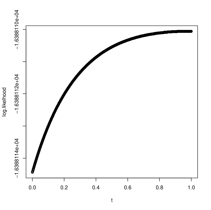
The behavior of the models for is similar. The log-likelihood values vary from () to () while the saturated log-likelihood is (see Figure 3, left). Table 2 gives the MLEs of the expected cell frequencies under the models , and . For we get , with -value .

Left Eye Grade
| Right Eye | ||||
|---|---|---|---|---|
| Grade | best | second | third | worst |
| best | 1520 | 266 | 124 | 66 |
| – | (263.38a/ 263.38b/ 263.39c) | (133.58/ 133.59/ 133.60) | (59.04/ 59.09/ 59.09) | |
| second | 234 | 1512 | 432 | 78 |
| (236.62/ 236.62/ 236.61) | – | (418.99/ 418.90/ 418.90) | (88.39/ 88.40/ 88.40) | |
| third | 117 | 362 | 1772 | 205 |
| (107.42/ 107.40/ 107.40) | (375.01/ 375.10/ 375.10) | – | (201.57/ 201.58/ 201.58) | |
| worst | 36 | 82 | 179 | 492 |
| (42.96/ 42.91/ 42.91) | (71.61/ 71.60/ 71.60) | (182.43/ 182.42/ 182.42) | – |
Examples for which the members of the family are not of similar performance are the two tables of Kateri and Papaioannou (1997, Tables 3 and 4), displayed in Table 3 (a) and (b).
|
|
|
Here, the models and differ considerably in their fit. In particular, the data in Table 3 (a) are modeled well by but not by ( and ), while the opposite holds for Table 3 (b), since and .
In such situations, the question arises whether some is appropriate for both data sets. Finding such that works for two or more tables of the same set-up is of special interest in the study of stratified tables. Using the same model on all strata makes parameter estimates among models comparable. This is a major advantage of the proposed family.
Models that lie ‘in-between’ the two extreme cases ( and ) may lead to a consensus. Even if that consensus model does not perform as well as and on each table separately, it can provide a reasonable fit for both tables. To visualize this, Figure 4 (left) shows the -values of the fit of the models with , for Tables 3 (a) and (b), by solid and dashed curves, respectively, along with the significance level of . The consensus model would have . Among these models, we propose , since the intersection of the two curves happens around . The fit of this model for Table 3 (a) is (-value=0.1314) while for (b) it is (-value=0.1409). The vector of MLEs for parameters is and , respectively. We note that, in deriving the consensus model, the values could have been used as an alternative to the -values in Figure 4.


 |
 |
 |
 |
In all examples treated so far, the log-likelihood under was monotone in (see Figure 3, left, and Figure 5, upper), suggesting that the ‘best’ model will be achieved at either or . This is not always the case. For example, for the data in Table 3 (c), the best fit occurs for (see also Figure 3, right), giving (-value=0.9989) while for and , it is (-value= 0.8049) and (-value=0.2914), respectively. Furthermore, even when the best model is for or , we may still want to use some , e.g. for stratified tables with different optimal model at each level of the stratifying variable, as explained above.
Applying the quasisymmetric independence models to Tables 3 (a) and (b), we observe that fits well on Table 3 (a) but not on (b), while model is of acceptable fit for both data sets. Indeed, we have (-value=0.8511), (-value=0.0184), (-value=0.1671) and (-value=0.2095). For the performance of the model for , see Figure 4 (right) and Figure 5 (lower). For , the -value of the fit of the model is equal to 0.1983 for both data sets.
All the examples of this section were worked out with R functions we developed for fitting the and models via the unidimensional Newton’s method. The adopted inferential approach is asymptotic. In cases of small sample size, exact inference can be carried out via algebraic computations along the lines described in Section 3, and demonstrated in Examples 4.1 and 4.2.
7 Divergence Measures
The one-parameter family of QS models we proposed, , , connects the classical QS model () and the Pearsonian QS model (). These two belong both to a broader class of generalized QS models that are derived using the concept of –divergence (Kateri and Papaioannou, 1997; Pardo, 2006). Measures of divergence quantify the distance between two probability distributions and play an important role in information theory and statistical inference. A well known divergence measure is the Kullback-Leibler (KL) divergence. However there exist broader classes of divergences. Such a class, including the KL as a special case, is the -divergence. In the framework of two-dimensional contingency tables, this class is defined as follows.
Let and be two discrete bivariate probability distributions. The –divergence between and (or Csiszar’s measure of information in about ) is defined by
| (33) |
Here is a convex function such that , , and . For and , the divergence (33) becomes the KL and the Pearson’s divergence, respectively. We adopt the notation in Pardo (2006). For properties of -divergence, as well as a list of well-known divergences belonging to this family, we refer to (Pardo, 2006, Section 1.2). The differential geometric structure of the Riemannian metric induced by such a divergence function is studied by Amari and Cichocki (2010).
The generalized QS models introduced by Kateri and Papaioannou (1997) are based on the -divergence and are characterized by the fact that each model in this class is the closest model to symmetry S, when the distance is measured by the corresponding divergence measure. The classical QS model corresponds to the KL divergence, while the Pearsonian QS corresponds to Pearson’s distance. We shall prove in Theorem 7.1 that the other members of the family, i.e. for , are -divergence QS models as well, and we identify the corresponding function.
Theorem 7.1.
Proof.
We set , where is just a constant for given . This choice of constant ensures . Then the inverse function to is
With this, we can write
where
We next rewrite as
Setting and , this translates into our parametrization (4). Now the result follows from Kateri and Papaioannou (1997, Theorem 1). For a probability table with symmetry S, the quantity is minimized when is the probability table satisfying . ∎
The fact that the models are -divergence QS models implies that they share all the desirable properties of the -divergence QS models (Kateri and Papaioannou, 1997). This includes the properties that highlight the physical interpretation issues of these models. As far as we know, the -divergence for the parametric function (34) has not been considered so far. Its study can be the subject of further research. Such a future project has the potential to build a bridge between information geometry (Amari and Cichocki, 2010) and algebraic statistics (Drton et al., 2009).
Acknowledgements.
Fatemeh Mohammadi was supported by the Alexander von Humboldt Foundation.
Bernd Sturmfels was supported by the NSF (DMS-0968882) and DARPA (HR0011-12-1-0011).
References
- Amari and Cichocki (2010) Amari, S. & Cichocki, A. (2010). Information geometry of divergence functions. Bulletin of the Polish Academy of Sciences, Technical Sciences 58, 183–195.
- Bishop et al. (1975) Bishop, Y.M.M., Fienberg, S.E. & Holland, P.W. (1975). Discrete Multivariate Analysis: Theory and Practice, MIT Press, Cambridge, Mass.
- Bowker (1948) Bowker, A.H. (1948). A test for symmetry in contingency tables. Journal of the American Statistical Association 43, 572–574.
- Caussinus (1965) Caussinus, H. (1965). Contribution l’ analyse statistique des tableaux de corrlation. Ann. Fac. Sci. Univ. Toulouse 29, 77–182.
- Drton et al. (2009) Drton, M., Sturmfels, B. & Sullivant, S. (2009). Lectures on Algebraic Statistics, Oberwolfach Seminars, Vol 39, Birkhäuser, Basel.
- Kateri and Agresti (2010) Kateri, M. & Agresti, A. (2010). A generalized regression model for a binary response. Statistics and Probability Letters 80, 89–95.
- Kateri and Papaioannou (1997) Kateri, M. & Papaioannou, T. (1997). Asymmetry models for contingency tables. Journal of the American Statistical Association 92, 1124–1131.
- Miller and Sturmfels (2005) Miller, E. & Sturmfels, B. (2005). Combinatorial Commutative Algebra, Graduate Texts in Mathematics, 227, Springer-Verlag, New York.
- Pachter and Sturmfels (2005) Pachter, L. & Sturmfels, B. (2005). Algebraic Statistics for Computational Biology, Cambridge University Press.
- Pardo (2006) Pardo, L. (2006). Statistical Inference Based on Divergence Measures, Chapman & Hall, Boca Raton, FL.
- Rapallo (2003) Rapallo, F. (2003). Algebraic Markov bases and MCMC for contingency tables. Scandinavian Journal of Statistics 30, 385–397.
- Stuart (1953) Stuart, A. (1953). The estimation and computation of strengths of association in contingency tables. Biometrika 40, 105–110.
- Sturmfels (1996) Sturmfels, B. (1996). Gröbner Bases and Convex Polytopes, University Lecture Series, vol. 8, American Mathematical Society, Providence, RI.
Authors’ addresses:
Maria Kateri, Institute of Statistics, RWTH Aachen University, 52056 Aachen, Germany,
kateri@stochastik.rwth-aachen.de
Fatemeh Mohammadi, Institut für Mathematik, Universität Osnabrück, 49069 Osnabrück,
Germany, fatemeh.mohammadi716@gmail.com
Bernd Sturmfels, University of California, Berkeley, CA 94720, USA, bernd@berkeley.edu