Origin of band gaps in graphene on hexagonal boron nitride
Abstract
Recent progress in preparing well controlled 2D van der Waals heterojunctions has opened up a new frontier in materials physics. In this paper we address the intriguing energy gaps that are sometimes observed when a graphene sheet is placed on a hexagonal boron nitride substrate, demonstrating that they are produced by an interesting interplay between structural and electronic properties, including electronic many-body exchange interactions. Our theory is able to explain the observed gap behavior by accounting first for the structural relaxation of graphene’s carbon atoms when placed on a boron nitride substrate and then for the influence of the substrate on low-energy -electrons located at relaxed carbon atom sites. The methods we employ can be applied to many other van der Waals heterojunctions.
pacs
73.22.Pr, 71.20.GjI Introduction
Recent progress in preparing vertical heterojunctions of graphene (G) and hexagonal boron nitride (BN) using either transfer [1] or growth techniques [2] has opened a new frontier for exploring both fundamental physics [3, 5, 4] and new device geometries [6]. Experiments have made it clear that graphene on BN is very flat and that its low-energy electronic states are often very weakly perturbed by the substrate [1]. However when the honeycomb lattices of graphene and BN are close to orientational alignment, the electronic coupling strengthens and is readily observed [7]. The source of this variability in behavior is clearly related to variability in structure. For example, although ab initio theory [8, 9] predicts substantial gaps meV when the two honeycomb lattices are identical, any incommensurability due to misorientation or lattice constant mismatch drastically reduces electronic coupling giving vanishingly small gaps [10]. In this article we show that the large gaps observed [3] at the Fermi level of neutral graphene sheets that are nearly rotationally aligned with a BN substrate are not due solely in terms of the relative orientation-dependent moiré pattern, but require in addition both orientation-dependent structural relaxation of the carbon atoms, as suggested by recent experiments [11], and non-local many-body exchange interactions between electrons. Our theory involves two elements: i) structural relaxation due to interactions between G and the BN substrate and ii) an effective Hamiltonian for graphene’s -electrons which includes a substrate interaction term that is dependent on the local coordination between graphene and BN honeycombs. Our main results are summarized in Fig. 1 where we show that atomic relaxation leads to substantially enhanced gap. The band gap for rotationally aligned layers is only meV when the honeycomb lattices are held rigid, but increases to 7 meV when relaxation is allowed. These gaps are further enhanced to meV, in reasonable agreement with experiment, when we also account for electron-electron interactions. Moreover, unlike other proposed mechanisms for band gaps in graphene [12], ours does not degrade the mobility of graphene.
II Moiré patterns and strains
The -electron Hamiltonian of G/BN can be expressed as the sum of the continuum model Dirac Hamiltonian of an isolated flat graphene sheet, in which the honeycomb sublattice degree-of-freedom appears as a pseudo spin, and a correction from the interaction with the BN substrate [7, 9, 10, 13]. We employ an approach in which the correction is given by a sub-lattice dependent but spatially local operator derived from ab initio theory [9] that depends on the local alignment between G and BN honeycomb lattices . This pseudo-spin dependent operator that gives rise to the moiré superlattice Hamiltonian is accurately parameterized in Ref. [9]. (An alternate parameterization which allows spatial variation in the interlayer separation is discussed in the appendix.)
When both G and BN form rigid honeycomb lattices
| (1) |
where is the difference between their lattice constants, is the difference in their orientations, and is the direction normal to the G sheet. The two layers establish a moiré pattern in which equivalent alignments repeat periodically on a length scale that, when and are small, is long compared to the honeycomb lattice constant. (The moiré lattice vectors solve where is a honeycomb lattice vector.) Since , the substrate interaction Hamiltonian has the periodicity of the moiré pattern.
When the honeycomb lattices of the G and BN layers are allowed to relax, is no longer a simple linear function of position. We write
| (2) |
where is the mean separation between G and BN planes and the in-plane and vertical strains, and , also have the moiré pattern periodicity. If G/BN systems achieved thermal equilibrium , , and would be determined by minimizing free energy with respect to the positions of atoms in the G layer and in the BN layers close to the surface of the substrate. Evidently this is not the case since the observed value of varies in an irreproducible fashion. In the following we take the view that because the thermodynamic bias favoring a particular value of is weak, its observed value is fixed by transfer kinetics. Similarly the value of , which can be adjusted only by atomic rearrangements on long length scales, is also likely determined by kinetics and not by equilibrium considerations. On the other hand, given values for and minimizing energy with respect to local strains and require only local atomic arrangements. We therefore view and as experimentally measurable system parameters. In practice is close to the undisturbed relative lattice constant difference whereas varies widely. The ratio of the honeycomb lattice constant to the moiré pattern lattice constant is . For given values of and , is dependent on strains because of their contribution to Eq. 2. The strains must therefore be calculated first in order to fix the -dependent -band Hamiltonian of G/BN. As a side remark, we note that is a convenient approximation for the coordination vector that can account for the twist angle dependence through the magnitude of but ignores the variations in the shape of the moire pattern.
Like the -electron Hamiltonian, the graphene sheet energy can be written as the sum of an isolated G layer contribution and a substrate interaction contribution that depends on the local band alignment . The substrate interaction is most attractive when half the carbon atoms are directly above boron atoms, and the centers of graphene’s hexagonal plaquettes are directly above the nitrogen atoms (BA alignment). This alignment is energetically more stable than one in which half the carbon atoms sit on top of nitrogen (AB alignment), or one in which all carbon atoms sit on top of either boron and nitrogen atoms (AA stacking). By performing ab initio calculations for commensurate lattices we find that . The full dependence of on is plotted in Fig. 2.

When or are non-zero, the substrate interaction forces plotted in Fig. 2 drive strains which attempt to match G and BN lattice constants locally and increase the sample area that is close to local BA coordination. For a given value of , G sheet lattice constant expansion near BA points must be compensated by lattice compression elsewhere. This kind of local expansion and compression of the graphene lattice within the moiré unit cell was recently identified experimentally [11, 14].
We determine the strains by minimizing the sum of the isolated graphene and substrate interaction energies. For the long-period moiré lattices the graphene sheet energy is accurately parameterized in terms of its elastic constants. The competition between isolated graphene and substrate interaction energies can then be understood by comparing the energies of the configurations in which the two terms are minimized separately. The substrate interaction energy is minimized by maintaining perfect BA alignment everywhere and therefore establishing commensurability between the BN and G lattices. Because the lattice constants of BN and G differ, this arrangement has an elastic energy cost in the graphene sheet. After an elementary calculation we find that the total energy per area is
| (3) |
where and are elastic constants, is the relative difference between BN and G lattice constants, and is the unit cell area of graphene. The elastic energy, on the other hand, is minimized by keeping the graphene sheet lattice constant at its isolated value. In this configuration, because of the linear relationship between and the substrate interaction energy per unit area is equal to the average of over :
| (4) |
As indicated in Fig. 1, when our theoretical values for are combined with the elastic constants of a graphene sheet, the energy of the commensurate state is substantially lower. However, Eq. (3) overestimates the elastic energy cost of lattice matching between BN and G. For example in the extreme case of a single BN layer, lattice matching can be achieved by adjusting the lattice constants of each layer toward their mean value, approximately reducing the required strains by a factor of 2. In this case, the incommensurate structure still has lower energy, but the difference is smaller. We conclude that when they are orientationally aligned, the interaction between a G sheet and a BN sheet is nearly strong enough to favor lattice matching.
G/BN is close enough to an incommensurate to commensurate transition that substantial strains can be driven by substrate interactions. Indeed we find by explicit energy minimization that both vertical and horizontal strains can assume values large enough to introduce changes in the electronic structure. We determined these strains numerically for the case of a single-layer BN substrate subject to a fixed periodic potential created by the layers underneath using methods explained in the appendix. We find that strains in the graphene sheet are comparable as those in the BN layer. Note that the atomic structure, and hence the -band Hamiltonian, might therefore depend on the thickness of the BN and on other features that vary from one experimental study to another. Similarly the addition of encapsulating layers can lead to reductions in strains and hence gaps, as recently reported in Ref. [11], although the gap can in principle persist.
III Strained moiré band Hamiltonian
Given and , we obtain a sublattice-pseudospin dependent continuum Hamiltonian with the periodicity of the moiré pattern which is conveniently analyzed using a plane-wave expansion approach. We write the full Hamiltonian in the form
| (5) | |||||
where is the Dirac Hamiltonian and is the Fourier transform over one period of the moiré pattern of , and is a moiré pattern reciprocal lattice vector. In Eq. (5), when is a moiré pattern reciprocal lattice vector and zero otherwise.
The electronic structures implied by the Hamiltonian in Eq. (5) for rigid lattices, for graphene relaxation only, and for mutual G and BN relaxation are compared in Fig. (3). These results demonstrate that the electronic structure, and the gap at neutrality in particular, depend sensitively not only on and but also on the strains. Sizable band gaps appear at the neutral system Fermi level only when in-plane relaxation strains are allowed.

IV Physics of the Gaps
Several potential mechanisms of gap formation in neutral graphene have been discussed in the literature including antidots [15], combinations of periodic scalar and vector fields [16, 17], and zero-line localization [18]. Our approach allows for a simple classification based on the Fourier expansion of . We will discuss leading contributions to the gap at neutrality in terms of the expansion of each moiré pattern Fourier component of into four sublattice Pauli matrix components. We start with the Fourier component, i.e with the spatial average of . In the absence of relaxation, because the average of is zero [9] and in this case is a linear function of . (We neglect an irrelevant contribution proportional to the identity sublattice Pauli matrix .) When is a non-linear function of , however, the spatial average of Hamiltonian contributions which are sinusoidal functions of do not vanish. Among these, the term proportional to is an irrelevant constant, and the terms proportional to and , often interpreted in Dirac models as effective vector potentials, simply shift band crossings away from zero momentum. (In the continuum Dirac model of graphene, momentum is measured away from the Brillouin-zone corners.) However, the term proportional to produces a gap
| (6) |
Physically this gap appears simply because the average site energy is different on different honeycomb sublattices.
The leading contributions to the gap from terms in are more subtle and appear at second order in perturbation theory. A perturbative treatment is in fact valid in practice because it turns out that is substantially larger than . Applying degenerate state perturbation theory we obtain the following expression for their contribution to the effective sublattice Hamiltonian at the Dirac point:
| (7) |
where ( is the Dirac velocity and is the vector of Pauli matrices,) ignoring the dependence close to the Dirac point which will be higher order. Note that connects the and blocks of the plane-wave expansion moiré band Hamiltonian. Because only the term proportional to can produce a gap at 2nd order, it is instructive to decompose into Pauli matrix contributions.
| (8) |
Note that higher order terms proportional to and may in principle contribute to the gap, but we find them to be negligible. We have derived analytic expressions for in terms of the Pauli matrix decomposition of which are discussed in detail in the appendix. We find that although the contribution to the gap is always larger, the contributions are not negligible. Both the difference in the spatial average of sub band energies and the detailed form of the full substrate interaction Hamiltonian play a role in determining the size of the gap at neutrality, and both are sensitive to the detailed structure of the lattice relaxation strains.
In graphene non-local exchange interactions are expected to enhance gaps [21, 23, 22] at neutrality produced by sublattice-dependent potentials. We have performed plane-wave-expansion self-consistent Hartree-Fock calculations in which Coulomb interactions are added to the moiré band Hamiltonian we have discussed. The calculations were performed using effective dielectric constants bracketing the expected values between and . When all effects are included we find band gaps meV, as shown in the inset of Fig. 1. The values chosen for partly account for dielectric screening by the substrate and partly accounts for dynamic screening effects in the same spirit as in the screened exchange functionals used in density-functional theory. We have previously used a similar dielectric constant of to successfully predict spontaneous band gaps meV in ABC trilayer graphene [24]. Further details of the Hartree-Fock theory in moire superlattice bands will be presented elsewhere [25].
V Discussion
We have derived a -band continuum model Hamiltonian intended to describe states near the Fermi level of G/BN and used it to address the energy gaps often observed in neutral graphene when it is nearly aligned with a BN substrate. In this theory the interaction of -band electrons with the substrate is described by a local but sublattice dependent term that is dependent on the local relative displacement of the graphene sheet and substrate honeycomb lattices, . When neither the G sheet’s carbon atoms nor the boron and nitrogen atoms in the substrate are allowed to relax, is a linear function of position because of the difference between the lattice constants and because of difference in orientations specified by a relative angle . The gap produced by substrate interactions in the absence of relaxation reaches its maximum at , but is never larger than a few meV and too small to explain experimental observations. Only by allowing the carbon and substrate atoms to relax we can explain the much larger experimental gaps.
The moiré pattern formed by graphene and a BN substrate is characterized in the first place by the lattice constant difference and by the relative orientation angle . These two quantities can be changed only by collective motion of many atoms. We take the view that because of large barriers and weak thermodynamic drivers these two macroscopic variables are not in practice relaxed to equilibrium values. We therefore view them as observables that characterize particular G/BN systems and calculate relaxation strains and -band electronic structure as a function of and , and hence as a function of moiré pattern period. The explicit calculations reported on in this paper are for , the orientation which leads to large experimental gaps.
To account for relaxation strains, we minimize the total energy with respect to carbon and substrate atom positions. For this purpose we assume that the interaction energy between graphene and substrate is also a local function of and obtain from density functional calculations of commensurate structures. The strains minimize the total energy by increasing the number of carbon atoms that are on top of boron atoms and the number of hexagonal carbon atom plaquettes that are centered above nitrogen atoms. Our study emphasizes that atom relaxation in the BN sheets is as important for the electronic structure as atom relaxation in the graphene sheet. Although only atom positions in the top BN sheet are important for electronic structure, these will be affected by interactions with atoms in remote layers. We have performed calculations for two extreme cases, rigid BN atoms and a single-layer of BN in which atom positions relax to minimize total energy, finding that relaxation increases the energy gap substantially. The physical origin of these gaps can be revealed by expanding the continuum model -band Hamiltonian in terms of Pauli-matrix pseudospin operators and in terms of moiré pattern reciprocal lattice vector components. Because of the wide -band width and the relatively short moiré periods, the contribution of each term in the Hamiltonian to the gap can be analyzed using leading order perturbation theory. The terms which capture detailed spatial patterns contribute at second order and are not negligible. The largest contribution to the gap comes from the term, which vanishes in the absence of lattice relaxation has a very simple interpretation. Because of relaxation strains the average site energy in the carbon sheet is different for the two carbon atom sub lattices. It is well known that this type of perturbation produces a gap at the Fermi level of a neutral graphene sheet. Surprisingly the gap is a substantial fraction of the gap of the same origin present in the commensurate BA aligned graphene on BN. The gaps are therefore due to the contrast between the local classical physics of energy minimization with respect to atom position, and the wide -bands and non-local quantum physics which forces the quantum wave functions to be smooth and sensitive mainly to spatial averages over the moiré period. When many-body interaction effects [21] are accounted for, these gaps are enhanced to values that are consistent with experiment. The approach described in this paper can be applied to other van der Waals materials which can form heterojunctions in which different layers have slightly different lattice constants or differ in orientation - such as transition metal dichalcogenide stacks.
VI Methods
The elastic energy functional was modeled using the Born-von Karman plate theory [27]. Neglecting the small bending rigidity of graphene eV [28] the elasticity theory depends on the two Lamé parameters whose estimates for graphene from empirical potentials gives eV/ and eV/ [29] in the low temperature limit, and for a single BN sheet we have used and [26] obtained averaging the LDA and GGA values. The potential energy has been parametrized from the stacking-dependent and separation dependent energy curves in Ref. [26] calculated at the EXX+RPA level. The scalar functions used to obtain the moiré superlattice pattern for the height and the displacement vectors from their gradients have used written as a Fourier expansion in vectors as
| (9) | |||||
where is in general a complex number and we retain up to three nearest vectors for the scalar field that preserves the symmetry of triangular lattices. The parameters , , , , and are real valued constants and we defined auxiliary functions and in terms of the triangular lattice structure factors similar as those used in a general tight-binding model of graphene [30]. The Fourier expansion coefficients within the first shell consisting of and the first shell are often good representation of the solutions. Further details on the calculation method and results of the elastostatic problem can be found in the appendix. The self-consistency Hartree-Fock calculations were calculated using an effective relative dielectric constant of using 217 -points in the moiré Brillouin zone.
VII Acknowledgments
The work in Singapore was supported by National Research Foundation of Singapore under its Fellowship program (NRF-NRFF2012-01). The work in Austin was supported by the Department of Energy, Office of Basic Energy Sciences under contract DE-FG02-ER45118, and by the Welch Foundation grant TBF1473. We acknowledge use of computational resources from the Texas Advanced Computing Center and the high performance computing center at the Graphene Research Centre at the National University of Singapore. We acknowledge helpful discussions with Andre Geim and Gareth Jones and the assistance from Miguel Dias Costa for troubleshooting the parallel implementation of the Hartree-Fock calculations.
VIII Author contributions
JJ and AMD executed research. All authors contributed in conceiving, discussing and preparing the manuscript.
IX Conflicts in financial interest
The authors declare no conflicting financial interests.
References
- [1] Dean, C. R. et al. Boron nitride substrates for high-quality graphene electronics. Nature Nanotechnology 5, 722–726 (2010).
- [2] Yang, W. et al. Epitaxial growth of single-domain graphene on hexagonal boron nitride . Nature Materials 12, 792–797 (2013).
- [3] Hunt, B. et al. Massive dirac fermions and hofstadter butterfly in a van der waals heterostructure. Science 340, 1427–1430 (2013).
- [4] Ponomarenko, L. A. et al. Cloning of dirac fermions in graphene superlattices. Nature 497, 594–597 (2013).
- [5] Dean, C. R. et al. Hofstadter’s butterfly and the fractal quantum hall effect in moiré superlattices. Nature 497, 598–602 (2013).
- [6] Britnell, L. et al. Field-Effect Tunneling Transistor Based on Vertical Graphene Heterostructures. Science 335, 947–950 (2012).
- [7] Yankowitz, M. et al. Emergence of superlattice dirac points in graphene on hexagonal boron nitride. Nature Physics 8, 382–386 (2012).
- [8] Giovannetti, G., Khomyakov, P. A., Brocks, G., Kelly, P. J. & van den Brink, J. Substrate-induced band gap in graphene on hexagonal boron nitride: Ab initio density functional calculations. Physical Review B 76, 073103 (2007).
- [9] Jung, J., Raoux, A., Qiao, Z. & MacDonald, A. H. Ab-initio theory of moiré superlattice bands in layered two-dimensional materials. Physical Review B 89, 205414 (2014).
- [10] Ortix, C., Yang, L., van den Brink, J. Graphene on incommensurate substrates: Trigonal warping and emerging Dirac cone replicas with halved group velocity. Physical Review B [cond-mat] 86, 081405 (2012).
- [11] Woods, C. R. et al. Commensurate-incommensurate transition for graphene on hexagonal boron nitride. Nature Physics, DOI:10.1038/nphys2954 (2014).
- [12] Novoselov, K. Graphene: Mind the gap. Nature Materials 6, 720–721 (2007).
- [13] Wallbank, J. R., Patel, A. A., Mucha-Kruczyński, M., Geim, A. K. & Fal’ko, V. I. Generic miniband structure of graphene on a hexagonal substrate. Physical Review B 87, 245408 (2013).
- [14] Tang, S. et al. Precisely aligned graphene grown on hexagonal boron nitride by catalyst free chemical vapor deposition. Scientific Reports 3 (2013).
- [15] Pedersen, T. G. et al. Graphene antidot lattices: Designed defects and spin qubits. Physical Review Letters 100, 136804 (2008).
- [16] Snyman, I. Gapped state of a carbon monolayer in periodic magnetic and electric fields. Physical Review B 80, 054303 (2009).
- [17] Low, T., Guinea, F. & Katsnelson, M. I. Gaps tunable by electrostatic gates in strained graphene. Physical Review B 83, 195436 (2011).
- [18] Kindermann, M., Uchoa, B. & Miller, D. L. Zero-energy modes and gate-tunable gap in graphene on hexagonal boron nitride. Physical Review B 86, 115415 (2012).
- [19] Bistritzer, R. & MacDonald, A. H. Moiré bands in twisted double-layer graphene. Proceedings of the National Academy of Sciences 108, 12233–12237 (2011).
- [20] Vozmediano, M., Katsnelson, M. & Guinea, F. Gauge fields in graphene. Physics Reports 496, 109–148 (2010).
- [21] MacDonald, A. H. , Jung, J., Zhang, F., Pseudospin Order in Monolayer, Bilayer, and Double-Layer Graphene. Phys. Scr. 014012 (2012).
- [22] Bokdam M. Amlaki T. Kelly P. J. Band gaps in incommensurable graphene on hexagonal boron nitride, Physical Review B 89 201404(R) (2014).
- [23] Song, J. C. W., Shytov, A. V., and Levitov, L. S., Electron interactions and gap opening in graphene superlattices, Physical Review Letters 111, 266801 (2013).
- [24] Jung J., and MacDonald, A. H. Gapped broken symmetry states in ABC-stacked trilayer graphene, Physical Review B 88, 075408 (2013).
- [25] DaSilva A. M. et al. unpublished.
- [26] Sachs, B., Wehling, T. O., Katsnelson, M. I. & Lichtenstein, A. I. Adhesion and electronic structure of graphene on hexagonal boron nitride substrates. Physical Review B 84, 195414 (2011).
- [27] Washizu, K. Variational methods in elasticity and plasticity (Pergamon Press, 1975).
- [28] Koskinen, P. & Kit, O. O. Approximate modeling of spherical membranes. Physical Review B 82, 235420 (2010).
- [29] Zakharchenko, K. V., Katsnelson, M. I. & Fasolino, A. Finite temperature lattice properties of graphene beyond the quasiharmonic approximation. Physical Review Letters 102, 046808 (2009).
- [30] Jung, J., MacDonald, A. H. Tight-binding model for graphene -bands from maximally localized Wannier functions, Physical Review B 87 195450 (2013).
Appendix.
In the following we supplement the information in the main text introducing: the parametrization of the Hamiltonian in real-space, the explicit form of the scalar fields with the moiré superlattice symmetry, the elastic energy functionals, the parametrization of the potential energy, the formulation and solutions to the elastostatic problem for the relaxed ground states, and the contributions of the different pseudospin terms in the Hamiltonian to the primary Dirac point band gap, both numerically and analytically through second-order perturbation theory.
Appendix A Parametrization of the Hamiltonian
The diagonal and off-diagonal elements of the Hamiltonian for a fixed interlayer separation distance can be written in the sublattice basis in a manner similar to the pseudospin representation used in Ref. [1],
| (10) | |||||
The out-of-plane -axis layer separation dependence can be incorporated into the three main coefficients with an exponentially decaying behavior in the form
| (11) |
where , and the three decay coefficients for each one of the terms of the Hamiltonian in the sublattice basis were found fitting the -dependence between 2.8 to 5 , where we use the parameters obtained from ab initio calculations
| (12) | |||||
| (13) | |||||
| (14) |
whose equivalent values in the pseudospin basis had been calculated previously [1]. The variation of the phase with shows a weak linear dependence and we can approximate it as a constant value. The effects due to lattice relaxation can be conveniently incorporated when calculating the Fourier expansion of the above Hamiltonian by accounting for the in-plane displacement in the stacking coordination vector , as explained in the main text, and the height that represents the local distance of graphene to BN, where is a two-dimensional vector. Both the displacement vectors and the height maps are assumed to respect the moiré periodicity and are therefore modeled from the scalar fields that we introduce in the following section.
Appendix B Scalar fields for describing the moiré patterns
In the main text we presented an approximation for a scalar field that varies smoothly in real space that respects the symmetry of the triangular superlattice to use in the variational trial functions. For brevity in notation here we use to indicate the . The specific form of the trial functions we use are given by
| (15) | |||||
where the constants are complex numbers. The function
| (16) |
is defined in terms of the structure factors
| (17) | |||||
where , where is the real-space periodicity of the moiré superlattice and . These are momentum space analogues of the real space inter-sublattice hopping structure factors in a honeycomb lattice [2]. The explicit form of the functions defined along the symmetry lines or can be obtained from sums of
| (18) | |||||
The analytical expression for the function shell contribution reduces to a simpler form
| (19) |
where , that for the symmetry lines reduce to
| (20) |
The vector fields such as in-plane forces, displacement vectors, and stresses can be obtained as gradients of the scalar potentials given by the above forms that can preserve the symmetry of the triangular moiré superlattice. The vector field that can be obtained from the gradient of the scalar field is
| (21) |
and can be obtained taking the respective partial derivatives. Thus we have
| (22) |
where the partial derivatives of the constituent functions are given by
| (23) | |||||
For the terms we have
| (24) |
Likewise higher order derivatives used in the stress tensors or the gauge fields can be evaluated analytically. The pair of parameters and for each function and the single parameter accompanying the function specify the variational space we used to minimize the energy functionals. Because the term captures the first harmonic contribution, the different variables such as , , can be characterized in terms of just two parameters and , or up to three when the average value of the origin is required.
Appendix C Elastic and potential energy functionals
C.1 Elastic energy functional
The elastic energy for the Born-von Karman plate theory can be obtained in terms of the Lamé parameters since the small bending stiffness for graphene or BN plays a negligible role [3]. For graphene we use , valid close to zero 0 K have been estimated from empirical potentials [4] and the for a single sheet of BN use the DFT estimates , obtained averaging the LDA and GGA values. The total elastic energy per superlattice area is given by [5, 6]
| (25) | |||||
The strain tensors associated to the deformation of the graphene layer depend both on the in-plane displacements and heights in Monge’s representation:
| (26) | |||||
In a practical calculation it is convenient to use an integration domain that remains fixed for every moiré period. For this purpose we use rescaled coordinates to operate in the coordination vector defined in the unit cell of graphene. Using the chain rule to relate the reduced vector in graphene’s unit cell and the real-space coordinates for zero twist angle and assuming variable lattice constant mismatch we have
| (27) |
When we neglect the contributions from the height variation the elastic energy can be written as
| (28) |
where represents the integrand of Eq. (28) in rescaled coordinates . This form shows more explicitly a weakening of the elastic energy as the lattice constant mismatch becomes smaller.
C.2 Parametrization of the potential energy
Likewise it is convenient to use the parametrization of the potential energy in the coordination vector and the interlayer separation height. The potential energy term has been parametrized from EXX+RPA calculations binding energy curves for different stacking configurations [7] as a starting point to extract the potential energy curves needed for the formulation of the Frenkel-Kontorova (FK) model for this two-dimensional bipartite lattice. We can neglect the van der Waals tail corrections from the bulk that bring the equilibrium distances closer because their influence in distinguishing different stacking energies are small. We make use of the property that the energy landscape for a fixed -axis separation is given by a simple expansion in the first shell of G-vectors in Fourier space [1] to represent the energy map with three parameters. As noted previously the simplest approximation for a scalar field that varies smoothly in real space with the triangular lattice symmetry is given by
where the constants are complex numbers. Thanks to this simple form it is possible to parametrize the whole energy landscape from the values of the potentials at three inequivalent stacking configurations, for example the three symmetric stacking configurations AA, AB and BA. Its explicit expression
| (29) | |||||
repeats with the periodicity of a triangular lattice. The scalar function at the three distinct symmetry points in units of graphene’s lattice constant
| (30) | |||||
| (31) | |||||
| (32) | |||||
These equations lead to the explicit values of the parameters
| (33) | |||||
| (34) | |||||
| (35) |
where we have used the relation . From the layer separation -dependence of these three coefficients , and we can obtain the complete potential landscape that we need for our model. We note that the term is the average value of in the periodic domain for every value of and that the remaining and terms accounts for the landscape of the energy in the first harmonic approximation, which is often an accurate approximation for functions varying smoothly with the moiré pattern [1]. The difference between this average and the minimum gives a measure of the in-plane forces associated to the energy gradient in a Frenkel-Kontorova problem [8]. The numerical values for , and for the binding energy curves as a function of separation distance can be obtained from the calculations provided in Ref. [7]. They can be interpolated numerically or alternatively we can use analytic fitting expressions similar to that in Ref. [9] used in the G/G case. We define the auxiliary functions
| (36) | |||||
| (37) | |||||
| (38) |
with the parameters , , , , to define the fitting function for the average value of for all the stacking configurations through
| (39) | |||||
| (40) |
where is given in angstroms. We used a rather simple model for which is fairly accurate but can still be improved through additional parameters to better capture the behavior away from the equilibrium point. The -dependence of the term is easily captured through an exponentially decaying form
| (41) |
where , and , is the lattice constant of graphene. The term shows a weak linear dependence with respect to so we use a constant value. When necessary, the long-ranged van der Waals tails originating from the bulk BN layers can be added through
| (42) |
where is the separation lattice constant between the layers and whose sum saturates quickly. However, this correction term has a small influence for the differences in energy for different stacking arrangements and we neglect this term. The energy landscape plots for a fixed separation distance presented in Fig. 5
allows to estimate the average in-plane traction force being applied on the two inequivalent carbon atoms in the unit cell. Even though the LDA binding energies are substantially smaller than in an EXX+RPA calculation, we find that this in-plane energy map obtained through parametrization in Fig. 3 of the main text is closely similar to the LDA energy map obtained in Ref. [1], whose agreement is attributable to the dominance of short-range character of the interactions near equilibrium distances that is captured reasonably well by the LDA approximation [9].
From this potential landscape per two carbon atom unit cell we can infer the potential experienced by the individual carbon atoms that can be useful for lattice force-field calculations where the higher energy optical modes are treated explicitly. This is done assuming that the total potential energy consists of the sum of the potentials experienced by each carbon atom which is separated by a distance
| (43) |
Solving the above equation we get
| (44) |
where and . Likewise if the long-range van der Waals tails are used they would need to be reduced to one half of its value. In Fig. 5 we show the potential energy repeated over several periods as well as the energy landscape seen by each carbon atom, derived assuming additivity in the total potential energy.
Appendix D Relaxation of the graphene and substrate atoms in the G/BN heterojunction
The relaxed geometries can be readily obtained minimizing the elastic and potential energy functionals using the trial functions that we introduced earlier. We distinguish two different scenarios in our elasticity problem. In the first case we solve for the elastostatic solutions where we relax the atoms of graphene subject to a periodic moiré potential of a rigid substrate. A second scenario allows the coupled relaxation of the BN substrate atoms. For simplicity we consider only the zero twist angle case and variable lattice constant mismatch .
D.1 Graphene relaxation only model
The resolution of the elastostatic problem of graphene subject to a superlattice potential requires the minimization of the total energy functional
| (45) |
where is given in Eq. (28) and the potential energy is given by the integral in the moire supercell of area of the potential energy kernel given in Eq. (29)
| (46) |
The stacking coordination vector is modeled as
| (47) |
assuming that the substrate produces a rigid periodic potential pattern. We use the gradients of the scalar field in Eq. (21) to model the displacement vectors . The local elastic and potential energy maps corresponding to the small and large strain limits are represented in Fig. 6.

D.2 Coupled relaxation of the BN lattice
Here we explore the influence in the elastic of energy of graphene when the BN atoms of the topmost layer in the substrate are allowed to relax in response to the stacking rearrangement of the graphene sheet. The coupled motion of the substrate atoms contribute in decreasing the total elastic energy of the graphene BN heterojunction because a smaller displacement in the graphene sheet is needed than if the substrate remains rigid. For solving the coupled G/BN elasticity problem we will assume that the topmost BN sheet is subject to a potential stemming from the graphene sheet itself and the BN layers underneath, assuming that the BN atoms below the topmost layer remain fixed. The potential energy for fixed interlayer separation of for G/BN and BN/NB along the direction of stacking arrangement vector is shown in Fig. 7. The interaction potential between the two topmost BN layers are defined by meV and through the funciton .

Even though the binding energies and forces predicted by the LDA typically underestimate the values obtained from higher level RPA calculations [11, 12, 13, 14] we assume that the energy landscape for different strackings We used LDA energies for BN/NB coupling as a function of sliding, assuming that their sliding energy maps are comparable to EXX+RPA as we found for the G/BN case. The total energy of G/BN/NB where both sheets are allowed to relax is given by the sum of the elastic and potential energies of graphene and the topmost BN sheet. The total potential energy term can be obtained from the interaction energies between the neighboring layers through
| (48) |
and can be calculated from the parametrized potential energies evaluating the integrals in the moiré supercell
| (49) | |||||
| (50) |
where the kernels are functionals of the local stacking coordination functions and that depend on the displacements relative to the neighboring layers
| (51) | |||||
| (52) |
We used explicit labels G/BN and BN/NB to distinguish the interaction potentials. For the graphene sheet the only relevant reference frame is the topmost BN layer whereas the latter interacts both with the graphene sheet and the BN layers underneath whose coordinates are assumed to remain fixed.

Appendix E Strains in relaxed ground-states
As noted earlier, the strained geometries can be characterized by the magnitude and phases that define the scalar fields in Eq. (15) and vector fields in Eq. (21) within a restricted variational space that preserves the triangular moiré periodicity dictated by the lattice constant mismatch and twist angle . The solutions for the strains in the graphene layer can be largely characterized by two parameters and whereas the height profiles require three , and for the additional average interlayer separation. For the topmost BN sheet we only consider in-plane strains assuming that its separation from the additional BN layer underneath takes a constant average value. Because the relative magnitudes of the elastic and potential energies scale with the lattice constant mismatch a correction in the potential profiles or the average value of the elasticity constants would have an overall effect of shifting the solutions in the abscissa. Within our approximation, the solutions are completely characterized by the -dependent values of the parameters that define the scalar field. In Fig. 9 we show the values of the relaxed solution parameters where only the graphene sheet is allowed to relax both in-plane and out of plane. We also show a comparison with the solutions where only in-plane relaxation is permitted and we fix the interlayer separation to a constant value.
When we consider the coupled graphene and BN layer relaxation we notice an interesting behavior where the largest strain magnitudes are for the topmost BN sheet rather than graphene itself. The results for the relaxed strains of the coupled G/BN/NB heterojunction where both graphene and the topomost BN layer are relaxed is shown in Fig. 8. This is possible thanks to a special total energy landscape with easy sliding path in BN [15]. The BN sheets in the crystal substrate follows an AA′ stacking order and for this stacking configuration they have a minimum energy sliding path when going from AA′ to AB′ with a small barrier of about 3 meV and even smaller total energy differences of about 1 meV within the LDA. A more elaborate GGA + vdW functional calculation [15] predicted similar barrier magnitudes but with the minimum of energy happening for the AB′ stacking configuration with a total energy lower by 1.5 meV. These minute differences are unimportant for the solutions we discuss.
Appendix F Band gaps and the Fourier components of the strained Hamiltonian
The Hamiltonian of graphene is modified in a G/BN heterojunction by moiré patterns [1] that can be described in a transparent manner when represented in a pseudospin basis. The different contributions consist of a site potential , the mass or sublattice staggering potential and an in-plane pseudospin inter-sublattice coherence term as shown in Fig. 10. The latter is closely related with a pseudomagnetic field derived from the straining of the graphene sheet represented in Fig. 11.


As mentioned in the main text and explained in more detail in Ref. [1] it is possible to obtain the full band structure from the Fourier components represented in the moiré reciprocal lattice vectors . The term that most directly influences the band gap comes from , in particular the contribution which is the average mass in the a moiré supercell. This term normally vanishes to zero in a rigid crystal [1] but here we showed that they generally average to a nonzero value in the presence of in-plane strains. Farther shell contributions in do also contribute to the band gap through higher order corrections. The contributions from the first shell in G-vectors through second order perturbation theory play the most relevant role. In Fig. 12 we show a comparison of the nonzero average mass term and the total band gap as a function of moiré period. It is noteworthy that when out of plane relaxations are absent the values of the band gaps are generally smaller and the relative cancellation between the average mass and the second order contributions from the first shell are more substantial. The pseudomagnetic field term from , due to the anisotropic strains generated by the coupling with the BN substrate, plays a minor role in configuring the band gap at the primary Dirac point as will be made clearer in the perturbative analysis.


The other two components of the Hamiltonian, potential fluctuations and in-plane pseudospin terms represented in Figs. (13, 14), also see modifications due to straining, typically acquiring contributions beyond the first shell in G-vectors with the most important contributions ranging up to three nearest neighbor hoppings, and their Fourier components having magnitudes in the order of 10 meV.

The pseudomagnetic term generated by the strains in the graphene sheet itself can in principle have a contribution comparable to the contribution due to the electron virtual hopping to and back from the BN sheet. Using the expressions for pseudomagnetic fields in graphene provided in Refs. [16, 17]
| (53) | |||||
| (54) |
and using a typical map of its magnitude in real space is shown in Fig. 11. We note that the pseudomagnetic vector potentials follow a moiré period scaling relation given by when represented in rescaled coordinates of the moiré superlattice , in turn defined by the parameters that determine the displacement vectors .
Appendix G Second order perturbation theory
Further insight on the contributions to the band gaps can be achieved from second order perturbation theory from the first shell approximation. We distinguish two scenarios, one for rigid unrelaxed lattices and another where strains are allowed to modify the stacking coordination. Formally it is possible to show that for rigid unrelaxed lattices the in-plane gives a zero contribution to the band gap to second order in perturbation theory. When in-plane strains are allowed, band gaps develop thanks primarily to a nonzero average mass and all three pseudospin components make a nonzero contribution to the gap to second order. Among these, in our calculations the in-plane pseudospin terms contribute to the gap with a smaller magnitude than the Fourier expansion of the mass terms .
G.1 Unrelaxed configuration
Here we discuss the effective 2x2 Hamiltonian obtained from perturbation theory around the Dirac point. Our initial Hamiltonian is a matrix, where is two times the number of Moiré reciprocal lattice vectors in the Fourier transform. Treating the diagonal blocks as the unperturbed Hamiltonian, second order degenerate perturbation theory gives an effective Hamiltonian for the low energy states,
| (55) |
where are the blocks in the Hamiltonian associated with the moiré vector , and connect the and blocks of the Hamiltonian. If we ignore for a moment the relaxation due to in-plane strains, the diagonal blocks are , which has an inverse . We can decompose both the effective Hamiltonian and the into terms proportional to Pauli matrices,
| (56) | ||||
| (57) |
Since is hermitian, the parameters must be real numbers. However, each block is not necessarily hermitian, so are complex numbers. Plugging in the decomposed forms, and restricting to just the nearest shell of reciprocal lattice vectors (we use the index for ), we get
| (58) | ||||
| (59) | ||||
| (60) | ||||
| (61) |
The sums in the above equations are restricted to due to the relation and the property of the corresponding matrices, . We will now prove that . The moiré Hamiltonian has the property and . Therefore . However, . Examining the above equations, we see that due to the symmetry properties of the Hamiltonian, and the gap for the unrelaxed configuration arises entirely from a mass term .
We have numerically calculated the low energy eigenvalues as a function of the parameters to verify the second order perturbation theory result and show which terms contribute at third order and higher. Our numerical calculations are performed by multiplying each of the by interpolation parameters which range from 0 to 1, thus keeping the same relationship (magnitude and phase) between the different terms while allowing us to see explicitly the power law behavior of the gap due to each term.
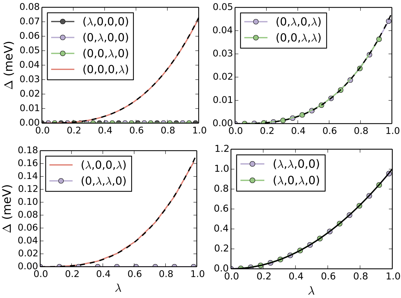
First we set all except for one. Power law fits show that there is no 2nd order contribution from any of the terms individually (Fig. 15). The term contributes at the 3rd order, while all others are 5th order or higher.
Next we look at the interplay between the different matrix elements which are found to contribute to the perturbation theory results for as described in the main text. Figure 15 confirm that to second order, the gap is not opened by terms proportional to , , , and . The first two, and do contribute to the energy levels at second order: they lead to a nonzero which does not open a gap. The term we found to be zero in the second order perturbation theory due to the symmetry of the Hamiltonian, which is verified here. Finally, the term does not appear in the second order perturbation theory at all, which is again confirmed by our numerical results. The only terms which contribute to the gap at second order, and are therefore most efficient at opening a gap, are and .
G.2 Relaxed configuration
We showed in the main text that the in-plane relaxation of the graphene and boron nitride lattices has a large effect on the size of the gap. This is due primarily to the emergence of nonzero mass in the block . This term alone slightly overestimates the gap. We again calculate a second order perturbation theory, Eqn. (55). However, it is no longer a good approximation to restrict to the nearest six reciprocal lattice vectors. This means that although the decompositions given in Equations (5861) remain valid, the symmetry properties that cause and to vanish do not strictly hold. We do, however, find that these terms are small. The primary contribution to the gap comes from the term which overshoots the gap. Including the second order terms produces an excellent approximation to the calculated gap. Thus we see explicitly that the relaxation is a key source of the gap opening in graphene/boron nitride bilayer systems.
References
- [1] Jung, J., Raoux, A., Qiao, Z. & MacDonald, A. H. Ab-initio theory of moire superlattice bands in layered two-dimensional materials. Physical Review B 89, 205414 (2014).
- [2] Jung, J. & MacDonald, A. H. Tight-binding model for graphene -bands from maximally localized wannier functions. Physical Review B 87, 195450 (2013).
- [3] Koskinen, P. & Kit, O. O. Approximate modeling of spherical membranes. Physical Review B 82, 235420 (2010).
- [4] Zakharchenko, K. V., Katsnelson, M. I. & Fasolino, A. Finite temperature lattice properties of graphene beyond the quasiharmonic approximation. Physical Review Letters 102, 046808 (2009).
- [5] Washizu, K. Variational methods in elasticity and plasticity (Pergamon Press, 1975).
- [6] Guinea, F., Horovitz, B. & Le Doussal, P. Gauge field induced by ripples in graphene. Physical Review B 77, 205421 (2008).
- [7] Sachs, B., Wehling, T. O., Katsnelson, M. I. & Lichtenstein, A. I. Adhesion and electronic structure of graphene on hexagonal boron nitride substrates. Physical Review B 84, 195414 (2011).
- [8] Braun, O. M. & Kivshar, Y. S. The Frenkel-Kontorova Model (Springer-Verlag, 2004).
- [9] Gould, T., Lebègue, S. & Dobson, J. F. Dispersion corrections in graphenic systems: a simple and effective model of binding. Journal of Physics: Condensed Matter 25, 445010 (2013).
- [10] Bull. Am. Phys. Soc. 59, 1 455 (2014). http://meetings.aps.org/link/BAPS.2014.MAR.F55.3
- [11] Jung, J., García-González, P., Dobson, J. F. & Godby, R. W. Effects beyond the random-phase approximation in calculating the interaction between metal films. Physical Review B 70, 205107 (2004).
- [12] Marini, A., García-González, P. & Rubio, A. First-principles description of correlation effects in layered materials. Physical Review Letters 96, 136404 (2006).
- [13] Lebègue, S. et al. Cohesive properties and asymptotics of the dispersion interaction in graphite by the random phase approximation. Physical Review Letters 105, 196401 (2010).
- [14] Björkman, T., Gulans, A., Krasheninnikov, A. V. & Nieminen, R. M. van der waals bonding in layered compounds from advanced density-functional first-principles calculations. Physical Review Letters 108, 235502 (2012).
- [15] Marom, N. et al. Stacking and registry effects in layered materials: The case of hexagonal boron nitride. Physical Review Letters 105, 046801 (2010).
- [16] Suzuura H. & Ando T. & Phonons and electron-phonon scattering in carbon nanotubes. Physical Review B 65, 235412 (2002).
- [17] Vozmediano, M., Katsnelson, M. & Guinea, F. Gauge fields in graphene. Physics Reports 496, 109–148 (2010).