Comparing disease control policies for interacting wild populations

Iulia Martina Bulai Roberto Cavoretto Bruna Chialva Davide Duma Ezio Venturino Affiliation: Department of Mathematics “Giuseppe Peano”, University of Torino, via Carlo Alberto 10, I–10123 Torino, Italy E-mail: iuliam@live.it Affiliation: Department of Mathematics “Giuseppe Peano”, University of Torino, via Carlo Alberto 10, I–10123 Torino, Italy E-mail: roberto.cavoretto@unito.it Affiliation: Department of Mathematics “Giuseppe Peano”, University of Torino, via Carlo Alberto 10, I–10123 Torino, Italy E-mail: bruna.chiara@alice.it Affiliation: Department of Mathematics “Giuseppe Peano”, University of Torino, via Carlo Alberto 10, I–10123 Torino, Italy E-mail: davideduma@gmail.com Affiliation: Department of Mathematics “Giuseppe Peano”, University of Torino, via Carlo Alberto 10, I–10123 Torino, Italy E-mail: ezio.venturino@unito.it

Abstract

We consider interacting population systems of predator-prey type, presenting four models of control strategies for epidemics among the prey. In particular to contain the transmissible disease, safety niches are considered, assuming they lessen the disease spread, but do not protect prey from predators. This represents a novelty with respect to standard ecosystems where the refuge prevents predators’ attacks. The niche is assumed either to protect the healthy individuals, or to hinder the infected ones to get in contact with the susceptibles, or finally to reduce altogether contacts that might lead to new cases of the infection. In addition a standard culling procedure is also analysed. The effectiveness of the different strategies are compared. Probably the environments providing a place where disease carriers cannot come in contact with the healthy individuals, or where their contact rates are lowered, seem to preferable for disease containment.

Keywords:

refuge niches culling disease transmission ecoepidemics

MSC

92D30 92D25 92D40

1 Introduction

In population models predator-prey and competition systems play a dominant role, since the blossoming of this discipline about a century ago. In more recent times, more refined models try to better describe reality. Since prey try to seek protection against attacks of their predators in the features of the environment, scientists have tried to incorporate this behavior into the interaction models. Early contributions in this respect can be found in [8, 4, 7]. The introduction of refuges has lead to the observation that the Lotka-Volterra models gets stabilized [3] even to show global asymptotic stability, [1, 2]. This shows the relevant role that spatial refuges exert in shaping the dynamics of predator-prey interplay. The refuge is expressed in the equations by reducing the amount of prey population available for hunting by the predators.

In this classical setting, if $Y$ denotes the prey population that can take cover, by $Y_{n}$ we denote the number of individuals who find protection in the niches that are available for their safety. Thus there are only $Y-Y_{n}$ individuals that can interact with the predators. There could be several functional forms that can be chosen for $Y_{n}$ . The simplest one is a constant value, $Y_{n}=Y_{0}$ , with $Y_{0}\in\textbf{R}_{+}$ , or alternatively one could take a linear function of the prey population, $Y_{n}=Y_{0}Y$ , [3] or also a linear function of the predators $X$ , $Y_{n}=Y_{0}X$ [9].

Ecoepidemiology investigates the influence of diseases in ecosystems, see Chapter 7 of [5]. It appears therefore that the refuges for some of the populations involved can be introduced also in this context. However, instead of using the environmental niches as protection against the predators, i.e. as an ecological tool as described above, we employ them in order to investigate whether they can influence the disease spread, i.e. we give them an epidemiological meaning. Therefore, it is not against predators that prey are protected, but we rather consider the case in which the healthy prey for some reason due to the conformation of the environment can avoid to come in contact with disease-carriers of their own population and therefore be somewhat protected from the epidemics. This is achieved by reduced contact rates that they have with infected individuals. Of all the various possible types of niche, to keep things simple, we just take the constant case, $Y_{n}=Y_{0}$ .

In the next Sections, we present three models for the refuges and one for another common disease-control method, namely culling, based on the ecoepidemic system presented in [10]. The first three differ in the way the refuge is modeled. In Section 2, some of the susceptibles are prevented from interaction with infected individuals. In Section 3, it is part of the infected that are unable to become in contact with healthy individuals. In Section 4, we look at a reduced contact rate. Section 5 contains the analysis of the culling strategy. After a brief discussion of bistability of some equilibria, the final Section compares the findings.

2 The refuge for the healthy prey

Consider at first the system in which the susceptibles are stronger and therefore able to reach places unattainable by the diseased individuals, because these indeed are weakened by the disease. Thus the infectious individuals cannot come in contact with the healthy remote individuals, and therefore cannot infect them. Let $s$ denote the fixed number of susceptibles that escape from the spread of the epidemics using the refuge.

The model is formulated as follows. The healthy prey $R$ reproduce with net reproduction rate $a$ , are subject to intraspecific competition only with other sound individuals at rate $b$ and are hunted by predators at rate $c$ . Those that can be infected by the diseased prey individuals $U$ , as discussed above, leave their class at rate $\lambda$ , to enter into the class of sick inviduals. The latter do not reproduce, are hunted at a rate $k\neq c$ by the predators. Here $k>c$ means that they are weaker than sound ones, and therefore easier to capture, while $k<c$ instead takes into account the fact that they might be less palatable than the healthy ones. Finally, they can recover the disease at rate $\omega$ and therefore reenter into the $R$ population. As mentioned above, infected are assumed not to contribute to intraspecific pressure, either of sound prey or among themselves; this again is grounded in the fact that their disease-related weakness prevents them to compete with the other individuals in the population. The predators are assumed to have also other food sources, for which they reproduce at rate $d$ , but clearly get a benefit from the interactions with the healthy prey expressed by the parameter $e<c$ . This constraint expresses the fact that the amount of food they get from the captured prey cannot exceed its mass. So far all the system parameters are nonnegative. For the predators hunting the infected prey, instead, we could model two different situations. For $h>0$ , the infected cause a damage to the predators, killing them. In this paper we concentrate only on this case. In the opposite case we could have the normal situation in which predators get a reward from capturing the diseased prey, so that in this situation we would have $0<-h<k$ . In summary, the ecoepidemic model with inclusion of a disease-safety niche for the susceptibles reads

$\displaystyle\frac{dR}{dt}$	$\displaystyle=$	$\displaystyle R[a-bR-cF]+\omega U-\lambda\max\{0,(R-s)\}U,$	(1)
$\displaystyle\frac{dU}{dt}$	$\displaystyle=$	$\displaystyle\lambda\max\{0,(R-s)\}U-U[kF+\omega]-\mu U,$
$\displaystyle\frac{dF}{dt}$	$\displaystyle=$	$\displaystyle F[d+eR-fF-hU].$

When $R<s$ , the last term in the first equation and the first one in the second equation vanish, the maximum function preventing them to provide positive and negative contributions to these equations respectively, which makes no sense biologically. It follows also that for $R<s$ the infected prey in the system disappear, since in the second equation the term on the right hand side is always negative. Thus the system settles to one of the equilibria of the classical disease-free predator-prey model, with logistic correction for the prey alternative food supply for the predators, see [10] for its brief analysis. For the benefit of the reader a short summary of its findings is presented also here at the top of Section 7.

2.1 Equilibria

The equilibria $P_{k}=\left(R_{k},U_{k},R_{k}\right)$ of (1) are $P_{1}=\left(0,0,0\right)$ , $P_{2}=\left(0,0,df^{-1}\right)$ , $P_{3}=\left(ab^{-1},0,0\right)$ ,

\displaystyle P_{4}=\left({af-cd\over bf+ce},0,{ae+bd\over bf+ce}\right),\quad P_{5}

\displaystyle=

\displaystyle\left({\lambda s+\omega+\mu\over\lambda},{(a-bR_{5})R_{5}\over\mu},0\right).

The first three points are always feasible, $P_{4}$ is feasible for

af\geq cd,

(2)

and $P_{5}$ is whenever $a\geq bR_{5}$ , i.e. for

b(\lambda s+\omega+\mu)\leq a\lambda.

(3)

Then there is coexistence $P_{6}=\left(R_{6},U_{6},F_{6}\right)$ . Its population values are obtained solving for $F$ and $U$ respectively the second and third equations in (1), taking obviously $R_{6}>s$ , thus giving

F_{6}=\frac{1}{k}\left[\lambda(R_{6}-s)-\omega-\mu\right],\quad U_{6}=\frac{1}{h}\left[d+eR_{6}-fF_{6}\right].

Note that this makes sense only for $R_{6}>s$ , since otherwise the second equilibrium equation gives either $U_{6}=0$ or $F_{6}=-\omega k^{-1}$ , but both results are in contrast with coexistence. Substituting into the first one, we obtain the quadratic equation $W(R)\equiv\sum_{k=0}^{2}a_{k}R^{k}=0$ whose roots give the values of $R_{6}$ . Its coefficients have the following values

	$\displaystyle a_{2}=\frac{\lambda}{h}\left(\frac{f}{k}\lambda-e\right)-b-\frac{c}{k}\lambda,\quad a_{0}=\frac{1}{hk}\left(dk+fs\lambda+f(\omega+\mu)\right)(s\lambda+\omega),$
	$\displaystyle a_{1}=a+\frac{c}{k}(s\lambda+\omega+\mu)+\frac{1}{hk}[(s\lambda+\omega)(ek-f\lambda)-\lambda(dk+fs\lambda+f(\omega+\mu))].$

Now, since $a_{0}>0$ , if the parabola $W(R)$ is concave one positive root will exist. Thus a sufficient condition for the existence of $P_{6}$ is $a_{2}<0$ , i.e., explicitly,

\displaystyle f\lambda^{2}<e\lambda k+h[bk+c\lambda].

(4)

For feasibility, we need also the other population values at a nonnegative level, a fact which is attained for $U_{6}$ if $ek>f\lambda$ , else we must impose it

\displaystyle s<R_{6}<\frac{dk+fs\lambda+f(\omega+\mu)}{f\lambda-ek}

(5)

as we do for $F_{6}$ to obtain

\displaystyle R_{6}>s+\frac{\omega+\mu}{\lambda}.

(6)

2.2 Stability

Denoting as usual by $H(x)$ the Heaviside function, $H(x)=1$ for $x>0$ , $H(x)=0$ for $x\leq 0$ , the Jacobian of (1) is

J=\left[\begin{array}[]{ccc}a-2bR-\lambda H(R-s)U-cF&-\lambda\max\{0,(R-s)\}+\omega&-cR\\ \lambda H(R-s)U&\lambda\max\{0,(R-s)\}-kF-\omega-\mu&-kU\\ eF&-hF&J_{33}\end{array}\right],

$J_{33}=d+eR-hU-2fF$ . The eigenvalues for $P_{1}$ are $-\omega-\mu$ , $d$ , $a$ , entailing its instability. Those for $P_{2}$ are $-(dk+f(\omega+\mu))f^{-1}$ , $-d$ , $(af-cd)f^{-1}$ giving the stability condition

\displaystyle af<cd.

(7)

Comparing this condition with (2), we observe that there is a transcritical bifurcation, for which $P_{4}$ emanates from $P_{2}$ when the latter becomes unstable. In other words, introducing the healthy prey invasion number

\displaystyle R^{(i)}\equiv\frac{af}{cd},

(8)

we have that for $R^{(i)}>1$ the healthy prey establish themselves in the environment.

For $P_{3}$ the eigenvalues are $(bd+ae)b^{-1}$ , $(\lambda a-\lambda sb-b(\omega+\mu))b^{-1}$ , $-a$ , giving instability.

Refer to caption — Figure 1: The coexistence equilibrium is stably attained for the following choice of parameters: $a=21$ , $b=0.3$ , $c=1$ , $d=1$ , $e=0.5$ , $f=0.9$ , $h=0.1$ , $k=10$ , $\lambda=10.2$ , $\omega=0.8$ , $\mu=2.8$ , $s=0.9$ .

At $P_{4}$ one eigenvalue is easily factored out,

\frac{\lambda(af-cd)-k(bd+ae)}{ce+bf}-\lambda s-\omega-\mu,

while the remaining ones are roots of the quadratic equation

T(\delta)=\delta^{2}+b_{1}\delta+b_{2}=0,

(9)

where letting $D=ce+bf$ ,

	$\displaystyle b_{1}$	$\displaystyle=$	$\displaystyle\frac{t_{1}}{D},\quad b_{2}=\frac{t_{3}}{D},\quad t_{1}=af(b+e)+bd(f-c)$
	$\displaystyle t_{3}$	$\displaystyle=$	$\displaystyle(bd+ae)(af-cd),\quad t_{2}=t_{1}^{2}+4t_{3}(bf+ce).$

Explicitly,

\displaystyle T_{1,2}=\frac{-b_{1}\pm\sqrt{b_{1}^{2}-4b_{2}}}{2}=\frac{t_{1}\pm\sqrt{t_{2}}}{2(ec+bf)}.

(10)

By the feasibility condition (2), $t_{3}<0$ so that $t_{2}<t_{1}^{2}$ . Hence both roots of (10) have negative real part. Stability hinges then just on the first eigenvalue, i.e. $\lambda R_{4}<kF_{4}+\lambda s+\omega+\mu$ or explicitly the following condition

\displaystyle\lambda\frac{af-cd}{bf+ce}<k\frac{ae+bd}{bf+ce}+\lambda s+\omega+\mu.

(11)

An eigenvalue of $P_{5}$ is $d+eR_{5}-hU_{5}$ , the remaining ones are the roots of $T(\theta)=\theta^{2}-c_{1}\theta+c_{2}=0$ , with

\displaystyle c_{1}=a-2bR_{5}-\lambda U_{5},\quad c_{2}=\mu\lambda U_{5}>0.

Explicitly,

T_{1,2}=\frac{c_{1}\pm\sqrt{c_{1}^{2}-4c_{2}}}{2}.

By Descartes’ rule of signs, both have negative real part if $a<2bR_{5}+\lambda U_{5}$ . But this inequality always holds, since

	$\displaystyle\frac{a-2bR_{5}}{\lambda}=\frac{a\lambda-2b(\lambda s+\omega+\mu)}{\lambda^{2}}=$
	$\displaystyle=\frac{\mu U_{5}}{\lambda s+\omega+\mu}-\frac{b(\lambda s+\omega+\mu)}{\lambda^{2}}<U_{5}-\frac{b(\lambda s+\omega+\mu)}{\lambda^{2}}<U_{5}.$

Stability then hinges only on the first eigenvalue

U_{5}>\frac{d+eR_{5}}{h}.

(12)

For the coexistence equilibrium $P_{6}$ , we have run some simulations to show not only that it satisfies the feasibility conditions (5) and (6), but that it can be attained at a stable level. Figure 1 shows one such instance, for the hypothetical parameter values $s=0.9$ and

	$\displaystyle a=21,\quad b=0.3,\quad c=1,\quad d=1,\quad e=0.5,\quad f=0.9,$		(13)
	$\displaystyle h=0.1,\quad k=10,\quad\lambda=10.2,\quad\mu=2.8,\quad\omega=0.8.$

Here the $R_{6}$ equilibrium value is much higher than the number of individuals $s$ that can take cover in the safety niche. Observe also that the same inequality holds also for all the healthy prey population values before attaining the equilibrium level.

3 The cover for the infected

Assume now that part of the infected are somehow confined in an environment in which healthy prey cannot enter. In this way the contagion risk is reduced. Let $p$ denote the fixed number of infected that inhabit the unreacheable territory. With the remaining notation similar to model (1), the system in our present case reads

$\displaystyle\frac{dR}{dt}$	$\displaystyle=$	$\displaystyle R[a-bR-cF-\lambda\max\{0,(U-p)\}]+\omega U,$	(14)
$\displaystyle\frac{dU}{dt}$	$\displaystyle=$	$\displaystyle\lambda\max\{0,(U-p)\}R-U[kF+\omega]-\mu U,$
$\displaystyle\frac{dF}{dt}$	$\displaystyle=$	$\displaystyle F[d+eR-fF-hU].$

Again, here we have to remark that for $U<p$ the contributions to the infected class is to be understood to drop to zero. In such case, once again, the infected prey in the system vanish, and the system settles to any equilibrium of the classical disease-free predator-prey model, [10].

3.1 Equilibria

For (14) the equilibria are again the origin $\widetilde{P}_{1}\equiv P_{1}=\left(0,0,0\right)$ and the point $\widetilde{P}_{2}\equiv P_{2}$ , while the healthy prey thrives again at $\widetilde{P}_{3}\equiv P_{3}$ , coexistence of healthy prey and predators is attained at level $\widetilde{P}_{4}\equiv P_{4}$ and the predator-free point

\displaystyle\widetilde{P}_{5}=\left(\widetilde{R}_{5},{1\over\mu}\widetilde{R}_{5}(a-b\widetilde{R}_{5}),0\right),

where $\widetilde{R}_{5}$ solves the quadratic equation

b\lambda R^{2}-R[a\lambda+b(\omega+\mu)]+a(\mu+\omega)-p\lambda=0.

In view of the convexity of this parabola, there is exactly one positive root if

a(\mu+\omega)<p\lambda,

(15)

while there are two such positive roots if

a(\mu+\omega)>p\lambda,\quad[a\lambda+b(\omega+\mu)]^{2}>4b\lambda[a(\mu+\omega)-p\lambda].

(16)

In addition $\widetilde{P}_{5}$ is feasible for the condition

\displaystyle\widetilde{R}_{5}\leq\frac{a}{b}.

(17)

The presence of the coexistence equilibrium $\widetilde{P}_{6}=(\widetilde{R}_{6},\widetilde{U}_{6},\widetilde{F}_{6})$ can be discussed as follows. We take $U>p$ , else the second equilibrium equation of (14) cannot be solved for positive values of the populations. From the last equilibrium equation of (14) we solve for $F$ obtaining

\widetilde{F}_{6}=\frac{1}{f}(d+eR-hU)

and substitute into the remaining equations to obtain two conic sections

	$\displaystyle\Psi(R,U)\equiv-\left(b+\frac{c}{f}e\right)R^{2}+\left(\frac{c}{f}h-\lambda\right)RU+\left(p\lambda-\frac{c}{f}d+a\right)R+\omega U=0,$
	$\displaystyle\Phi(R,U)\equiv\frac{k}{f}hU^{2}+\left(\lambda-e\frac{k}{f}\right)RU-\left(\frac{k}{f}d+\omega+\mu\right)U-p\lambda R=0,$

of which we seek an intersection $(\widetilde{R}_{6},\widetilde{U}_{6})$ in the first quadrant. We study each one of them separately.

The implicit function $\Phi=0$ can be solved as a function $R=\rho(U)$ ,

\rho(U)\equiv U\frac{khU-\left[f(\omega+\mu)+dk\right]}{fp\lambda+(ek-f\lambda)U}.

The function has a zero at the origin and another one at $U^{0}=[f(\mu+\omega)+kd](hk)^{-1}>0$ . It has also a vertical asymptote at $U^{\infty}=fp\lambda(f\lambda-ek)^{-1}$ . Asymptotically, for large $U$ , we find

\rho(U)\sim\alpha U\equiv\frac{hk}{ek-f\lambda}U.

(18)

We can rewrite $\rho$ as follows, and then compute its second derivative:

\rho(U)=\alpha\frac{U-U^{0}}{U^{\infty}-U^{0}}U,\quad\rho^{\prime\prime}(U)=-2\alpha U^{\infty}\frac{U^{0}-U^{\infty}}{(U-U^{\infty})^{3}}.

Observe that $\alpha>0$ if and only if $U^{\infty}<0$ . There are three possible situations that can arise, depending on the sign of $U^{\infty}$ .

(A)

$U^{\infty}<0<U^{0}$ ; in this case there is a feasible branch mapping $[U^{0},+\infty)$ surjectively onto $[0,\infty)$ ; the feasible branch of $\rho(U)$ is increasing; the function is convex for $U>U^{\infty}$ and thus the whole feasible branch is.
(B)

$0<U^{\infty}<U^{0}$ ; in this case there is a feasible branch mapping $(U^{\infty},U^{0}]$ surjectively onto $[0,+\infty)$ ; the feasible branch of $\rho(U)$ is decreasing; the function is convex for $U>U^{\infty}$ and thus the whole feasible branch is.
(C)

$0<U^{0}<U^{\infty}$ ; in this case there is a feasible branch mapping $[U^{0},U^{\infty})$ surjectively onto $[0,+\infty)$ ; the feasible branch of $\rho(U)$ is increasing; the function is convex for $U<U^{\infty}$ and thus the whole feasible branch is.

The inverse function $U=\rho^{-1}(R)$ maps $[0,+\infty)$ surjectively onto $[U^{0},+\infty)$ , $(U^{\infty},U^{0}]$ and $[U^{0},U^{\infty})$ respectively in each case (A), (B), (C).

We proceed similarly with the implicit function $\Psi(R,U)=0$ , rewriting it as $U=\xi(R)$ ,

\xi(R)\equiv R\frac{(bf+ce)R+cd-af-fp\lambda}{\omega f+(ch-f\lambda)R}.

It has a zero at $R^{0}=(af+fp\lambda-cd)(bf+ce)^{-1}$ , a vertical asymptote at $R^{\infty}=\omega f(f\lambda-ch)^{-1}$ and asymptotically it behaves like a straight line,

\xi(R)\sim\gamma R\equiv\frac{bf+ce}{ch-f\lambda}R.

(19)

Rewrite it again in compact form, so that

\xi(R)=\gamma R\frac{R-R^{0}}{R-R^{\infty}},\quad\xi^{\prime\prime}(R)=-2\gamma R^{\infty}\frac{R^{0}-R^{\infty}}{(R-R^{\infty})^{3}}.

Here $\gamma>0$ if and only if $R^{\infty}<0$ . In this case, more alternatives arise, since here also $R^{0}$ can be negative. We list them as follows:

(I)

$R^{\infty}<R^{0}<0$ ; there is an increasing feasible branch mapping $[0,+\infty)$ surjectively onto $[0,\infty)$ ; the feasible branch is convex.
(II)

$R^{0}<R^{\infty}<0$ ; as for (I) there is an increasing feasible branch mapping $(0,+\infty)$ surjectively onto $[0,+\infty)$ ; the feasible branch is concave.
(III)

$R^{0}<0<R^{\infty}$ ; the feasible branch is increasing and maps $[0,R^{\infty})$ surjectively onto $[0,+\infty)$ ; the feasible branch is convex.
(IV)

$R^{\infty}<0<R^{0}$ ; the increasing feasible branch maps here $[R^{0},+\infty)$ surjectively onto $[0,\infty)$ ; the feasible branch is convex.
(V)

$0<R^{0}<R^{\infty}$ ; in this case there is an increasing feasible branch mapping $[R^{0},R^{\infty})$ surjectively onto $[0,+\infty)$ ; the feasible branch is convex.
(VI)

$0<R^{\infty}<R^{0}$ ; the is feasible branch decreases, mapping $(R^{\infty},R^{0}]$ surjectively onto $[0,+\infty)$ ; the feasible branch is convex.

The coexistence equilibrium is represented by the intersections of $\rho^{-1}$ and $\xi$ . Now in view of the surjectivity and the continuity of these functions, whenever one vertical asymptote, either $U^{\infty}$ or $R^{\infty}$ is feasible, the intersection is guaranteed. The only cases that are questionable are (A)-(I), (A)-(II) and (A)-(IV). In these cases we compare the asymptotic behaviors of the two functions. To guarantee an intersection, we need to have $\alpha^{-1}<\gamma$ , comparing (18) and (19). This condition becomes

bhk+ek\lambda+ch\lambda>f\lambda^{2}.

(20)

Now case (A)-(I) and (A)-(II) both correspond to

U^{\infty}<0,\quad R^{0}<0,\quad R^{\infty}<0,

while (A)-(IV) gives the same situation with only the second above inequality reversed. Combining the two, we are left with the first and the third conditions, namely

ek>f\lambda,\quad f\lambda<ch.

Use of these into (20) shows that the inequality is always satisfied,

bhk+ek\lambda+ch\lambda-f\lambda^{2}>bhk+ek\lambda>0.

Hence a feasible intersection exists also in these cases.

Uniqueness follows in view of the convexity properties of the feasible branches of the functions $\rho^{-1}$ and $\xi$ .

We have thus shown the following result.

Theorem. The feasible coexistence equilibrium $\widetilde{P}_{6}$ always exists and is unique.

3.2 Stability

The Jacobian of (14) is

\widetilde{J}=\left[\begin{array}[]{ccc}a-2bR-cF-\lambda\max\{0,(U-p)\}&-\lambda RH(U-p)+\omega&-cR\\ \lambda\max\{0,(U-p)\}&\lambda RH(U-p)-kF-\omega-\mu&-kU\\ eF&-hF&\widetilde{J}_{33}\end{array}\right],

$\widetilde{J}_{33}=d+eR-hU-2fF$ .

$\widetilde{P}_{1}$ is always unstable, since the eigenvalues are $a$ , $d$ and $-\omega-\mu$ .

For $\widetilde{P}_{2}$ we find the eigenvalues $-d$ , $-(dk+f\omega+f\mu)f^{-1}$ and $(af-cd)f^{-1}$ , giving again the stability condition (7).

The point $\widetilde{P}_{3}$ is unstable, in view of the eigenvalues $-a$ , $-\omega-\mu$ , $(ae+bd)b^{-1}>0$ .

For $\widetilde{P}_{4}$ we find the eigenvalue $-k\widetilde{F}-\omega-\mu<0$ ; the Routh-Hurwitz conditions on the remaining minor of $\widetilde{J}$ are satisfied, the determinant being $ce\widetilde{R}_{4}\widetilde{F}_{4}>0$ , the trace instead leading to $-(ae+bd)f(bf+ce)^{-1}<0$ . Thus, when feasible, $\widetilde{P}_{4}$ is unconditionally stable.

For the point $\widetilde{P}_{5}$ the Jacobian factorizes to give one explicit eigenvalue, from which the first stability condition can be obtained,

d+e\widetilde{R}_{5}<h\widetilde{U}_{5},

(21)

and a quadratic equation, for which the Routh-Hurwitz criterion provides the remaining stability conditions

b\widetilde{R}_{5}^{2}+(\omega-\lambda\widetilde{R}_{5})\widetilde{R}_{5}+\omega\widetilde{U}_{5}>0,\quad(b\widetilde{R}_{5}^{2}+\omega\widetilde{U}_{5})(\omega-\lambda\widetilde{R}_{5})+\omega\lambda^{2}\widetilde{R}_{5}^{2}(\widetilde{U}_{5}-p)>0.

(22)

With the help of some simulations we can show that the coexistence equilibrium can be stably achieved, Figure 2 left. The refuge parameter used is $p=0.1$ while all the remaining ones are those (13) as in Figure 1. Note that in this case raising the niche level to $p=0.4$ causes the infected population at some point to fall below this threshold, so that they are wiped out, Figure 2 right. So while we stated that the disease-free point is not an equilibrium of (14) per se, in suitable situations it would certainly occur. In fact when the infected population $U$ becomes smaller than the level $p$ , and this occurs pretty early in the simulation as observed in Figure 2 right, the sound prey first and then also the predator populations suddenly surge to finally settle to the coexistence equilibrium of the underlying demographic model.

4 The reduced contacts

We consider now another situation, in which we assume that it is the rate of contacts between infected and susceptibles that gets somewhat reduced, due to the effect of a protective niche. In this case then we introduce the fraction $0\leq q\leq 1$ of avoided contacts. The model, using again the very same previous notation, now becomes

$\displaystyle\frac{dR}{dt}$	$\displaystyle=$	$\displaystyle R[a-bR-cF-(1-q)\lambda U]+\omega U,$	(23)
$\displaystyle\frac{dU}{dt}$	$\displaystyle=$	$\displaystyle U[(1-q)\lambda R-kF-\omega-\mu],$
$\displaystyle\frac{dF}{dt}$	$\displaystyle=$	$\displaystyle F[d+eR-fF-hU].$

Clearly, by redefining $\beta=(1-q)\lambda$ for $\omega=0$ we get the same model studied in [10]. For the convenience of the reader we summarize the basic results on the equilibria in which at least one of the population vanishes and then extend the study for the coexistence, to encompass here the situation $\omega\neq 0$ not considered in [10] for this specific equilibrium.

4.1 Equilibria

The equilibria are again all the equilibria of the system (1), namely the origin $\widehat{P}_{1}\equiv P_{1}\equiv\widetilde{P}_{1}$ , and $\widehat{P}_{2}\equiv P_{2}\equiv\widetilde{P}_{2}$ , $\widehat{P}_{3}\equiv P_{3}$ , $\widehat{P}_{4}\equiv P_{4}$ . For feasibility of $\widehat{P}_{4}$ clearly we need again (2). Then we have

\widehat{P}_{5}=\left({\omega+\mu\over\lambda(1-q)},\frac{(a-b\widehat{R}_{5})\widehat{R}_{5}}{\mu},0\right),

which is feasible if

a\lambda(1-q)\geq b(\omega+\mu).

(24)

Coexistence $\widehat{P}_{6}=(\widehat{R}_{6},\widehat{U}_{6},\widehat{F}_{6})$ is obtained by solving the second equation in (23) at equilibrium and substituting into the third equation of (23) to get

\displaystyle\widehat{F}_{6}={(1-q)\lambda\widehat{R}_{5}-\omega-\mu\over k},\quad\widehat{U}_{6}=\left({e\over h}-{f\over hk}(1-q)\lambda\right)\widehat{R}_{5}+{d\over h}+{f\over hk}(\omega+\mu),

and finally from the first equation in (23) we get the quadratic equation $\sum_{k=0}^{2}c_{k}R^{k}$ , whose roots determine the value of $\widehat{R}_{6}$ , with $c_{0}=(dk\omega+f\omega(\omega+\mu))(hk)^{-1}>0$ and

	$\displaystyle c_{2}=\left({c\over k}-{e\over h}\right)(1-q)\lambda+{f\over hk}(1-q)^{2}\lambda^{2}-b,$
	$\displaystyle c_{1}=a+{c\over k}(\omega+\mu)+{e\over h}\omega-(1-q)\lambda\left({d\over h}+2{f\over hk}(\omega+\mu)\right).$

Again we can apply Descartes’ rule to have at least a positive root. This occurs for one root if we impose either one of the alternative conditions

\displaystyle c_{2}<0,\quad c_{1}<0;\qquad c_{2}<0,\quad c_{1}>0,

(25)

and we get two positive roots if

\displaystyle c_{2}>0,\quad c_{1}<0.

(26)

We do not write explicitly these conditions. For feasibility we must impose

\displaystyle\widehat{R}_{6}>\frac{\omega+\mu}{(1-q)\lambda k}

(27)

and the condition

\displaystyle\widehat{R}_{6}>\frac{dk+f(\omega+\mu)}{ek-f(1-q)\lambda},\quad ek>f(1-q)\lambda,

(28)

since the opposite one $ek<f(1-q)\lambda$ would give a negative value for $\widehat{R}_{6}$ .

4.2 Stability

The Jacobian in this case is

\widehat{J}=\left[\begin{array}[]{ccc}\widehat{J}_{11}&-(1-q)\lambda R+\omega&-cR\\ (1-q)\lambda U&\widehat{J}_{22}&-kU\\ eF&-hF&\widehat{J}_{33}\end{array}\right],

where $\widehat{J}_{11}=a-2bR-(1-q)\lambda U-cF$ , $\widehat{J}_{22}=(1-q)\lambda R-kF-\omega-\mu$ , $\widehat{J}_{33}=d+eR-hU-2fF$ .

For $\widehat{P}_{1}$ the eigenvalues are $-\omega-\mu$ , $d$ , $a$ , showing its instability.

The eigenvalues of $\widehat{P}_{2}$ are $-(dk+f(\omega+\mu))f^{-1}$ , $-d$ , $(af-cd)f^{-1}$ , for which the stability condition is (7). Here again comparing (7) with (2) we observe the existence of a transcritical bifurcation, for which the same conclusions, using the healthy prey invasion number (8) can be drawn as for the model with refuge for the healthy prey (1).

The eigenvalues of $\widehat{P}_{3}$ are $(bd+ae)b^{-1}$ , $[(1-q)\lambda a-b(\omega+\mu)]b^{-1}$ , $-a$ , thus it is unstable.

For $\widehat{P}_{4}$ one eigenvalue can easily be factored out, while the other ones are the roots of the quadratic equation (9). Thus, as found formerly, by feasibility (2) both its roots have negative real part, and stability depends only on the first eigenvalue, namely it is given by $(1-q)\lambda R_{4}<kF_{4}+\omega+\mu$ , a condition that can also be explicitly written as

\displaystyle(1-q)\lambda\frac{af-cd}{bf+ce}<k\frac{ae+bd}{bf+ce}+\omega+\mu.

(29)

An eigenvalue of $\widehat{P}_{5}$ is $d+e\widehat{R}_{5}-h\widehat{U}_{5}$ . The other ones are the roots of $T(\theta)=\theta^{2}-c_{1}\theta+c_{2}=0$ , with

\displaystyle c_{1}=a-2b\widehat{R}_{5}-(1-q)\lambda\widehat{U}_{5}=-\omega\frac{\widehat{U}_{5}}{\widehat{R}_{5}}-b\widehat{R}_{5}<0,\quad c_{2}=\mu(1-q)\lambda\widehat{U}_{5}>0,

so that both roots have negative real parts. Stability is achieved for

h\left(a-b{\omega+\mu\over\lambda(1-q)}\right){\omega+\mu\over\lambda(1-q)}>\mu\left(d+e{\omega+\mu\over\lambda(1-q)}\right).

(30)

Figure 3 shows the result of a simulation with the same parameter values (13) as for Figure 1, but for $q=0.1$ , assessing the stability of the coexistence equilibrium $\widehat{P}_{5}$ .

5 Culling

In order to eradicate the disease, another common method employed is the elimination of the infected individuals, once spotted. Let $u(U)$ denote the control policy exercised by the farmer or the veterinarians on the infected population. We assume it to be a linear function of the number of infected, $u(U)=\delta U$ . This control measure is of course assumed to be alternative to the safety niches. Therefore the model (1), without safety niche, then modifies as follows

$\displaystyle R^{\prime}$	$\displaystyle=$	$\displaystyle R[a-bR-cF-\lambda U]+\omega U,$	(31)
$\displaystyle U^{\prime}$	$\displaystyle=$	$\displaystyle U[\lambda R-kF-\omega]-(\delta+\mu)U,$
$\displaystyle F^{\prime}$	$\displaystyle=$	$\displaystyle F[d+eR-fF-hU].$

where all the parameters retain their meaning as in (1).

5.1 Equilibria

Since only the infected equation in (31) is affected by this change, for $U=0$ , we easily find the very same points $\bar{P}_{1}=P_{1}$ , $\bar{P}_{2}=P_{2}$ , $\bar{P}_{3}=P_{3}$ , $\bar{P}_{4}=P_{4}$ of (1), the latter having clearly the same feasibility condition (2).

For $U>0$ we find the predator-free point

\bar{P}_{5}=\left(\frac{\omega+\delta+\mu}{\lambda},\frac{a\lambda(\omega+\delta+\mu)-b(\omega+\delta+\mu)^{2}}{(\delta+\mu)\lambda^{2}},0\right),

It is feasible for

a\lambda\geq b(\omega+\delta+\mu).

(32)

We then have the coexistence equilibrium $\bar{P}_{6}=[\bar{R}_{6},\bar{U}_{6},\bar{F}_{6}]$ , whose population values are found by solving the last equilibrium equation in (31) to get

\displaystyle\bar{F}_{6}={\lambda\bar{R}_{6}-\omega-\delta-\mu\over k},

and by substituting into the second one of (31) we find

\displaystyle\bar{U}_{6}=\left({e\over h}-{f\over hk}\lambda\right)\bar{R}_{5}+{d\over h}+{f\over hk}(\omega+\delta+\mu),

and finally from the first one of (31) we get the quadratic equation $a_{2}R^{2}+a_{1}R+a_{0}=0$ with

	$\displaystyle a_{2}=-bhk-\left(ch-ek\right)\lambda+f\lambda^{2},\quad a_{0}=dk\omega+f\omega(\omega+\delta+\mu),$
	$\displaystyle a_{1}=(ak+c(\omega+\delta+\mu)-\lambda k)\left(dk+f(\omega+\delta+\mu)\right)+\omega\left(ek-f\lambda\right),$

whose positive roots give the value of $\bar{R}_{6}$ . Since $a_{0}>0$ , imposing $a_{2}<0$ ensures that exactly one positive root exists. Therefore a sufficient condition for feasibility and uniqueness is

f\lambda^{2}<bhk+\left(ch-ek\right)\lambda.

(33)

Alternatively, there will be two positive roots if $a_{1}^{2}>4a_{2}a_{0}$ , $a_{2}>0$ and $a_{1}<0$ , a situation that we however do not explore any further.

For feasibility, we need further to require

\bar{R}_{6}>\frac{1}{\lambda}(\omega+\delta+\mu),\quad(f\lambda-ek)\bar{R}_{6}<kd+f(\omega+\delta+\mu).

(34)

5.2 Stability

The Jacobian of (31) is

\bar{J}=\left[\begin{array}[]{ccc}a-2bR-\lambda U-cF&-\lambda R+\omega&-cR\\ \lambda U&\lambda R-kF-\omega-\delta-\mu&-kU\\ eF&-hF&d+eR-hU-2fF\end{array}\right].

Minor modifications involve the eigenvalues at the equilibria that coincide with those of (1). $\bar{P}_{1}$ and $\bar{P}_{3}$ retain their instability here too, $\bar{P}_{2}$ is stable when (7) holds, $\bar{P}_{4}$ has two eigenvalues with negative real parts as for (1), but the first one now also contains the culling term, so that the stability condition (11) gets here replaced by the more general condition $\lambda\bar{R}_{4}<k\bar{F}_{4}+\omega+\delta+\mu$ or, explicitly,

\lambda(af-cd)<k(bd+ae)+(ce+bf)(\omega+\delta+\mu).

(35)

For $\bar{P}_{5}$ one eigenvalue is $d+e\bar{R}_{5}-h\bar{U}_{5}$ . The other ones are the roots of $T(\theta)=\theta^{2}+c_{1}\theta+c_{2}=0$ , with

\displaystyle c_{1}=a-2b\bar{R}_{5}-\lambda\bar{U}_{5},\quad c_{2}=\delta\lambda\bar{U}_{5}>0.

Explicitly,

T_{1,2}=\frac{-c_{1}\pm\sqrt{c_{1}^{2}-4c_{2}}}{2}.

By Descartes’ rule of signs, both have negative real parts if we impose

a-2b\bar{R}_{5}-\lambda\bar{U}_{5}<0,

i.e.

\bar{U}_{5}>\frac{a-2b\bar{R}_{5}}{\lambda}.

This inequality is always satisfied, since using the equilibrium values, the right hand side becomes

	$\displaystyle\frac{a-2b\bar{R}_{5}}{\lambda}=\frac{a}{\lambda}-2\frac{b}{\lambda}\frac{\omega+\delta+\mu}{\lambda}=\frac{a\lambda-2b(\omega+\delta+\mu)}{\lambda^{2}}$
	$\displaystyle=\frac{\delta\bar{U}_{5}}{\omega+\delta+\mu}-\frac{b(\omega+\delta+\mu)}{\delta^{2}}<\bar{U}_{5}-\frac{b(\omega+\delta+\mu)}{\delta^{2}},$

and the last expression is always smaller than $\bar{U}_{5}$ as required. Stability hinges on the first eigenvalue only, giving

\bar{U}_{5}>\frac{d+e\bar{R}_{5}}{h}.

(36)

6 Bifurcations

In this short Section we highlight a few other features of the models.

For the model (1), i.e. the refuge for the healthy prey, there is a transcritical bifurcation for which $P_{4}$ emanates from $P_{2}$ when the parameters satisfy the critical condition

af=cd,

(37)

compare (7) and (2).

Furthermore $P_{2}$ and $P_{5}$ are both simultaneously stable if both (7) and (12) hold. Rewriting extensively the latter, we find indeed that (3) is its consequence. Explicitly, we have

af<cd,\quad\frac{h(a\lambda(\lambda s+\omega+\mu)-b(\lambda s+\omega+\mu)^{2})}{\lambda^{2}\mu}>d+\frac{e(\lambda s+\omega+\mu)}{\lambda}.

Also $P_{4}$ and $P_{5}$ are stable simultaneously if

af>cd,\quad\frac{h(a\lambda(\lambda s+\omega+\mu)-b(\lambda s+\omega+\mu)^{2})}{\lambda^{2}\mu}>d+\frac{e(\lambda s+\omega+\mu)}{\lambda}.

In case of the reduced contacts, model (23), bistability occurs between the same two pairs of equilibria, with slightly different conditions, namely

af<cd,\quad\frac{h(a\lambda(1-q)(\omega+\mu)-b(\omega+\mu)^{2})}{\lambda^{2}(1-q)^{2}\mu}>d+\frac{e(\omega+\mu)}{\lambda(1-q)}.

for $\widehat{P}_{2}$ and $\widehat{P}_{5}$ , while for $\widehat{P}_{4}$ and $\widehat{P}_{5}$ they become

af>cd,\quad\frac{h(a\lambda(1-q)(\omega+\mu)-b(\omega+\mu)^{2})}{\lambda^{2}(1-q)^{2}\mu}>d+\frac{e(\omega+\mu)}{\lambda(1-q)}.

Finally, for the model with culling, (31), the very same pairs of points are providing bistability once again, with conditions for $\bar{P}_{2}$ and $\bar{P}_{5}$ given by

af<cd,\quad\frac{a\lambda(\omega+\delta+\mu)-b(\omega+\delta+\mu)^{2}}{(\delta+\mu)\lambda}>\frac{d\lambda+e(\omega+\delta+\mu)}{h},

while those for $\bar{P}_{4}$ and $\bar{P}_{5}$ are

af>cd,\quad\frac{a\lambda(\omega+\delta+\mu)-b(\omega+\delta+\mu)^{2}}{(\delta+\mu)\lambda}>\frac{d\lambda+e(\omega+\delta+\mu)}{h}.

This result is illustrated in Figure 4, for the parameter set $a=10,b=2,c=1,d=0.1,e=0.2,f=1,h=0.2,k=3,\lambda=0.75,\omega=0.9,\delta=0.6$ . The points $\bar{P}_{1}$ , $\bar{P}_{2}$ , $\bar{P}_{3}$ , $\bar{P}_{4}$ and $\bar{P}_{5}$ are all feasible. The equilibria $\bar{P}_{4}$ and $\bar{P}_{5}$ are both stable, while $\bar{P}_{1}$ , $\bar{P}_{2}$ , $\bar{P}_{3}$ are not.

7 Models Comparison

7.1 The underlying demographic model

The classical quadratic predator-prey model underlying these ecoepidemic systems is obtained by eliminating the variable $U$ and its corresponding equation in (23). This differs from the classical Lotka-Volterra model in which no extra food source is available for predators, which therefore experience an exponential mortality in absence of the prey. A related model in which the predator’s carrying capacity depends on the prey population size had been introduced in [6]. The reduced system with no infected, which is the projection of (23) onto the disease-free $R-F$ phase plane, has the following equilibria:

\displaystyle Q_{1}=(0,0),\quad Q_{2}=\left(0,\frac{d}{f}\right),\quad Q_{3}=\left(\frac{a}{b},0\right),\quad Q_{4}=\left(\frac{af-cd}{bf+ce},\frac{ae+bd}{bf+ce}\right).

The latter is feasible when (2) holds.

$Q_{1}$ and $Q_{3}$ are both unstable, in view of their respective eigenvalues $a$ , $d$ and $-a$ , $(ae+bd)b^{-1}$ . For $Q_{2}$ we find $(af-cd)f^{-1}$ , $-d$ showing that it is stable exactly when (7) holds. The eigenvalues of $Q_{4}$ are complex conjugate, with negative real part, so that $Q_{4}$ is unconditionally stable. Being the only such equilibrium, local stability implies global stability. This fact could be shown also via a suitable Lyapunov function.

7.2 Models equilibria summary

The demographic equilibria $P_{1}$ - $P_{4}$ (labeled with the notation of the model (1)) are the same in the four systems. Of these, the first three are always feasible, and $P_{1}$ and $P_{3}$ are always unstable. The feasibility condition for $P_{4}$ is always (2). The predator-free equilibrium differs in each case, because of the prey levels $R_{5}$ attained in each model. The predators settle always at the level $\mu^{-1}R_{5}(a-bR_{5})$ . Below, we summarize the feasibility conditions in each case.

Feasibility	Model (1)	Model (14)	Model (23)	Model (31)
$P_{4}$	$af\geq cd$	$af\geq cd$	$af\geq cd$	$af\geq cd$
$P_{5}$	$\frac{a}{b}\geq s+\frac{\omega+\mu}{\lambda}$	$\frac{a}{b}\geq\widetilde{R}_{5}$	$\frac{a}{b}(1-q)\geq\frac{\omega+\mu}{\lambda}$	$\frac{a}{b}\geq\frac{\omega+\delta+\mu}{\lambda}$

The stability condition for $P_{2}$ is always (7). The stability conditions for each equilibrium, assuming feasibility, are instead

Stability	Model (1)	Model (14)	Model (23)	Model (31)
$P_{2}$	$af<cd$	$af<cd$	$af<cd$	$af<cd$
$P_{4}$	(11)	always (when feasible)	(29)	(35)
$P_{5}$	(12)	(21) (22)	(30)	(36)

7.3 Attainable equilibria with vanishing populations

The ecoepidemic system exhibits a similar range of behaviors as the demographic ecosystem: predator and prey coexistence is allowed, both with and without infected, compare $P_{4}$ and $P_{6}$ , and also the predators-only equilibrium $P_{2}$ ; this is biologically meaningful recalling that they have other food sources available. Comparing feasibility and stability conditions for $P_{2}$ and $P_{4}$ a transcritical bifurcation is seen to arise whenever (37) holds. This clearly stems from the purely demographic model underlying all these ecoepidemic models.

Evidently, in the prey-free environment expressed by equilibrium $P_{2}$ , the role of the refuge for the prey is nonexistent. In fact the refuge-related parameters appear neither in its feasibility nor in its stability conditions.

The same does not occur, not surprisingly either, for the disease-free equilibrium $P_{4}$ . In fact its feasibility and the population levels are not affected by the size of the refuges in any model, but the stability of this equilibrium does in fact depend on this parameter. The way in which the refuges’ parameters $s$ , $q$ and $\delta$ appear in the stability conditions differs. Considering (11), (29) and (35), we find that $s$ , $q$ and $\delta$ have a stabilizing effect for the ecoepidemic system, a result which as mentioned agrees with former findings in the literature for predator-prey models, [3]. In fact, in the case of the reduced contacts model, the refuge favors stability since, mathematically, the left hand side becomes smaller due to a positive $q$ , while in the case of a refuge for the healthy prey and of culling it is the right hand side that gets increased by the presence of $s$ and $\delta$ respectively. However, since $q$ is a fraction, denoting the relative reduction in the frequency of contacts, while $s$ represents the number of refuges and $\delta$ the culling rate, it is more likely that $s$ and $\delta$ could be sensibly larger than $q$ and therefore have a more marked influence on the stability of this equilibrium. Comparison of (35) with (11) shows that $\delta$ must be compared with $s\lambda$ , to assess which model provides the less stringent stability conditions. Comparison of (35) with (29) instead reduces to comparing $\delta$ with $q\lambda(af-cd)(bf+ce)^{-1}$ . Similary we must compare $s$ with $q(af-cd)(bf+ce)^{-1}$ to assess the largest stability condition between (11) and (29).

The feasibility conditions for the equilibrium $P_{5}$ in all models, namely (3), (24), (32), are always an explicit restatement of (17). Thus the predator-free equilibrium $P_{5}$ entails that the size of surviving healthy individuals drops below the level of equilibrium $P_{3}$ , when they would thrive alone in the disease-free environment, if the equilibrium were stable. This is at first sight a somewhat counterintuitive result. Indeed it is true that the niches help the infected not to get in contact with the susceptibles, but then one would expect also an advantage for the healthy individuals. On the other hand, we can explain it saying that they cannot exceed the carrying capacity of the environment, which is exactly achieved by the healthy prey when they would thrive alone in the predator-free environment, at $P_{3}$ . While the presence of the predators could contribute toward the eradication of the disease helping the system to settle at $P_{4}$ , their absence cannot improve the environment conditions so that the healthy prey grow beyond the level allowed by the available resources. Another way of looking at this situation is to observe that in this case the niche stabilizes the otherwise unstable predator-free equilibrium, at the price of making the disease endemic.

When feasible, the predator-free equilibrium $P_{5}$ is stable if the conditions (12), (21), (30), (36) hold, all expressing the same relation, while the model with the cover for infected in addition needs also (22). To compare effects of the various types of refuge is not immediate. The refuge-related parameters appear in all models in both healthy and infected prey, and therefore on both sides of the stability conditions. The latter are reduced to the inequality

bhR_{5}^{2}+(e\mu-ah)R_{5}+d\mu<0,

in which $R_{5}$ has the value provided by each model. Denoting by $R_{5}^{\pm}$ the roots of the associated equation to the above inequality, which are real if

(ah-e\mu)>4bdh\mu,

(38)

a condition that we now assume, the effect of the cover in each case can be estimated via the inequalities

R_{5}^{-}\leq s+\frac{\omega+\mu}{\lambda}\leq R_{5}^{+},\quad R_{5}^{-}\leq\frac{\omega+\mu}{(1-q)\lambda}\leq R_{5}^{+},\quad R_{5}^{-}\leq\frac{\omega+\mu+\delta}{\lambda}\leq R_{5}^{+}.

7.4 Models coexistence equilibria

The numerical experiments with the coexistence equilibria of the three models show that using the set of demographic parameter values in (13), i.e. those given by the first row, the system settles to the demographic disease-free equilibrium $(23.2475,0,14.0261)$ , whose projection onto the $R-F$ phase plane corresponds of course to the equilibrium of the underlying classical predator-prey system, $(23.2475,14.0261)$ . If we now introduce the disease, with the related parameter values found in the second row of (13), we find the ecoepidemic equilibrium $(2.7450,1.7848,2.4334)$ . As we can easily observe, the disease has a large impact on the system, reducing both its populations by an order of magnitude. Although the epidemics affects only the prey, its effect is felt also by the predators. This can easily be interpreted, because a reduced food supply, due to a lower prey population caused by the disease, must reduce also the predator population and, in addition, consumption of infected prey is harmful for the predators. In other words, diseases, as stated many times in ecoepidemiological research, affect the whole ecosystems, and therefore in environmental studies they cannot be easily neglected.

7.5 Effects of safety refuges on coexistence

Coming back to the effects of our safety refuges, we have run simulations using the previous parameter values (13), with various sizes for the refuge coefficients $s$ , $p$ and $q$ . As remarked earlier the proviso holds, that in the models (1) and (14) a check is implemented, for which when $U<p$ and $R<s$ the next to last term in the first equation and the first one in the second equation are set to zero in both (1) and (14). The results are reported in Figure 5.

Comparison of the results indicates that for the healthy refuge, the healthy prey and the predators at equilibrium increase in a linear fashion their numbers as $s$ grows, while the infected appear to reach a plateau. When the infected prey have a cover, there is a threshold value of its size $p$ beyond which the disease disappears and the other populations suddenly jump to the level of the corresponding demographic, disease-free, classical model and stay there independently of the value of $p$ . A similar result holds also when it is the contact rate that gets reduced, i.e. for model (23). In this case the equilibria behavior before the threshold value of $q$ is reached appears to be smoother than in the previous case of system (14). For the culling policy instead, in this case at least, the healthy prey slightly increase their levels as the rate $\delta$ grows, but the infected do not vary much and in particular the disease is not eradicated.

We also discovered persistent oscillations triggered by the use of infected refuges, i.e. through the parameter $p$ , Figure 6.

7.6 Combined effects of refuge and epidemiological parameters

Consider the ecoepidemic model without any disease control. In Figure 7 center we show the infected level as a function of the epidemic parameters $\lambda$ and $\omega$ for a fixed choice of the demographic parameters, namely

a=50,\quad b=0.3,\quad d=30,\quad e=0.5,\quad c=0.6,\quad f=0.9,\quad h=0.23,\quad k=0.3.

(39)

Observing the level of infected, we choose as reference values for the epidemic parameters $\lambda=0.8$ and $\omega=5$ , corresponding to the peak in the infectives. When performing simulations with the various disease controls, we will show the simulations results versus the control parameter and one of the epidemic parameters at the time. When using as epidemic parameter $\lambda$ for instance, we will have to compare the figure with the line in Figure 7 given by the intersection of the surface with the plane $\omega=5$ . This function raises up to a maximum and then decreases. This function has to be compared with the situation when some control is implemented.

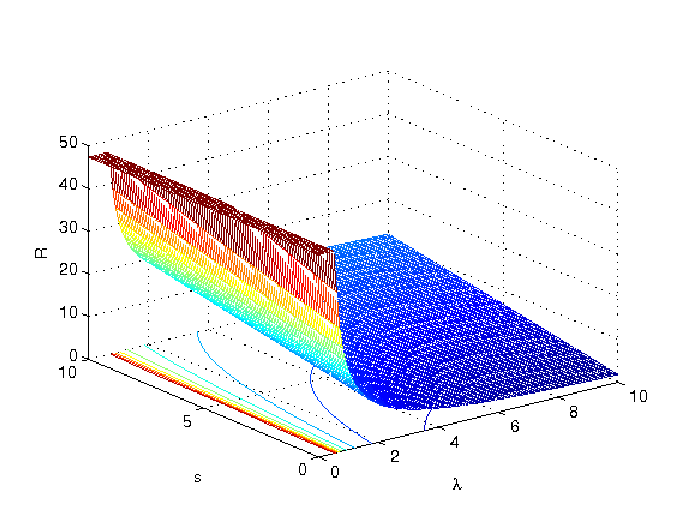
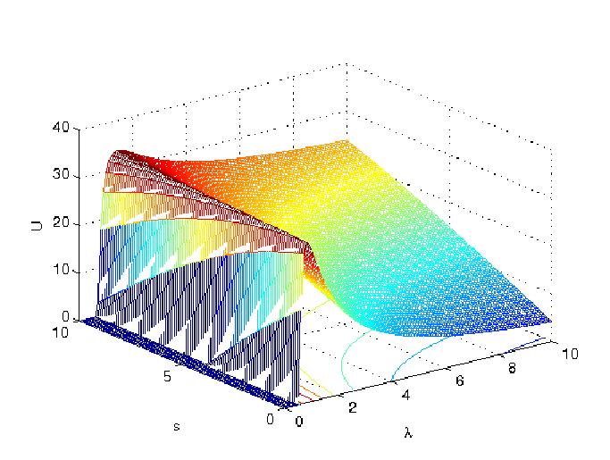
To make things clearer, consider introducing the protected areas for the healthy prey, i.e. let us give to $s$ nonzero values. In Figure 8 we plot the population levels as functions of both $\lambda$ and $s$ . Here the value of $\omega$ as said is kept at level $5$ , and independently of the fixed value of $s$ chosen, we see that the equilibrium values of the infected, center frame, as a function of $\lambda$ has a similar behavior as if no control were present, it raises up to a maximum and then decreases. As function of $s$ it is slightly decreasing. Note that the maximum of infected with no disease control for $\omega=5$ and $\lambda=2$ is about $35$ , Figure 7 center. When refuges for the healthy prey are present the number of infected remains about the same for increasing values of $s$ , Figure 8 center, probably indicating a scarce effect of this measure to contain the disease propagation.

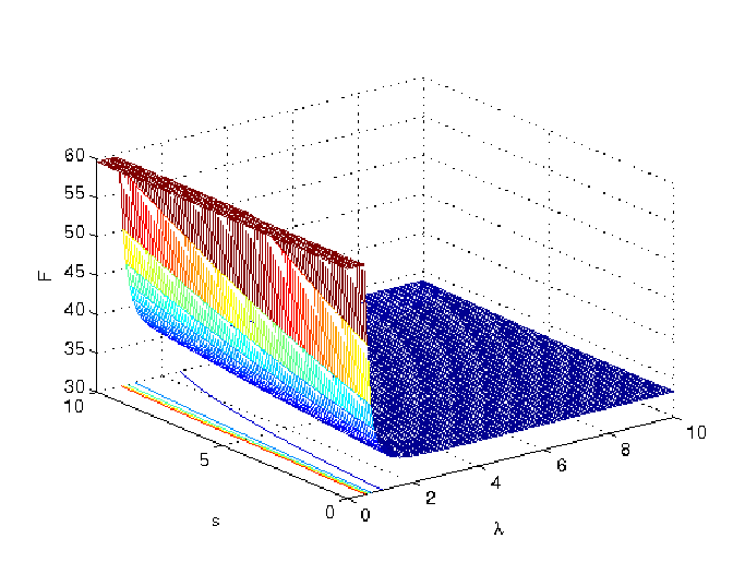
If we study the same situation as a function of the parameter $\omega$ , we have Figure 9 center, for $\lambda=0.8$ , shown under a different angle to better indicate that for large values of the control $s$ and the recovery rate $\omega$ the disease gets eradicated. Now in Figure 9 center we need to restrict the surface to the plane $\omega=5$ . The resulting function decreases with increasing $s$ , starting from a value that for $s$ close to zero is comparable to the reference one.

If we compare the healthy prey equilibrium values, for $s\approx 0$ and $\omega=5$ , Figure 8 top, the situation is similar to the case of no disease control, Figure 7 top. Supplying the healthy prey refuges, has the benefit that the equilibrium level of the latter increase, e.g. for $s=10$ and $\lambda=10$ we find $R=10$ , certainly higher than the level in Figure 7 top for $\omega=5$ and for the corresponding value of $\lambda=10$ . Similarly we find that as a function of $\omega$ the equilibrium level surface is almost always above the level $R=10$ , thus improving over the case of no control, Figure 9 top. In particular in this latter case the increase in number of healthy prey is quite dramatic.

7.7 Comparison of the four different controls

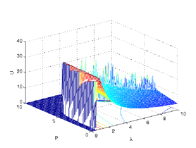
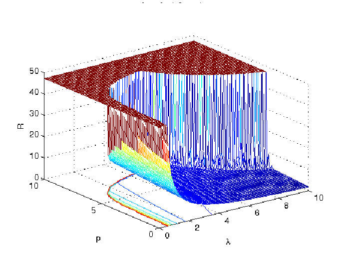
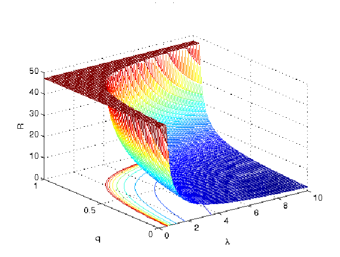
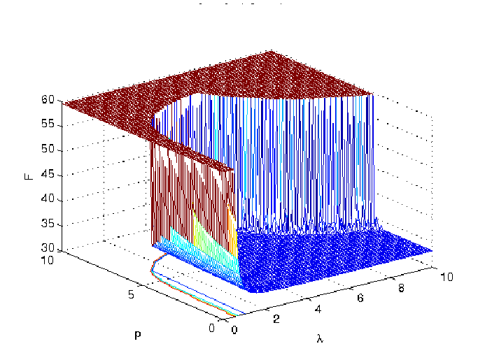
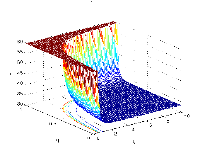
We now consider the four different controls. Plotting in the same frame the infected as function of all of them and of $\lambda$ , Figure 10, left to right and top to bottom the controls being $s$ , $p$ , $q$ and $\delta$ , we observe some differences in the infected equilibrium levels. As already discussed above, the parameter $s$ seems to lead in general to a rather higher prevalence, uniformly and independently of the contact rate $\lambda$ . A sufficiently high value of both $p$ and $q$ , for not too high values of $\lambda$ , lead to disease eradication, e.g. $\lambda=1$ and $p=7$ or $q=0.7$ . However, both seem to have drawbacks: the “inappropriate” use of $p$ or $q$ leads to a high peak in the prevalence, for $\lambda\approx 2$ and $q\approx 0.7$ . This occurs throughout the possible ranges of the controls and of the disease transmission rate, following the peaks in the two frames. The difference however is that the peak is rather steady when the control $q$ is used, while it decreases slowly in case of $p$ . So among these two controls, the refuge for the infected prey is preferable. In fact, in this case a choice of a large $p$ when $\lambda$ is also large leads to persistent oscillations, as remarked earlier, Figure 6, which correspond to the uneven portion of the surface in the upper right corner of Figure 10, frame for the control $p$ .

Culling markedly decreases the peak of the prevalence when $\lambda=0.8$ , but it gives a much smaller range for which the disease is eradicated compared to the use of $q$ and $p$ . The “zero level” surface has a larger area indeed in the frames for the reduced contacts and the refuges for infected prey controls than what we find in the frame for culling. For large values of the transmission rate and low levels of the controls $p$ , $q$ and $\delta$ the number of infected at equilibrium settles to about the same value $U=10$ . For larger implementations of these controls however, there is a marked difference. For $q$ the prevalence shoots up and only for extreme values of the control it goes down and eventually disappears. When using culling, the infected equilibrium levels do not change much even if high rates of abatement are employed. For the refuges for infected prey strategy, prevalence remains about the same, then there is a regime of oscillatory behavior, and finally for larger values of the control the disease is eradicated.

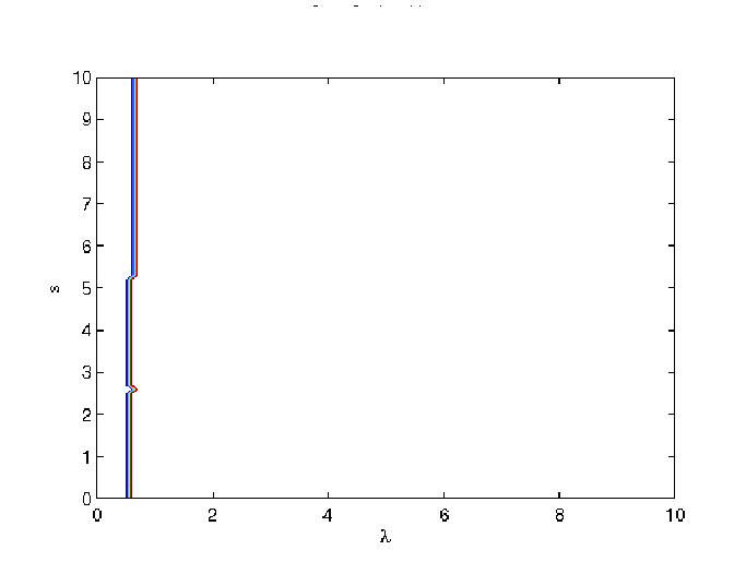
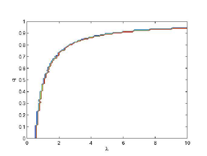
To better study the limit cycles, we plot in Figure 11 the parameter space of the controls used versus the disease transmission rate. The curves in each plot separate the region in which the disease is eradicated, the one having as border the vertical axis, from the region where the disease is endemic, the one bordering the horizontal axis. The region of the limit cycles appears only when the $p$ control is used, at the interface of the two regimes, for large values of the contact rate $\lambda$ . The largest area for the disease-free equilibrium is therefore observed in case control is exercised through the parameter $p$ .

In Figure 12 we also compare the loci of the equilibria in the various controls versus the disease recovery rate parameter space. Here the region containing the origin represents always the endemic equilibrium. The $s$ control exhibits the smallest disease-free equilibrium region, the very small triangle in the top right corner. Similarly to it behaves culling. The reduced contacts and the refuge for infected prey controls have much larger regions where the disease is eradicated, with the largest region apparently being provided by the former policy, recalling that $q$ is a fraction and cannot exceed 1.

Comparing the healthy prey and predators levels, Figures 13 and 14, similar conclusions can be drawn. Culling and refuge for the healthy prey seem to behave similarly to each other, certainly less effectively than the other two policies. Among these two, as far as the healthy prey are concerned, it seems to be preferable not to use culling, since for large transmission rate $\lambda\approx 10$ , for high values of the control $s$ , they have a value around 10, while they attain much smaller values independently of the culling rate used. The predators levels are instead about the same for both policies also for large $\lambda$ . The policies of refuges for the infected prey and of reducing the contact rate instead, when heavily implemented, i.e. for large values of the parameters $p$ and $q$ , boost both healthy prey and predators populations levels, especially in presence of high transmission rates, see the left top corners of the corresponding figures. A clear advantage is obtained by providing refuges for the infected prey, where they are less able to transmit the disease, see the top right frames in both Figures 13 and 14.

7.8 Final considerations

In summary it seems that no strategy is the best alone. A clear exception are the safety refuges for healthy prey, in that they do not seem to be effective in controlling the disease levels and therefore should not be used. Selective culling on infected prey has adverse effects on healthy prey and predators, but it is preferable to control through reduced contacts in terms of smaller disease prevalence. In presence of a high transmission rate the best policy is to use refuges for the infected individuals, taking into account however that an insufficient use of this control may trigger persistent oscillations in the system.

Thus in this type of predator-prey ecoepidemic system with disease just in the prey, for an endemic disease, the ecosystem with a place where some of the healthy individuals can be segregated from coming in contact with disease carriers would exhibit the worst features to preserve the epidemics to spread. Probably the most indicated strategies are providing areas for the infected prey where they cannot come in contact with the healthy ones, Reducing the contact rate and culling seem instead to have mixed effects. This result could possibly give some hints to field ecologists as how to fight diseases in wild populations, in case some artificial refuges for the diseased individuals, unreachable by the healthy animals, can be provided in specific real-life situations.

Acknowledgements.

EV is indebted to Prof. Cristobal Vargas for a useful discussion upon this matter, leading to the analysis of the model with culling. This research was partially supported by the project “Metodi numerici in teoria delle popolazioni” of the Dipartimento di Matematica “Giuseppe Peano”.

References

(1) J. B. Collings, Bifurcations and stability analysis of a temperature-dependent mite predator-prey interaction model incorporating a prey refuge, Bulletin of Mathematical Biology 57 (1995) 63-76.
(2) E. González-Olivares, R. Ramos-Jiliberto, Dynamic consequences of prey refuges in a simple model system: more prey, fewer predators and enhanced stability, Ecological Modelling 166 (2003) 135-146.
(3) E. González-Olivares, R. Ramos-Jiliberto, Comments to the effect of prey refuge in a simple predator-prey model, Ecological Modelling 232 (2012) 158-160.
(4) Kuno E. (1987) Principles of predator-prey interactions in theoretical, experimental, and natural population systems, Advances in Ecological Researches 16, 249-337.
(5) H. Malchow, S. Petrovskii, E. Venturino, Spatiotemporal patterns in Ecology and Epidemiology, CRC, Boca Raton, 2008.
(6) May R.A. (1973) Stability and complexity in model ecosystems, Monographs in population biology, 6, New Jersey, Princeton University Press
(7) May R.A. (1976) Simple mathematical models with very complicated structure, Nature 261, 459-467
(8) Maynard Smith J. (1974) Models in ecology, Cambridge University Press, Cambridge.
(9) G. D. Ruxton, Short term refuge use and stability of predator-prey models, Theoretical Population Biology 47 (1995) 1-17.
(10) E. Venturino, Epidemics in predator-prey models: disease among the prey, in O. Arino, D. Axelrod, M. Kimmel, M. Langlais: Mathematical Population Dynamics: Analysis of Heterogeneity, Vol. one: Theory of Epidemics, Wuertz Publishing Ltd, Winnipeg, Canada, (1995) 381-393.