The unstable set of a periodic orbit for delayed positive feedback

Abstract.

In the paper [Large-amplitude periodic solutions for differential equations with delayed monotone positive feedback, JDDE 23 (2011), no. 4, 727–790], we have constructed large-amplitude periodic orbits for an equation with delayed monotone positive feedback. We have shown that the unstable sets of the large-amplitude periodic orbits constitute the global attractor besides spindle-like structures. In this paper we focus on a large-amplitude periodic orbit $\mathcal{O}_{p}$ with two Floquet multipliers outside the unit circle, and we intend to characterize the geometric structure of its unstable set $\mathcal{W}^{u}\left(\mathcal{O}_{p}\right)$ . We prove that $\mathcal{W}^{u}\left(\mathcal{O}_{p}\right)$ is a three-dimensional $C^{1}$ -submanifold of the phase space and admits a smooth global graph representation. Within $\mathcal{W}^{u}\left(\mathcal{O}_{p}\right)$ , there exist heteroclinic connections from $\mathcal{O}_{p}$ to three different periodic orbits. These connecting sets are two-dimensional $C^{1}$ -submanifolds of $\mathcal{W}^{u}\left(\mathcal{O}_{p}\right)$ and homeomorphic to the two-dimensional open annulus. They form $C^{1}$ -smooth separatrices in the sense that they divide the points of $\mathcal{W}^{u}\left(\mathcal{O}_{p}\right)$ into three subsets according to their $\omega$ -limit sets.

Tibor Krisztin¹¹ 1 e-mail: krisztin@math.u-szeged.hu, Gabriella Vas²² 2 e-mail: vasg@math.u-szeged.hu

MTA-SZTE Analysis and Stochastic Research Group, Bolyai Institute, University of Szeged, Hungary

Key words: Delay differential equation, Positive feedback, Periodic orbit, Unstable set, Floquet theory, Poincaré map, Invariant manifold, Lyapunov functional, Transversality

Suggested running head: The unstable set of a periodic orbit

AMS Subject Classification: 34K13, 34K19, 37C70, 37D05, 37L25, 37L45

1. Introduction

Consider the delay differential equation

(1.1)

\dot{x}\left(t\right)=-\mu x\left(t\right)+f\left(x\left(t-1\right)\right),

where $\mu$ is a positive constant and $f:\mathbb{R}\rightarrow\mathbb{R}$ is a smooth monotone nonlinearity.

The natural phase space for Eq. (1.1) is $C=C\left(\left[-1,0\right],\mathbb{R}\right)$ equipped with the supremum norm. For any $\varphi\in C$ , there is a unique solution $x^{\varphi}:\left[-1,\infty\right)\rightarrow\mathbb{R}$ of (1.1). For each $t\geq 0$ , $x_{t}^{\varphi}\in C$ is defined by $x_{t}^{\varphi}\left(s\right)=x^{\varphi}\left(t+s\right)$ , $-1\leq s\leq 0$ . Then the map

\Phi:\left[-1,\infty\right)\times C\ni\left(t,\varphi\right)\mapsto x_{t}^{\varphi}\in C

is a continuous semiflow.

In [8], the authors of this paper have studied Eq. (1.1) under the subsequent hypothesis:

(H1)

$\mu>0$ , $f\in C^{1}\left(\mathbb{R},\mathbb{R}\right)$ with $f^{\prime}\left(\xi\right)>0$ for all $\xi\in\mathbb{R}$ , and

$\xi_{-2}<\xi_{-1}<\xi_{0}=0<\xi_{1}<\xi_{2}$

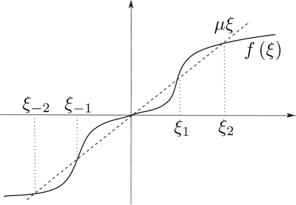
are five consecutive zeros of $\mathbb{R}\ni\xi\mapsto-\mu\xi+f\left(\xi\right)\in\mathbb{R}$ with $f^{\prime}\left(\xi_{j}\right)<\mu<f^{\prime}\left(\xi_{k}\right)$ for $j\in\left\{-2,0,2\right\}$ and $k\in\left\{-1,1\right\}$ (see Fig. 1).

Refer to caption — Figure 1. A feedback function satisfying condition (H1).

Under hypothesis (H1), $\hat{\xi}_{j}\in C$ , defined by $\hat{\xi}_{j}\left(s\right)=\xi_{j}$ , $-1\leq s\leq 0$ , is an equilibrium point of $\Phi$ for all $j\in\left\{-2,-1,0,1,2\right\}$ , furthermore $\hat{\xi}_{-2},$ $\hat{\xi}_{0}$ and $\hat{\xi}_{2}$ are stable, and $\hat{\xi}_{-1}$ and $\hat{\xi}_{1}$ are unstable. By the monotone property of $f$ , the subsets

C_{-2,2}=\left\{\varphi\in C:\,\xi_{-2}\leq\varphi\left(s\right)\leq\xi_{2}\mbox{ for all }s\in\left[-1,0\right]\right\},

C_{-2,0}=\left\{\varphi\in C:\,\xi_{-2}\leq\varphi\left(s\right)\leq 0\mbox{ for all }s\in\left[-1,0\right]\right\},

C_{0,2}=\left\{\varphi\in C:\,0\leq\varphi\left(s\right)\leq\xi_{2}\mbox{ for all }s\in\left[-1,0\right]\right\}

of the phase space $C$ are positively invariant under the semiflow $\Phi$ (see Proposition 2.4 in Section 2).

Let $\mathcal{A}$ , $\mathcal{A}_{-2,0}$ and $\mathcal{A}_{0,2}$ denote the global attractors of the restrictions $\Phi|_{\left[0,\infty\right)\times C_{-2,2}}$ , $\Phi|_{\left[0,\infty\right)\times C_{-2,0}}$ and $\Phi|_{\left[0,\infty\right)\times C_{0,2}}$ , respectively. If (H1) holds and $\xi_{-2},\xi_{-1},0,\xi_{1},\xi_{2}$ are the only zeros of $-\mu\xi+f\left(\xi\right)$ , then $\mathcal{A}$ is the global attractor of $\Phi$ . The structures of $\mathcal{A}_{-2,0}$ and $\mathcal{A}_{0,2}$ are (at least partially) well understood, see e.g. [5, 6, 7, 9, 10, 11]. $\mathcal{A}_{-2,0}$ and $\mathcal{A}_{0,2}$ admit Morse decompositions [18]. Further technical conditions regarding $f$ ensure that $\mathcal{A}_{-2,0}$ and $\mathcal{A}_{0,2}$ have spindle-like structures [5, 9, 10, 11]: $\mathcal{A}_{0,2}$ is the closure of the unstable set of $\hat{\xi}_{1}$ containing the equilibrium points $\hat{\xi}_{0}$ , $\hat{\xi}_{1}$ , $\hat{\xi}_{2}$ , periodic orbits in $C_{0,2}$ and heteroclinic orbits among them. In other cases $\mathcal{A}_{0,2}$ is larger than the the closure of the unstable set of $\hat{\xi}_{1}$ . The structure of $\mathcal{A}_{-2,0}$ is similar. See Fig. 2 for a simple situation.

The monograph [10] of Krisztin, Walther and Wu has addressed the question whether the equality $\mathcal{A}=\mathcal{A}_{-2,0}\cup\mathcal{A}_{0,2}$ holds under hypothesis (H1). The authors of this paper have constructed an example in [8] so that (H1) holds, and Eq. (1.1) admits periodic orbits in $\mathcal{A}\setminus\left(\mathcal{A}_{-2,0}\cup\mathcal{A}_{0,2}\right)$ , that is, besides the spindle-like structures. The periodic solutions defining these periodic orbits oscillate slowly around $0$ and have large amplitudes in the following sense.

A periodic solution $r:\mathbb{R}\rightarrow\mathbb{R}$ of Eq. (1.1) is called a large amplitude periodic solution if $r(\mathbb{R})\supset(\xi_{-1},\xi_{1})$ . A solution $r:\mathbb{R}\rightarrow\mathbb{R}$ is slowly oscillatory if for each $t$ , the restriction $r|_{[t-1,t]}$ has one or two sign changes. Note that here slow oscillation is different from the usual one used for equations with negative feedback condition [2, 21]. A large-amplitude slowly oscillatory periodic solution $r:\mathbb{R}\rightarrow\mathbb{R}$ is abbreviated as an LSOP solution. We say that an LSOP solution $r:\mathbb{R}\rightarrow\mathbb{R}$ is normalized if $r(-1)=0$ , and for some $\eta>0$ , $r(s)>0$ for all $s\in(-1,-1+\eta)$ .

The first main result of [8] is as follows.

Theorem A.

There exist $\mu$ and $f$ satisfying (H1) such that Eq. (1.1) has exactly two normalized LSOP solutions $p:\mathbb{R}\rightarrow\mathbb{R}$ and $q:\mathbb{R}\rightarrow\mathbb{R}$ . For the ranges of $p$ and $q$ , $(\xi_{-1},\xi_{1})\subset p(\mathbb{R})\subset q(\mathbb{R})\subset\left(\xi_{-2},\xi_{2}\right)$ holds. The corresponding periodic orbits

\mathcal{O}_{p}=\left\{p_{t}:\,t\in\mathbb{R}\right\}\ \mathit{and}\ \mathcal{O}_{q}=\left\{q_{t}:\,t\in\mathbb{R}\right\}

are hyperbolic and unstable. $\mathcal{O}_{p}$ admits two different Floquet multipliers outside the unit circle, which are real and simple. $\mathcal{O}_{q}$ has one real simple Floquet multiplier outside the unit circle.

Note that although Theorem 1.1 in [8] does not mention that the Floquet multipliers found outside the unit circle are simple and real, these properties are verified in Section 4 of the same paper.

In the proof of the theorem, $\mu=1$ and $f$ is close to the step function

f^{K,0}\left(x\right)=\begin{cases}-K&\mbox{if }x<-1,\\ 0&\mbox{if }\left|x\right|\leq 1,\\ K&\mbox{if }x>1,\end{cases}

where $K>0$ is chosen large enough.

In their paper [3], Fiedler, Rocha and Wolfrum considered a special class of one-dimensional parabolic partial differential equations and obtained a catalogue listing the possible structures of the global attractor. In particular, the result of Theorem A motivated Fiedler, Rocha and Wolfrum to find an analogous configuration for their equation. It is an interesting question whether all the structures found by them have counterparts in the theory of Eq. (1.1).

Let $\mathcal{W}^{u}\left(\mathcal{O}_{p}\right)$ and $\mathcal{W}^{u}\left(\mathcal{O}_{q}\right)$ denote the unstable sets of $\mathcal{O}_{p}$ and $\mathcal{O}_{q}$ , respectively.

A solution $r:\mathbb{R}\rightarrow\mathbb{R}$ is called slowly oscillatory around $\xi_{k}$ , $k\in\left\{-1,1\right\}$ , if $\mathbb{R}\ni t\mapsto r(t)-\xi_{k}\in\mathbb{R}$ admits one or two sign changes on each interval of length $1$ . As it is described by Proposition 2.7 in [8], $f$ and $\mu$ in Theorem A are set so that there exist at least one periodic solution oscillating slowly around $\xi_{1}$ with range in $(0,\xi_{2})$ , furthermore there is a solution $x^{1}:\mathbb{R}\rightarrow\mathbb{R}$ among such periodic solutions that has maximal range $x^{1}(\mathbb{R})$ in the sense that $x^{1}(\mathbb{R})\supset x(\mathbb{R})$ for all periodic solutions $x$ oscillating slowly around $\xi_{1}$ with range in $(0,\xi_{2})$ . Similarly, there exists a maximal periodic solution $x^{-1}$ oscillating slowly around $\xi_{-1}$ with range in $(\xi_{-2},0)$ . Set

\mathcal{O}_{1}=\left\{x_{t}^{1}:t\in\mathbb{R}\right\}\mbox{ and }\mathcal{O}_{-1}=\left\{x_{t}^{-1}:t\in\mathbb{R}\right\}.

Let $\omega\left(\varphi\right)$ denote the $\omega$ -limit set of any $\varphi\in C$ . Introduce the connecting sets

\displaystyle C_{j}^{p}=

\displaystyle\left\{\varphi\in\mathcal{W}^{u}\left(\mathcal{O}_{p}\right):\,\omega\left(\varphi\right)=\hat{\xi}_{j}\right\},\qquad j\in\left\{-2,0,2\right\},

\displaystyle C_{k}^{p}=

\displaystyle\left\{\varphi\in\mathcal{W}^{u}\left(\mathcal{O}_{p}\right):\,\omega\left(\varphi\right)=\mathcal{O}_{k}\right\},\qquad k\in\left\{-1,1\right\},

and

\displaystyle C_{q}^{p}=

\displaystyle\left\{\varphi\in\mathcal{W}^{u}\left(\mathcal{O}_{p}\right):\,\omega\left(\varphi\right)=\mathcal{O}_{q}\right\}.

Sets $C_{j}^{q}$ , $j\in\left\{-2,2\right\}$ , are defined analogously.

The next theorem has also been given in [8] and describes the dynamics in $\mathcal{A}\setminus(\mathcal{A}_{-2,0}\cup\mathcal{A}_{0,2})$ .

Theorem B.

One may set $\mu$ and $f$ satisfying (H1) such that the statement of Theorem A holds, and for the global attractor $\mathcal{A}$ we have the equality

\mathcal{A}=\mathcal{A}_{-2,0}\cup\mathcal{A}_{0,2}\cup\mathcal{W}^{u}\left(\mathcal{O}_{p}\right)\cup\mathcal{W}^{u}\left(\mathcal{O}_{q}\right).

Moreover, the dynamics on $\mathcal{W}^{u}\left(\mathcal{O}_{p}\right)$ and $\mathcal{W}^{u}\left(\mathcal{O}_{q}\right)$ is as follows. The connecting sets $C_{j}^{p}$ , $C_{q}^{p}$ , $C_{k}^{p}$ , $j\in\left\{-2,0,2\right\}$ , $k\in\left\{-1,1\right\}$ , are nonempty, and

\mathcal{W}^{u}\left(\mathcal{O}_{p}\right)=\mathcal{O}_{p}\cup C_{-2}^{p}\cup C_{-1}^{p}\cup C_{0}^{p}\cup C_{1}^{p}\cup C_{2}^{p}\cup C_{q}^{p}.

The connecting sets $C_{-2}^{q}$ and $C_{2}^{q}$ are nonempty, and

\mathcal{W}^{u}\left(\mathcal{O}_{q}\right)=\mathcal{O}_{q}\cup C_{-2}^{q}\cup C_{2}^{q}.

The system of heteroclinic connections is represented in Fig. 3.

Figure 3. Connecting orbits: the dashed arrows represent heteroclinic connections in

\mathcal{A}_{-2,0}

and in

\mathcal{A}_{0,2}

, while the solid ones represent connecting orbits given by Theorem B.

Hereinafter we fix $\mu=1$ and set $f$ in Eq. (1.1) so that Theorems A and B hold. The purpose of this paper is to characterize the geometrical properties of $\mathcal{W}^{u}\left(\mathcal{O}_{p}\right)$ and the connecting sets within $\mathcal{W}^{u}\left(\mathcal{O}_{p}\right)$ .

We say that a subset $W$ of $C$ admits global graph representation, if there exists a splitting $C=G\oplus E$ with closed subspaces $G$ and $E$ of $C$ , a subset $U$ of $G$ and a map $w:U\rightarrow E$ such that

W=\left\{\chi+w\left(\chi\right):\,\chi\in U\right\}.

$W$ is said to have a smooth global graph representation if in the above definition $U$ is open in $G$ and $w$ is $C^{1}$ -smooth on $U$ . Note that in this case $W$ is a $C^{1}$ -submanifold of $C$ in the usual sense with dimension $\dim G$ , see e.g. the definition of Lang in [12]. $W$ is said to admit a smooth global graph representation with boundary if $G$ is $n$ dimensional with some integer $n\geq 1$ , $U$ is the closure of an open set $U^{0}$ , $w$ is $C^{1}$ -smooth on $U^{0}$ , the boundary $\mbox{bd}U$ of $U$ in $G$ is an $(n-1)$ -dimensional $C^{1}$ -submanifold of $G$ , and all points of $\mbox{bd}U$ have an open neighborhood in $G$ on which $w$ can be extended to a $C^{1}$ -smooth function. In this case $W$ is an $n$ -dimensional $C^{1}$ -submanifold of $C$ with boundary in the usual sense [12].

The first result of this paper is the following.

Theorem 1.1.

$\mathcal{W}^{u}\left(\mathcal{O}_{p}\right)$ , $C_{-2}^{p},\,C_{0}^{p}$ and $C_{2}^{p}$ are three-dimensional $C^{1}$ -submanifolds of $C$ admitting smooth global graph representations.

The next objects of our study are the connecting sets $C_{q}^{p}$ , $C_{-1}^{p}$ , $C_{1}^{p}$ containing the heteroclinic orbits from $\mathcal{O}_{p}$ to $\mathcal{O}_{q}$ , $\mathcal{O}_{-1}$ , $\mathcal{O}_{1}$ , respectively. We actually get a detailed picture of the structure of $\mathcal{W}^{u}\left(\mathcal{O}_{p}\right)$ by characterizing the unions

S_{-1}=C_{-1}^{p}\cup\mathcal{O}_{p}\cup C_{q}^{p}\qquad\mbox{and}\qquad S_{1}=C_{1}^{p}\cup\mathcal{O}_{p}\cup C_{q}^{p}.

A solution $x:\mathbb{R}\rightarrow\mathbb{R}$ is said to oscillate around $\xi_{i}$ , $i\in\left\{-2,-1,0,1,2\right\}$ , if the set $x^{-1}\left(\xi_{i}\right)\subset\mathbb{R}$ is not bounded from above. It is a direct consequence of Theorem B that for $k\in\left\{-1,1\right\}$ ,

(1.2)

S_{k}=\left\{\varphi\in\mathcal{W}^{u}\left(\mathcal{O}_{p}\right):\,x^{\varphi}\mbox{ oscillates around }\xi_{k}\right\}.

We say that a subset $W$ of $\mathcal{W}^{u}\left(\mathcal{O}_{p}\right)$ is above $S_{k}$ , $k\in\left\{-1,1\right\}$ , if to each $\varphi\in W$ there corresponds an element $\psi$ of $S_{k}$ with $\psi\ll\varphi$ (that is, $\psi\left(s\right)<\varphi\left(s\right)$ for all $s\in\left[-1,0\right]$ ). Similarly, a subset $W$ of $\mathcal{W}^{u}\left(\mathcal{O}_{p}\right)$ is below $S_{k}$ , $k\in\left\{-1,1\right\}$ , if for all $\varphi\in W$ there exists $\psi\in S_{k}$ with $\varphi\ll\psi$ . $W$ is between $S_{-1}$ and $S_{1}$ if it is below $S_{1}$ and above $S_{-1}$ .

Our main result offers geometrical and topological descriptions of $C_{q}^{p}$ , $C_{-1}^{p}$ , $C_{1}^{p}$ , $S_{-1}$ and $S_{1}$ , and their closures in $C$ . It shows that $S_{-1}$ and $S_{1}$ separate the points of $\mathcal{W}^{u}\left(\mathcal{O}_{p}\right)$ into three groups according to their $\omega$ -limit sets. Thereby, $S_{-1}$ and $S_{1}$ play a key role in the dynamics of the equation.

Theorem 1.2.

(i) The sets $C_{q}^{p}$ , $C_{-1}^{p}$ , $C_{1}^{p}$ , $S_{-1}$ and $S_{1}$ are two-dimensional $C^{1}$ -submanifolds of $\mathcal{W}^{u}\left(\mathcal{O}_{p}\right)$ with smooth global graph representations. They are homeomorphic to the open annulus

A^{\left(1,2\right)}=\left\{u\in\mathbb{R}^{2}:\,1<\left|u\right|<2\right\}.

(ii) The equalities

\overline{C_{q}^{p}}=\mathcal{O}_{p}\cup C_{q}^{p}\cup\mathcal{O}_{q},\qquad\overline{C_{k}^{p}}=\mathcal{O}_{p}\cup C_{k}^{p}\cup\mathcal{O}_{k}

and

\overline{S_{k}}=\mathcal{O}_{k}\cup S_{k}\cup\mathcal{O}_{q}=\mathcal{O}_{k}\cup C_{k}^{p}\cup\mathcal{O}_{p}\cup C_{q}^{p}\cup\mathcal{O}_{q}

hold for both $k\in\left\{-1,1\right\}$ . The sets $\overline{C_{q}^{p}}$ , $\overline{C_{-1}^{p}}$ , $\overline{C_{1}^{p}}$ , $\overline{S_{-1}}$ and $\overline{S_{1}}$ admit smooth global graph representations with boundary, and thereby they are two-dimensional $C^{1}$ -submanifolds of $C$ with boundary. In addition, they are homeomorphic to the closed annulus

A^{\left[1,2\right]}=\left\{u\in\mathbb{R}^{2}:\,1\leq\left|u\right|\leq 2\right\}.

(iii) $S_{{}_{-1}}$ and $S_{1}$ are separatrices in the sense that $C_{2}^{p}$ is above $S_{1}$ , $C_{0}^{p}$ is between $S_{-1}$ and $S_{1}$ , furthermore $C_{-2}^{p}$ is below $S_{-1}$ .

Fig. 4 visualizes the structure of the closure $\overline{\mathcal{W}^{u}\left(\mathcal{O}_{p}\right)}$ of $\mathcal{W}^{u}\left(\mathcal{O}_{p}\right)$ in $C$ . To get an overview of the above results regarding $\mathcal{W}^{u}\left(\mathcal{O}_{p}\right)$ , see the inner part of Fig. 4, drawn in black. We emphasize a particular consequence of Theorem 1.2: the tangent spaces of $S_{-1}$ and $S_{1}$ coincide along $\mathcal{O}_{p}$ , see Fig. 5.

Let $\mathcal{W}^{u}\left(\mathcal{O}_{1}\right)$ and $\mathcal{W}^{u}\left(\mathcal{O}_{-1}\right)$ denote the unstable sets of $\mathcal{O}_{1}$ and $\mathcal{O}_{-1}$ , respectively, defined as the forward extension of a one-dimensional local unstable manifold of a return map (corresponding to the only Floquet multiplier outside the unit circle which is real and simple), see (3.5). We expect $\mathcal{W}^{u}\left(\mathcal{O}_{q}\right)$ , $\mathcal{W}^{u}\left(\mathcal{O}_{-1}\right)$ and $\mathcal{W}^{u}\left(\mathcal{O}_{1}\right)$ to be two-dimensional $C^{1}$ -submanifolds of $C$ . We conjecture that for the closure $\overline{\mathcal{W}^{u}\left(\mathcal{O}_{p}\right)}$ of $\mathcal{W}^{u}\left(\mathcal{O}_{p}\right)$ in $C$ , the equality

\overline{\mathcal{W}^{u}\left(\mathcal{O}_{p}\right)}=\mathcal{W}^{u}\left(\mathcal{O}_{p}\right)\cup\mathcal{W}^{u}\left(\mathcal{O}_{q}\right)\cup\mathcal{W}^{u}\left(\mathcal{O}_{1}\right)\cup\mathcal{W}^{u}\left(\mathcal{O}_{-1}\right)\cup\left\{\hat{\xi}_{-2},\hat{0},\hat{\xi}_{2}\right\}

holds, as it represented in Fig. 4. Moreover, all points of $\mathcal{W}^{u}\left(\mathcal{O}_{q}\right)\cup\mathcal{W}^{u}\left(\mathcal{O}_{1}\right)\cup\mathcal{W}^{u}\left(\mathcal{O}_{-1}\right)$ have an open neighborhood on which the $C^{1}$ -map in the graph representation of $\mathcal{W}^{u}\left(\mathcal{O}_{p}\right)$ can be smoothly extended.

It also remains an open question whether $\mathcal{A}\setminus(\mathcal{A}_{-2,0}\cup\mathcal{A}_{0,2})$ is homeomorphic to the three-dimensional body

\mathcal{B}_{3}\left(\left(0,0,0\right),2\right)\backslash\left\{\mathcal{B}_{3}\left(\left(0,0,1\right),1\right)\cup\mathcal{B}_{3}\left(\left(0,0,-1\right),1\right)\right\}\subset\mathbb{R}^{3},

where $\mathcal{B}_{3}\left(\left(a_{1},a_{2},a_{3}\right),r\right)$ denotes the three-dimensional closed ball with center $\left(a_{1},a_{2},a_{3}\right)$ and radius $r$ .

The proofs of Theorems 1.1–1.2 apply general results on delay differential equations, the Floquet theory (Appendix VII of [10], [14]), results on local invariant manifolds for maps in Banach spaces (Appendices I-II of [10]), correspondences between different return maps (Appendices I and V of [10]), a result from transversality theory [1] and also a discrete Lyapunov functional of Mallet-Paret and Sell counting the sign changes of the elements of $C$ (Appendix VI of [10], [16]).

This paper is organized as follows. Section 2 offers a general overview of the theoretical background and introduces the discrete Lyapunov functional. As the Floquet theory and certain results on local invariant manifolds of return maps play essential role in this work, Section 3 is devoted to the discussion of these concepts. Sections 4 and 5 contain the proofs of Theorems 1.1 and 1.2, respectively.

The proof of Theorem 1.1 in Section 4 takes advantage of the fact that the unstable set of a hyperbolic periodic orbit is the forward continuation of a local unstable manifold of a Poincaré map by the semiflow. In consequence, by using the smoothness of the local unstable manifold and the injectivity of the derivative of the solution operator, we prove that all points $\varphi$ of $\mathcal{W}^{u}\left(\mathcal{O}_{p}\right)$ belong to a subset $W_{\varphi}$ of $\mathcal{W}^{u}\left(\mathcal{O}_{p}\right)$ that is a three-dimensional $C^{1}$ -submanifold of $C$ . This means that $\mathcal{W}^{u}\left(\mathcal{O}_{p}\right)$ is an immersed submanifold of $C$ . In general, an immersed submanifold is not necessarily an embedded submanifold of the phase space. In order to prove that $\mathcal{W}^{u}\left(\mathcal{O}_{p}\right)$ is embedded in $C$ , we have to show that for any $\varphi$ in $\mathcal{W}^{u}\left(\mathcal{O}_{p}\right)$ , there is no sequence in $\mathcal{W}^{u}\left(\mathcal{O}_{p}\right)\backslash W_{\varphi}$ converging to $\varphi$ . We define a projection $\pi_{3}$ from $C$ into $\mathbb{R}^{3}$ . Using well-known properties of the discrete Lyapunov functional, we show that $\pi_{3}$ is injective on $\mathcal{W}^{u}\left(\mathcal{O}_{p}\right)$ and on the tangent spaces of $W_{\varphi}$ . This implies that $\pi_{3}W_{\varphi}$ is open in $\mathbb{R}^{3}$ . If a sequence $\left(\varphi^{n}\right)_{n=0}^{\infty}$ in $\mathcal{W}^{u}\left(\mathcal{O}_{p}\right)\backslash W_{\varphi}$ converges to $\varphi$ as $n\rightarrow\infty$ , then $\pi_{3}\varphi^{n}\rightarrow\pi_{3}\varphi$ as $n\rightarrow\infty$ , and $\pi_{3}\varphi^{n}\in\pi_{3}W_{\varphi}$ for all $n$ large enough. The injectivity of $\pi_{3}$ on $\mathcal{W}^{u}\left(\mathcal{O}_{p}\right)$ then implies that $\varphi^{n}\in W_{\varphi}$ , which is a contradiction. So $\mathcal{W}^{u}\left(\mathcal{O}_{p}\right)$ is a three-dimensional embedded $C^{1}$ -submanifold of the phase space. The description of $\mathcal{W}^{u}\left(\mathcal{O}_{p}\right)$ is rounded up by giving a graph representation for $\mathcal{W}^{u}\left(\mathcal{O}_{p}\right)$ in order to present the simplicity of it structure. The smoothness of the sets $C_{-2}^{p},\,C_{0}^{p}$ and $C_{2}^{p}$ then follows at once because they are open subsets of $\mathcal{W}^{u}\left(\mathcal{O}_{p}\right)$ . We also obtain as an important consequence that the semiflow defined by the solution operator extends to a $C^{1}$ -flow on $\mathcal{W}^{u}\left(\mathcal{O}_{p}\right)$ with injective derivatives.

The proof of Theorem 1.2 in Section 5 is built from several steps, and it is organized into five subsections.

In Subsection 5.1 we list preliminary results regarding the closure $\overline{S_{k}}$ of $S_{k}$ in $C$ , $k\in\left\{-1,1\right\}$ . We introduce in particular a projection $\pi_{2}$ from $C$ into $\mathbb{R}^{2}$ , and – using the special properties of the discrete Lyapunov functional – we show that $\pi_{2}$ is injective on $\overline{S_{k}}$ . The injectivity of $\pi_{2}|_{\overline{S_{k}}}$ is already sufficient to give a two-dimensional graph representation for any subset $W$ of $\overline{S_{k}}$ (without smoothness properties): there is a linear isomorphism $J_{2}:\mathbb{R}^{2}\rightarrow C$ such that $P_{2}=J_{2}\circ\pi_{2}:C\rightarrow C$ is a projection onto a two-dimensional subspace $G_{2}$ of $C$ , and there exists a map $w_{k}$ defined on the image set $P_{2}\overline{S_{k}}$ with range in $P_{2}^{-1}\left(0\right)$ such that for any subset $W\subseteq S_{k}$ ,

W=\left\{\chi+w_{k}\left(\chi\right):\,\chi\in P_{2}W\right\}.

The smoothness of $w_{k}$ and the properties of its domain $P_{2}\overline{S_{k}}\subset G_{2}$ are investigated later. Subsection 5.1 is closed with showing that $\pi_{2}|_{\overline{S_{k}}}$ is a homeomorphism onto its image, furthermore $\pi_{2}$ is injective on the tangent spaces of $\overline{S_{k}}$ .

It is clear that $\left(\mathcal{O}_{k}\cup S_{k}\cup\mathcal{O}_{q}\right)\subset\overline{S_{k}}$ for both $k\in\left\{-1,1\right\}$ . The converse inclusion is proved in Subsection 5.2 based on the previously obtained result that $\overline{S_{k}}$ is mapped injectively into $\mathbb{R}^{2}$ . Then it follows easily that $\overline{C_{k}^{p}}$ , $k\in\left\{-1,1\right\},$ and $\overline{C_{q}^{p}}$ are not larger than the unions $\mathcal{O}_{p}\cup C_{k}^{p}\cup\mathcal{O}_{k}$ and $\mathcal{O}_{p}\cup C_{q}^{p}\cup\mathcal{O}_{q}$ , respectively.

It is a more challenging task to show that $C_{q}^{p}$ and $C_{k}^{p}$ , $k\in\left\{-1,1\right\},$ are $C^{1}$ -submanifolds of $\mathcal{W}^{u}\left(\mathcal{O}_{p}\right)$ (as stated by Theorem 1.2.(i)). The proof of this assertion is contained in Subsection 5.3. It is partly based on transversality [1]; we verify that $\mathcal{W}^{u}\left(\mathcal{O}_{p}\right)$ intersects transversally a local center-stable manifold of a Poincaré return map at a point of $\mathcal{O}_{k}$ and a local stable manifold of a Poincaré return map at a point of $\mathcal{O}_{q}$ , and thereby the intersections – subsets of $C_{q}^{p}$ and $C_{k}^{p}$ – are one-dimensional submanifolds of $\mathcal{W}^{u}\left(\mathcal{O}_{p}\right)$ . The main difficulty in this task is that the hyperbolicity of $\mathcal{O}_{k}$ is not known. Krisztin, Walther and Wu have proved transversality in a similar situation [10]. Then we apply techniques that already appeared in Section 4. The injectivity of the derivative of the flow induced by the solution operator on $\mathcal{W}^{u}\left(\mathcal{O}_{p}\right)$ guarantees that each point $\varphi$ in $C_{q}^{p}$ or $C_{k}^{p}$ belongs to a “small” subset of $C_{q}^{p}$ or $C_{k}^{p}$ , respectively, that is a two-dimensional $C^{1}$ -submanifold of $\mathcal{W}^{u}\left(\mathcal{O}_{p}\right)$ . Therefore, $C_{q}^{p}$ and $C_{k}^{p}$ are immersed $C^{1}$ -submanifolds of $\mathcal{W}^{u}\left(\mathcal{O}_{p}\right)$ . In order to prove that $C_{q}^{p}$ and $C_{k}^{p}$ are embedded in $\mathcal{W}^{u}\left(\mathcal{O}_{p}\right)$ , we repeat an argument from the proof of Theorem 1.1 with $\pi_{2}$ in the role of $\pi_{3}$ . Based on the property that $C_{q}^{p}$ and $C_{k}^{p}$ are $C^{1}$ -submanifolds of $\mathcal{W}^{u}\left(\mathcal{O}_{p}\right)$ , we prove at the end of Subsection 5.3 that $w_{k}$ is continuously differentiable on the open sets $P_{2}C_{q}^{p}$ and $P_{2}C_{k}^{p}$ , i.e., the representations

C_{q}^{p}=\left\{\chi+w_{k}\left(\chi\right):\,\chi\in P_{2}C_{q}^{p}\right\}\quad\mbox{and}\quad C_{k}^{p}=\left\{\chi+w_{k}\left(\chi\right):\,\chi\in P_{2}C_{k}^{p}\right\}.

are smooth.

Next we verify in Subsection 5.4 that the images of $C_{q}^{p}$ , $C_{k}^{p}$ and $S_{k}$ , $k\in\left\{-1,1\right\},$ under $\pi_{2}$ are topologically equivalent to the open annulus, and the images of their closures are topologically equivalent to the closed annulus.

S_{k}=\left\{\chi+w_{k}\left(\chi\right):\,\chi\in P_{2}S_{k}\right\}\quad\mbox{and}\quad P_{2}S_{k}=P_{2}C_{k}^{p}\cup P_{2}\mathcal{O}_{p}\cup P_{2}C_{q}^{p},

we have a smooth representation for $S_{k}$ if we show that $P_{2}S_{k}$ is open in $G_{2}$ and $w_{k}$ is smooth at the points of $P_{2}\mathcal{O}_{p}$ . This is done in Subsection 5.5. It follows immediately that $S_{k}$ is a $C^{1}$ -submanifold of $\mathcal{W}^{u}\left(\mathcal{O}_{p}\right)$ . Simultaneously, we verify that all points of $P_{2}\mathcal{O}_{k}\cup P_{2}\mathcal{O}_{q}$ have open neighborhoods on which $w_{k}$ can be extended to $C^{1}$ -functions. As $P_{2}\mathcal{O}_{k}\cup P_{2}\mathcal{O}_{q}$ is the boundary of $P_{2}\overline{S_{k}}$ , this step guarantees that $\overline{S_{k}}$ has a smooth representation with boundary, and thereby $\overline{S_{k}}$ is a $C^{1}$ -submanifold of $C$ with boundary. The same reasonings yield the analogous results for $\overline{C_{q}^{p}}$ and $\overline{C_{k}^{p}}$ . Summing up, the proofs of Theorem 1.2.(i) and (ii) are completed in Subsection 5.5.

It remains to show that $S_{-1}$ and $S_{1}$ are indeed separatrices in the sense described by Theorem 1.2.(iii). It is easy to see that the assertion restricted to a local unstable manifold of $\mathcal{O}_{p}$ holds. Then we use the monotonicity of the semiflow to extend the statement for $\mathcal{W}^{u}\left(\mathcal{O}_{p}\right).$

Several techniques applied here have already appeared in the monograph [10] of Krisztin, Walther and Wu. The novelty of this paper compared to [10] is that here we describe the unstable set of a periodic orbit, while [10] considers the unstable set of an equlibrium point.

Acknowledgments. Both authors were supported by the Hungarian Scientific Research Fund, Grant No. K109782. The research of Gabriella Vas was supported by the European Union and the State of Hungary, co-financed by the European Social Fund in the framework of TÁMOP-4.2.4.A/ 2-11/1-2012-0001 ‘National Excellence Program’. The research of Tibor Krisztin was also supported by the European Union and co-funded by the European Social Fund. Project title: “Telemedicine-focused research activities on the field of Matematics, Informatics and Medical sciences” Project number: TÁMOP-4.2.2.A-11/1/KONV-2012-0073.

2. Preliminaries

We fix $\mu=1$ and set $f$ in Eq. (1.1) so that Theorems A and B hold. In this section we give a summary of the theoretical background. In particular, we discuss the differentiability of the semiflow, the basic properties of the global attractor, the discrete Lyapunov functional of Mallet-Paret and Sell, and we list some technical results. The discussion of the Floquet theory and the Poincaré return maps is left to the next section.

Phase space, solution, segment.

The natural phase space for Eq. (1.1) is the Banach space $C=C\left(\left[-1,0\right],\mathbb{R}\right)$ of continuous real functions defined on $\left[-1,0\right]$ equipped with the supremum norm

\left\|\varphi\right\|=\sup_{-1\leq s\leq 0}\left|\varphi\left(s\right)\right|.

If $J$ is an interval, $u:J\rightarrow\mathbb{R}$ is continuous and $\left[t-1,t\right]\subseteq J$ , then the segment $u_{t}\in C$ is defined by $u_{t}\left(s\right)=u\left(t+s\right)$ , $-1\leq s\leq 0$ .

Let $C^{1}$ denote the subspace of $C$ containing the continuously differentiable functions. Then $C^{1}$ is also a Banach space with the norm $\left\|\varphi\right\|_{C^{1}}=\left\|\varphi\right\|+\left\|\varphi^{\prime}\right\|.$

For all $\xi\in\mathbb{R}$ , $\hat{\xi}\in C$ is defined by $\hat{\xi}\left(s\right)=\xi$ for all $s\in\left[-1,0\right]$ .

A solution of Eq. (1.1) is either a continuous function on $\left[t_{0}-1,\infty\right)$ , $t_{0}\in\mathbb{R}$ , which is differentiable for $t>t_{0}$ and satisfies equation Eq. (1.1) on $\left(t_{0},\infty\right)$ , or a continuously differentiable function on $\mathbb{R}$ satisfying the equation for all $t\in\mathbb{R}$ . To all $\varphi\in C$ , there corresponds a unique solution $x^{\varphi}:\left[-1,\infty\right)\rightarrow\mathbb{R}$ of Eq. (1.1) with $x_{0}^{\varphi}=\varphi$ . On $\left(0,\infty\right)$ , $x^{\varphi}$ is given by the variation-of-constants formula for ordinary differential equations repeated on successive intervals of length $1$ :

(2.1)

x^{\varphi}\left(t\right)=e^{n-t}x^{\varphi}\left(n\right)+\int_{n}^{t}e^{s-t}f\left(x^{\varphi}\left(s-1\right)\right)\mbox{d}s\quad\mbox{for all }n\in\mathbb{N},\,n\leq t\leq n+1.

Semiflow.

The solutions of Eq. (1.1) define the continuous semiflow

\Phi:\mathbb{R}^{+}\times C\ni\left(t,\varphi\right)\mapsto x_{t}^{\varphi}\in C.

All maps $\Phi\left(t,\cdot\right):C\rightarrow C$ , $t\geq 1$ , are compact [4]. As $f^{\prime}>0$ on $\mathbb{R}$ , all maps $\Phi\left(t,\cdot\right):C\rightarrow C$ , $t\geq 0$ , are injective [10]. It follows that for every $\varphi\in C$ there is at most one solution $x:\mathbb{R}\rightarrow\mathbb{R}$ of Eq. (1.1) with $x_{0}=\varphi.$ Whenever such solution exists, we denote it also by $x^{\varphi}$ .

For fixed $\varphi\in C$ , the map $\left(1,\infty\right)\ni t\mapsto\Phi(t,\varphi)\in C$ is continuously differentiable with $D_{1}\Phi\left(t,\varphi\right)1=\dot{x_{t}}^{\varphi}$ for all $t>1$ . For all $t\geq 0$ fixed, $C\ni\varphi\mapsto\Phi(t,\varphi)\in C$ is continuously differentiable, and $D_{2}\Phi(t,\varphi)\eta=v_{t}^{\eta}$ , where $v^{\eta}:\left[-1,\infty\right)\rightarrow\mathbb{R}$ is the solution of the linear variational equation

(2.2)

\displaystyle\dot{v}(t)

\displaystyle=-v(t)+f^{\prime}\left(x^{\varphi}\left(t-1\right)\right)v\left(t-1\right)

with $v_{0}^{\eta}=\eta$ . So the restriction of $\Phi$ to the open set $\left(1,\infty\right)\times C$ is continuously differentiable.

Proposition 2.1.

Suppose that $\eta\in C$ , $b:\mathbb{R}\rightarrow\mathbb{R}$ is positive, and the problem

\begin{cases}\dot{v}(t)&=-v(t)+b(t)v\left(t-1\right)\\ v_{0}&=\eta\end{cases}

has a solution $v^{\eta}$ either on $\left[t_{0}-1,\infty\right)$ with $t_{0}\leq 0$ or on $\mathbb{R}$ (i.e., there is a continuous function $v^{\eta}:\left[t_{0}-1,\infty\right)\rightarrow\mathbb{R}$ with $v_{0}^{\eta}=\eta$ that is differentiable and satisfies the equation for $t>t_{0}$ , or there exists a differentiable function $v^{\eta}:\mathbb{R}\rightarrow\mathbb{R}$ with $v_{0}^{\eta}=\eta$ satisfying the equation for all real $t$ , respectively). Then $v^{\eta}$ is unique.

Proof.

As the solution on $\left[0,\infty\right)$ is determined by a variation-of-constants formula analogous to (2.1), the uniqueness in forward time is clear. For $t<0$ , the uniqueness follows from $v\left(t-1\right)=\left(\dot{v}\left(t\right)+v\left(t\right)\right)/b\left(t\right)$ . ∎

In particular, the solution operator $D_{2}\Phi(t,\varphi)$ corresponding to the variational equation (2.2) is injective for all $\varphi\in C$ and $t\geq 0$ .

A function $\hat{\xi}\in C$ is an equilibrium point (or stationary point) of $\Phi$ if and only if $\hat{\xi}\left(s\right)=\xi$ for all $-1\leq s\leq 0$ with $\xi\in\mathbb{R}$ satisfying $-\xi+f\left(\xi\right)=0$ . Then $x^{\hat{\xi}}\left(t\right)=\xi$ for all $t\in\mathbb{R}$ . As it is described in Chapter 2 of [10], condition $f^{\prime}\left(\xi\right)<1$ implies that $\hat{\xi}$ is stable and locally attractive. If $f^{\prime}\left(\xi\right)>1$ , then $\hat{\xi}$ is unstable. So hypothesis (H1) with $\mu=1$ implies that $\hat{\xi}_{-2},$ $\hat{\xi}_{0}$ and $\hat{\xi}_{2}$ are stable, and $\hat{\xi}_{-1}$ and $\hat{\xi}_{1}$ are unstable.

Limit sets.

If $\varphi\in C$ and $x^{\varphi}:\left[-1,\infty\right)\rightarrow\mathbb{R}$ is a bounded solution of Eq. (1.1), then the $\omega$ -limit set

	$\displaystyle\omega\left(\varphi\right)=$	$\displaystyle\left\{\psi\in C:\,\mbox{there exists a sequence }\left(t_{n}\right)_{0}^{\infty}\mbox{ in }\left[0,\infty\right)\right.$
		$\displaystyle\left.\mbox{ with }t_{n}\rightarrow\infty\mbox{ and }\Phi\left(t_{n},\varphi\right)\rightarrow\psi\mbox{ as }n\rightarrow\infty\right\}$

is nonempty, compact, connected and invariant. For a solution $x:\mathbb{R}\rightarrow\mathbb{R}$ such that $x|_{\left(-\infty,0\right]}$ is bounded, the $\alpha$ -limit set

	$\displaystyle\alpha\left(x\right)=$	$\displaystyle\left\{\psi\in C:\,\mbox{there exists a sequence }\left(t_{n}\right)_{0}^{\infty}\mbox{ in }\mathbb{R}\right.$
		$\displaystyle\left.\mbox{ with }t_{n}\rightarrow-\infty\mbox{ and }x_{t_{n}}\rightarrow\psi\mbox{ as }n\rightarrow\infty\right\}$

is also nonempty, compact, connected and invariant.

According to the Poincaré–Bendixson theorem of Mallet-Paret and Sell [17], for all

\varphi\in C_{-2,2}=\left\{\varphi\in C:\,\xi_{-2}\leq\varphi\left(s\right)\leq\xi_{2}\mbox{ for all }s\in\left[-1,0\right]\right\},

the set $\omega\left(\varphi\right)$ is either a single nonconstant periodic orbit, or for each $\psi\in\omega\left(\varphi\right)$ ,

\alpha\left(x^{\psi}\right)\cup\omega\left(\psi\right)\subseteq\left\{\hat{\xi}_{-2},\hat{\xi}_{-1},\hat{\xi}_{0},\hat{\xi}_{1},\hat{\xi}_{2}\right\}.

An analogous result holds for $\alpha\left(x\right)$ in case $x$ is defined on $\mathbb{R}$ and $\left\{x_{t}:\ t\leq 0\right\}\subset C_{-2,2}$ .

By Theorem 4.1 in Chapter 5 of [20], there is an open and dense set of initial functions in $C_{-2,2}$ so that the corresponding solutions converge to equilibria.

Note that there is no homoclinic orbit to $\hat{\xi}_{j}$ , $j\in\left\{-2,0,2\right\}$ , as these equilibria are stable. It follows from Proposition 3.1 in [7] that there exists no homoclinic orbits to the unstable equilibria $\hat{\xi}_{-1}$ and $\hat{\xi}_{1}$ .

The global attractor.

The global attractor $\mathcal{A}$ of the restriction $\Phi|_{\left[0,\infty\right)\times C_{-2,2}}$ is a nonempty, compact set in $C$ , that is invariant in the sense that $\Phi\left(t,\mathcal{A}\right)=\mathcal{A}$ for all $t\geq 0$ , and that attracts bounded sets in the sense that for every bounded set $B\subset C_{-2,2}$ and for every open set $U\supset\mathcal{A}$ , there exists $t\geq 0$ with $\Phi\left(\left[t,\infty\right)\times B\right)\subset U$ . Global attractors are uniquely determined [4]. It can be shown that

	$\displaystyle\mathcal{A}=$	$\displaystyle\left\{\varphi\in C_{-2,2}:\mbox{ there is a bounded solution }x:\mathbb{R}\rightarrow\mathbb{R}\right.$
		$\displaystyle\left.\mbox{ of Eq.\,}\eqref{eq:eq_general}\mbox{ so that }\varphi=x_{0}\right\},$

see [9, 14, 18].

The compactness of $\mathcal{A}$ , its invariance property and the injectivity of the maps $\Phi\left(t,\cdot\right):C\rightarrow C$ , $t\geq 0$ , combined permit to verify that the map

\left[0,\infty\right)\times\mathcal{A}\ni\left(t,\varphi\right)\mapsto\Phi\left(t,\varphi\right)\in\mathcal{A}

extends to a continuous flow $\Phi_{\mathcal{A}}:\mathbb{R}\times\mathcal{A}\rightarrow\mathcal{A}$ ; for every $\varphi\in\mathcal{A}$ and for all $t\in\mathbb{R}$ we have $\Phi_{\mathcal{A}}\left(t,\varphi\right)=x_{t}^{\varphi}$ with the uniquely determined solution $x^{\varphi}:\mathbb{R}\rightarrow\mathbb{R}$ of Eq. (1.1) satisfying $x_{0}^{\varphi}=\varphi$ .

Note that we have $\mathcal{A}=\Phi\left(1,\mathcal{A}\right)\subset C^{1}$ ; $\mathcal{A}$ is a closed subset of $C^{1}$ . Using the flow $\Phi_{\mathcal{A}}$ and the continuity of the map

C\ni\varphi\mapsto\Phi\left(1,\varphi\right)\in C^{1},

one obtains that $C$ and $C^{1}$ define the same topology on $\mathcal{A}$ .

A discrete Lyapunov functional.

Following Mallet-Paret and Sell in [16], we use a discrete Lyapunov functional $V:C\setminus\left\{\hat{0}\right\}\rightarrow 2\mathbb{N}\cup\left\{\infty\right\}$ . For $\varphi\in C\setminus\left\{\hat{0}\right\},$ set $sc\left(\varphi\right)=0$ if $\varphi\geq\hat{0}$ or $\varphi\leq\hat{0}$ (i.e., $\varphi\left(s\right)\geq 0$ for all $s\in\left[-1,0\right]$ or $\varphi\left(s\right)\leq 0$ for all $s\in\left[-1,0\right]$ , respectively), otherwise define

sc\left(\varphi\right)=\textrm{sup}\Bigl\{k\in\mathbb{N}\setminus\left\{0\right\}:\mbox{ there exist a strictly increasing sequence}

\left.\left(s_{i}\right)_{0}^{k}\subseteq\left[-1,0\right]\textrm{ with }\varphi\left(s_{i-1}\right)\varphi\left(s_{i}\right)<0\textrm{ for }i\in\left\{1,2,..,k\right\}\right\}.

Then set

V\left(\varphi\right)=\left\{\begin{array}[]{ll}sc\left(\varphi\right),&\textrm{if }sc\left(\varphi\right)\textrm{ is even or }\infty,\\ sc\left(\varphi\right)+1,&\textrm{if }sc\left(\varphi\right)\textrm{ is odd}.\end{array}\right.

Also define

	$\displaystyle R$	$\displaystyle=$	$\displaystyle\left\{\varphi\in C^{1}:\,\varphi\left(0\right)\neq 0\mbox{ or }\dot{\varphi}\left(0\right)\varphi\left(-1\right)>0,\right.$
			$\displaystyle\,\varphi\left(-1\right)\neq 0\mbox{ or }\dot{\varphi}\left(-1\right)\varphi\left(0\right)<0,\left.\mbox{all zeros of }\varphi\mbox{ are simple}\right\}.$

$V$ has the following lower semi-continuity and continuity property (for a proof, see [10, 16]).

Lemma 2.2.

For each $\varphi\in C\setminus\left\{\hat{0}\right\}$ and $\left(\varphi_{n}\right)_{0}^{\infty}\subset C\setminus\left\{\hat{0}\right\}$ with $\varphi_{n}\rightarrow\varphi$ as $n\rightarrow\infty$ , $V\left(\varphi\right)\leq\liminf_{n\rightarrow\infty}V\left(\varphi_{n}\right)$ . For each $\varphi\in R$ and $\left(\varphi_{n}\right)_{0}^{\infty}\subset C^{1}\setminus\left\{\hat{0}\right\}$ with $\left\|\varphi_{n}-\varphi\right\|_{C^{1}}\rightarrow 0$ as $n\rightarrow\infty$ , $V\left(\varphi\right)=\lim_{n\rightarrow\infty}V\left(\varphi_{n}\right)<\infty$ .

The next result explains why $V$ is called a Lyapunov functional (for a proof, see [10, 16] again). For an interval $J\subset\mathbb{R}$ , we use the notation

J+\left[-1,0\right]=\left\{t\in\mathbb{R}:\,t=t_{1}+t_{2}\mbox{ with }t_{1}\in J,\,t_{2}\in\left[-1,0\right]\right\}.

Lemma 2.3.

Assume that $\mu\geq 0$ , $J\subset\mathbb{R}$ is an interval, $a:J\rightarrow\mathbb{R}$ is positive and continuous, $z:J+\left[-1,0\right]\rightarrow\mathbb{R}$ is continuous, $z\left(t\right)\neq 0$ for some $t\in J+\left[-1,0\right]$ , and $z$ is differentiable on $J$ . Suppose that

(2.3)

\dot{z}\left(t\right)=-\mu z\left(t\right)+a\left(t\right)z\left(t-1\right)

holds for all $t>\inf J$ in $J$ . Then the following statements hold.

(i) If $t_{1},t_{2}\in J$ with $t_{1}<t_{2}$ , then $V\left(z_{t_{1}}\right)\geq V\left(z_{t_{2}}\right)$ .

(ii) If $t,t-2\in J$ , $z\left(t-1\right)=z\left(t\right)=0$ , then either $V\left(z_{t}\right)=\infty$ or $V\left(z_{t-2}\right)>V\left(z_{t}\right)$ .

(iii) If $t\in J$ , $t-3\in J$ , and $V\left(z_{t-3}\right)=V\left(z_{t}\right)<\infty$ , then $z_{t}\in R$ .

If $f$ is a $C^{1}$ -smooth function with $f^{\prime}>0$ on $\mathbb{R}$ , $x,\hat{x}:J+\left[-1,0\right]\rightarrow\mathbb{R}$ are solutions of Eq. (1.1) and $c\in\mathbb{R}\setminus\left\{0\right\}$ , then Lemma 2.3 can be applied for $z=\left(x-\hat{x}\right)/c$ with the positive continuous function

a:J\ni t\mapsto\int_{0}^{1}f^{\prime}\left(sx\left(t-1\right)+\left(1-s\right)\hat{x}\left(t-1\right)\right)\mbox{d}s\in\left[0,\infty\right).

Further notations and preliminary results.

A solution $x$ is oscillatory around an equilibrium $\hat{\xi}$ if $x^{-1}\left(\xi\right)$ is not bounded from above, and it is slowly oscillatory around $\hat{\xi}$ if $t\rightarrow x\left(t\right)-\xi$ has one or two sign changes on each interval of length $1$ .

$B\left(\varphi,r\right)$ , $\varphi\in C$ , $r>0$ , denotes the open ball in $C$ with center $\varphi$ and radius $r$ .

We use the notation $S_{\mathbb{C}}^{1}$ for the set $\left\{z\in\mathbb{C}:\,\left|z\right|=1\right\}$ .

For a simple closed curve $c:\left[a,b\right]\rightarrow\mathbb{R}^{2}$ , $\mbox{int}\left(c\left[a,b\right]\right)$ and $\mbox{ext}\left(c\left[a,b\right]\right)$ denote the interior and exterior, i.e., the bounded and unbounded components of $\mathbb{R}^{2}\setminus c\left(\left[a,b\right]\right)$ , respectively. We use the same notations for closed curves $c:\left[a,b\right]\rightarrow G_{2}$ , where $G_{2}$ is any two-dimensional real Banach space.

We say $\varphi\leq\psi$ for $\varphi,\psi\in C$ if $\varphi\left(s\right)\leq\psi\left(s\right)$ for all $s\in[-1,0]$ . Relation $\varphi<\psi$ holds if $\varphi\leq\psi$ and $\varphi\neq\psi$ . In addition, $\varphi\ll\psi$ if $\varphi\left(s\right)<\psi\left(s\right)$ for all $s\in[-1,0]$ . Relations “ $\geq$ ”, “ $>$ ” and “ $\gg$ ” are defined analogously.

The semiflow $\Phi$ is monotone in the following sense.

Proposition 2.4.

If $\varphi,\psi\in C$ with $\varphi\leq\psi$ $\left(\varphi\geq\psi\right)$ , then $x_{t}^{\varphi}\leq x_{t}^{\psi}$ $\left(x_{t}^{\varphi}\geq x_{t}^{\psi}\right)$ for all $t\geq 0$ . If $\varphi<\psi$ $\left(\varphi>\psi\right)$ , then $x_{t}^{\varphi}\ll x_{t}^{\psi}$ $\left(x_{t}^{\varphi}\gg x_{t}^{\psi}\right)$ for all $t\geq 2$ . If $\varphi\ll\psi$ $\left(\varphi\gg\psi\right)$ , then $x_{t}^{\varphi}\ll x_{t}^{\psi}$ $\left(x_{t}^{\varphi}\gg x_{t}^{\psi}\right)$ for all $t\geq 0$ .

The assertion follows easily from the variation-of-constant formula. For a proof we refer to [20]. Note that Proposition 2.4 guarantees the positive invariance of $C_{-2,0}$ , $C_{0,2}$ and $C_{-2,2}$ .

The periodic solutions have nice monotone properties (see Theorem 7.1 in [17]) as follows.

Proposition 2.5.

Suppose $r:\mathbb{R}\rightarrow\mathbb{R}$ is a periodic solution of Eq. (1.1) with minimal period $\omega>0$ . Then $r$ is of monotone type in the following sense: if $t_{0}<t_{1}<t_{0}+\omega$ are fixed so that $r\left(t_{0}\right)=\min_{t\mathbb{\in R}}r(t)$ and $r\left(t_{1}\right)=\max_{t\mathbb{\in R}}r(t)$ , then $\dot{r}\left(t\right)>0$ for $t\in\left(t_{0},t_{1}\right)$ and $\dot{r}\left(t\right)<0$ for $t\in\left(t_{1},t_{0}+\omega\right)$ .

We also need the next technical results. The first one is the direct consequence of Lemmas VI.4, VI.5 and VI.6 in [10].

Lemma 2.6.

Let $\mu\geq 0$ , $\alpha_{0}>0$ and $\alpha_{1}\geq\alpha_{0}$ . Let sequences of continuous real functions $a^{n}$ on $\mathbb{R}$ and continuously differentiable real functions $z^{n}$ on $\mathbb{R}$ , $n\geq 0$ , be given such that for all $n\geq 0$ , $\alpha_{0}\leq a^{n}\left(t\right)\leq\alpha_{1}$ for all $t\in\mathbb{R}$ , $z^{n}\left(t\right)\neq 0$ for some $t\in\mathbb{R}$ , $V\left(z_{t}^{n}\right)\leq 2$ for all $t\in\mathbb{R}$ , and $z^{n}$ satisfies

\dot{z}^{n}\left(t\right)=-\mu z^{n}\left(t\right)+a^{n}\left(t\right)z^{n}\left(t-1\right)

on $\mathbb{R}$ . Let a further continuous real function $a$ on $\mathbb{R}$ be given so that $a^{n}\rightarrow a$ as $n\rightarrow\infty$ uniformly on compact subsets of $\mathbb{R}$ . Then a continuously differentiable function $z:\mathbb{R}\rightarrow\mathbb{R}$ and a subsequence $\left(z^{n_{k}}\right)_{k=0}^{\infty}$ of $\left(z^{n}\right)_{n=0}^{\infty}$ can be given such that $z^{n_{k}}\rightarrow z$ and $\dot{z}^{n_{k}}\rightarrow\dot{z}$ as $k\rightarrow\infty$ uniformly on compact subsets of $\mathbb{R}$ , moreover

\dot{z}\left(t\right)=-\mu z\left(t\right)+a\left(t\right)z\left(t-1\right)

for all $t\in\mathbb{R}$ .

The subsequent result shows that Lyapunov functionals can be used effectively to show that solutions of linear equations cannot decay too fast at $\infty$ . For a proof, see Lemma VI.3 in [10].

Lemma 2.7.

Let $\mu\geq 0$ , $\alpha_{0}>0$ and $\alpha_{1}\geq\alpha_{0}$ . Assume that $t_{0}\in\mathbb{R}$ , $a:\left[t_{0}-5,t_{0}\right]\rightarrow\mathbb{R}$ is continuous with $\alpha_{0}\leq a\left(t\right)\leq\alpha_{1}$ for all $t\in\left[t_{0}-5,t_{0}\right]$ , $z:\left[t_{0}-6,t_{0}\right]\rightarrow\mathbb{R}$ is continuous, differentiable for $t_{0}-5<t\leq t_{0}$ and satisfies (2.3) for $t_{0}-5<t\leq t_{0}$ . In addition, assume that $z_{t_{0}-5}\neq 0$ and $V\left(z_{t_{0}-5}\right)\leq 2$ . Then there exists $K=K\left(\mu,\alpha_{0},\alpha_{1}\right)>0$ such that

\left\|z_{t_{0}-1}\right\|\leq K\left\|z_{t_{0}}\right\|.

The last result of this section is Lemma I.8 in [10]. It will be used to abbreviate proofs of smoothness of submanifolds.

Proposition 2.8.

Let $g$ be a $C^{1}$ -map from an $m$ -dimensional $C^{1}$ -manifold $M$ into a $C^{1}$ -manifold $N$ modeled over a Banach space. If for some $p\in M$ , the derivative $Dg\left(p\right)$ of $g$ at $p$ is injective, then $p$ has an open neighborhood $U$ in $M$ so that $g\left(U\right)$ is an $m$ -dimensional $C^{1}$ -submanifold of $N$ .

3. Floquet multipliers and a Poincaré return map

In this section we give a brief introduction to the Floquet theory regarding periodic solutions which are slowly oscillatory around an equilibrium. Then we define a Poincaré map and collect the most important properties of its local invariant manifolds. At last we apply these results to $p$ , $q$ , $x^{1}$ and $x^{-1}$ . The section is closed by showing that the unstable space of the monodromy operator corresponding to the periodic orbit $\mathcal{O}_{k}$ is one-dimensional for both $k\in\left\{-1,1\right\}$ .

3.1. Floquet multipliers

Suppose $r:\mathbb{R}\rightarrow\mathbb{R}$ is a periodic solution of Eq. (1.1) with minimal period $\omega>0$ . If $r$ is slowly oscillatory around an equilibrium (as $p$ , $q$ , $x^{1}$ or $x^{-1}$ are), then Proposition 2.5 implies that $\omega\in\left(1,2\right)$ . Assume that this is the case.

Consider the period map $Q=\Phi\left(\omega,\cdot\right)$ with fixed point $r_{0}$ and its derivative $M=D_{2}\Phi\left(\omega,r_{0}\right)$ at $r_{0}$ . Then $M\varphi=u_{\omega}^{\varphi}$ for all $\varphi\in C$ , where $u^{\varphi}:\left[-1,\infty\right)\rightarrow\mathbb{R}$ is the solution of the linear variational equation

(3.1)

\displaystyle\dot{u}(t)

\displaystyle=-u(t)+f^{\prime}\left(r\left(t-1\right)\right)u\left(t-1\right)

with $u_{0}^{\varphi}=\varphi$ . $M$ is called the monodromy operator.

$M$ is a compact operator, $0$ belongs to its spectrum $\sigma=\sigma\left(M\right)$ , and its eigenvalues of finite multiplicity – the so called Floquet multipliers – form $\sigma\left(M\right)\backslash\left\{0\right\}$ . The importance of $M$ lies in the fact that we obtain information about the stability properties of the orbit $\mathcal{O}_{r}=\left\{r_{t}:\,t\in\mathbb{R}\right\}$ from $\sigma\left(M\right)$ .

As $\dot{r}$ is a nonzero solution of the variational equation (3.1), $1$ is a Floquet multiplier with eigenfunction $\dot{r}_{0}$ . The periodic orbit $\mathcal{O}_{r}$ is said to be hyperbolic if the generalized eigenspace of $M$ corresponding to the eigenvalue $1$ is one-dimensional, furthermore there are no Floquet multipliers on the unit circle besides $1$ .

The paper [16] of Mallet-Paret and Sell and Appendix VII of the monograph [10] of Krisztin, Walther and Wu confirm the subsequent properties. $\mathcal{O}_{r}$ has a real Floquet multiplier $\lambda_{1}>1$ with a strictly positive eigenvector $v_{1}$ . The realified generalized eigenspace $C_{<\lambda_{1}}$ associated with the spectral set $\left\{z\in\sigma:\,\left|z\right|<\lambda_{1}\right\}$ satisfies

(3.2)

C_{<\lambda_{1}}\cap V^{-1}\left(0\right)=\emptyset.

Let $C_{\leq\rho}$ , $\rho>0$ , denote the realified generalized eigenspace of $M$ associated with the spectral set $\left\{z\in\sigma:\,\left|z\right|\leq\rho\right\}$ . The set

\left\{\rho\in\left(0,\infty\right):\,\sigma\left(M\right)\cap\rho S_{\mathbb{C}}^{1}\neq\emptyset,\,C_{\leq\rho}\cap V^{-1}\left(\left\{0,2\right\}\right)=\emptyset\right\}

is nonempty and has a maximum $r_{M}$ . Then

(3.3)

C_{\leq r_{M}}\cap V^{-1}\left(\left\{0,2\right\}\right)=\emptyset,\quad C_{r_{M}<}\setminus\left\{\hat{0}\right\}\subset V^{-1}\left(\left\{0,2\right\}\right)\mbox{ and }\mbox{dim}C_{r_{M}<}\leq 3,

where $C_{r_{M}<}$ is the realified generalized eigenspace of $M$ associated with the nonempty spectral set $\left\{z\in\sigma:\,\left|z\right|>r_{M}\right\}$ . It will easily follow from the results of this paper that $\mbox{dim}C_{r_{M}<}=3$ for the periodic solutions $p,q,x^{-1}$ and $x^{1}$ , see Remark 3.7. Recently Mallet-Paret and Nussbaum have shown that the equality $\mbox{dim}C_{r_{M}<}=3$ holds in general [15].

Let $C_{s}$ , $C_{c}$ and $C_{u}$ be the closed subspaces of $C$ chosen so that $C=C_{s}\oplus C_{c}\oplus C_{u}$ , $C_{s}$ , $C_{c}$ and $C_{u}$ are invariant under $M$ , and the spectra $\sigma_{s}\left(M\right)$ , $\sigma_{c}\left(M\right)$ and $\sigma_{u}\left(M\right)$ of the induced maps $C_{s}\ni x\mapsto Mx\in C_{s}$ , $C_{c}\ni x\mapsto Mx\in C_{c}$ , and $C_{u}\ni x\mapsto Mx\in C_{u}$ are contained in $\left\{\mu\in\mathbb{C}:\,\left|\mu\right|<1\right\}$ , $\left\{\mu\in\mathbb{C}:\,\left|\mu\right|=1\right\}$ and $\left\{\mu\in\mathbb{C}:\,\left|\mu\right|>1\right\}$ , respectively.

As $\mathcal{O}_{r}$ has a real Floquet multiplier $\lambda_{1}>1$ , $C_{u}$ is nontrivial.

$C_{c}$ is also nontrivial because $\dot{r}_{0}\in C_{c}$ . It is easy to see that the monotone property of $r$ described in Proposition 2.5 and $\omega\in\left(1,2\right)$ imply the existence of $t\in\mathbb{R}$ with $V\left(\dot{r}_{t}\right)=2$ . As $\mathbb{R}\ni t\rightarrow\dot{r}_{t}\in C$ is periodic, and $\mathbb{R}\ni t\rightarrow V\left(\dot{r}_{t}\right)$ is monotone decreasing by Lemma 2.3, it follows that $V\left(\dot{r}_{t}\right)=2$ for all real $t$ . In particular, $V\left(\dot{r}_{0}\right)=2$ . Hence (3.3) gives that $r_{M}<1$ , moreover (3.2) and (3.3) together give that $C_{c}\setminus\left\{\hat{0}\right\}\subset V^{-1}\left(2\right)$ . The nontriviality of $C_{u}$ and $\mbox{dim}C_{r_{M}<}\leq 3$ in addition imply that $C_{c}$ is at most two-dimensional in our case:

C_{c}=\left\{\begin{array}[]{ll}\mathbb{R}\dot{r}_{0},&\mbox{if }\mathcal{O}_{r}\mbox{ is hyperbolic,}\\ \mathbb{R}\dot{r}_{0}\oplus\mathbb{R}\xi,&\mbox{otherwise,}\end{array}\right.

where $\xi\in C_{c}\setminus\mathbb{R}\dot{r}_{0}$ provided that $\mathcal{O}_{r}$ is nonhyperbolic.

3.2. A Poincaré return map

As above, let $r:\mathbb{R}\rightarrow\mathbb{R}$ be any periodic solution of Eq. (1.1) which oscillates slowly around an equilibrium, and let $\omega\in\left(1,2\right)$ denote its minimal period.

Fix a $\xi\in C_{c}\setminus\mathbb{R}\dot{r}_{0}$ in case $O_{r}$ is nonhyperbolic and define

Y=\left\{\begin{array}[]{ll}C_{s}\oplus C_{u},&\mbox{if }\mathcal{O}_{r}\mbox{ is hyperbolic,}\\ C_{s}\oplus\mathbb{R}\xi\oplus C_{u},&\mbox{\mbox{if }$\mathcal{O}_{r}$\mbox{ is nonhyperbolic}.}\end{array}\right.

Then $Y\subset C$ is a hyperplane with codimension $1$ . Choose $e^{*}$ to be a continuous linear functional with null space $\left(e^{*}\right)^{-1}\left(0\right)=Y$ . The Hahn–Banach theorem guarantees the existence of $e^{*}$ . As $D_{1}\Phi\left(\omega,r_{0}\right)1=\dot{r}_{0}\notin Y$ , and thus $e^{*}\left(D_{1}\Phi\left(\omega,r_{0}\right)1\right)\neq 0$ , the implicit function theorem can be applied to the map

\left(t,\varphi\right)\mapsto e^{*}\left(\Phi\left(t,\varphi\right)-r_{0}\right)

in a neighborhood of $\left(\omega,r_{0}\right)$ . It yields a convex bounded open neighborhood $N$ of $r_{0}$ in $C$ , $\varepsilon\in\left(0,\omega\right)$ and a $C^{1}$ -map $\gamma:N\rightarrow\left(\omega-\varepsilon,\omega+\varepsilon\right)$ with $\gamma\left(r_{0}\right)=\omega$ so that for each $\left(t,\varphi\right)\in\left(\omega-\varepsilon,\omega+\varepsilon\right)\times N$ , the segment $x_{t}^{\varphi}$ belongs to $r_{0}+Y$ if and only if $t=\gamma(\varphi)$ (see [2], Appendix I in [10], [13]). In addition, by continuity we may assume that $D_{1}\Phi\left(\gamma(\varphi),\varphi\right)1\notin Y$ for all $\varphi\in N$ . The Poincaré return map $P_{Y}$ is defined by

P_{Y}:N\cap\left(r_{0}+Y\right)\ni\varphi\mapsto\Phi\left(\gamma(\varphi),\varphi\right)\in r_{0}+Y.

Then $P_{Y}$ is continuously differentiable with fixed point $r_{0}$ .

It is convenient to have a formula not only for the derivative $DP_{Y}\left(\varphi\right)$ of $P_{Y}$ at $\varphi\in N\cap\left(r_{0}+Y\right)$ , but also for the derivatives of the iterates of $P_{Y}$ . For all $\varphi$ in the domain of $P_{Y}^{j}$ , $j\geq 1$ , set

\gamma_{j}\left(\varphi\right)=\Sigma_{k=0}^{j-1}\gamma\left(P_{Y}^{k}\left(\varphi\right)\right).

Then

DP_{Y}^{j}\left(\varphi\right)\eta=D_{1}\Phi\left(\gamma_{j}(\varphi),\varphi\right)\gamma_{j}^{\prime}\left(\varphi\right)\eta+D_{2}\Phi\left(\gamma_{j}(\varphi),\varphi\right)\eta

for all $\eta\in Y$ . Differentiation of the equation $e^{*}\left(\Phi\left(\gamma_{j}(\varphi),\varphi\right)-r_{0}\right)=0$ yields that

\gamma_{j}^{\prime}\left(\varphi\right)\eta=-\frac{e^{*}\left(D_{2}\Phi\left(\gamma_{j}(\varphi),\varphi\right)\eta\right)}{e^{*}\left(D_{1}\Phi\left(\gamma_{j}(\varphi),\varphi\right)1\right)},

and therefore

(3.4)

DP_{Y}^{j}\left(\varphi\right)\eta=D_{2}\Phi\left(\gamma_{j}(\varphi),\varphi\right)\eta-\frac{e^{*}\left(D_{2}\Phi\left(\gamma_{j}(\varphi),\varphi\right)\eta\right)}{e^{*}\left(D_{1}\Phi\left(\gamma_{j}(\varphi),\varphi\right)1\right)}D_{1}\Phi\left(\gamma_{j}(\varphi),\varphi\right)1

for all $\eta\in Y$ .

Let $\sigma\left(P_{Y}\right)$ and $\sigma\left(M\right)$ denote the spectra of $DP_{Y}\left(r_{0}\right):Y\rightarrow Y$ and the monodromy operator, respectively. We obtain the following result from Theorem XIV.4.5 in [2].

Lemma 3.1.

(i) $\sigma\left(P_{Y}\right)\setminus\left\{0,1\right\}=\sigma\left(M\right)\setminus\left\{0,1\right\}$ , and for every $\lambda\in\sigma\left(M\right)\setminus\left\{0,1\right\}$ , the projection along $\mathbb{R}\dot{r}_{0}$ onto $Y$ defines an isomorphism from the realified generalized eigenspace of $\lambda$ and $M$ onto the realified generalized eigenspace of $\lambda$ and $DP_{Y}\left(r_{0}\right)$ .

(ii) If the generalized eigenspace $G\left(1,M\right)$ associated with $1$ and $M$ is one-dimensional, then $1\notin\sigma\left(P_{Y}\right)$ .

(iii) If $\dim G\left(1,M\right)>1$ , then $1\in\sigma\left(P_{Y}\right)$ , and the realified generalized eigenspaces $G_{\mathbb{R}}\left(1,M\right)$ and $G_{\mathbb{R}}\left(1,P_{Y}\right)$ associated with $1$ and $M$ and with $1$ and $DP_{Y}\left(r_{0}\right)$ , respectively, satisfy

G_{\mathbb{R}}\left(1,P_{Y}\right)=Y\cap G_{\mathbb{R}}\left(1,M\right)\quad\mbox{and}\quad G_{\mathbb{R}}\left(1,M\right)=\mathbb{R}\dot{r}_{0}\oplus G_{\mathbb{R}}\left(1,P_{Y}\right).

In our case, the special choice of $Y$ implies the following corollary.

Corollary 3.2.

(i) $C_{s}$ and $C_{u}$ are invariant under $DP_{Y}\left(r_{0}\right)$ , and the spectra $\sigma_{s}\left(P_{Y}\right)$ and $\sigma_{u}\left(P_{Y}\right)$ of the induced maps $C_{s}\ni x\mapsto DP_{Y}\left(r_{0}\right)x\in C_{s}$ and $C_{u}\ni x\mapsto DP_{Y}\left(r_{0}\right)x\in C_{u}$ are contained in $\left\{\mu\in\mathbb{C}:\,\left|\mu\right|<1\right\}$ and $\left\{\mu\in\mathbb{C}:\,\left|\mu\right|>1\right\}$ , respectively.

(ii) If $M$ has an eigenfunction $v$ corresponding to a simple eigenvalue $\lambda\in\sigma\left(M\right)\setminus\left\{0,1\right\}$ , then $v$ is an eigenfunction of $DP_{Y}\left(r_{0}\right)$ corresponding to the same eigenvalue.

(iii) If $\mathcal{O}_{r}$ is nonhyperbolic, then $\xi$ is an eigenfunction of $DP_{Y}\left(r_{0}\right)$ , and it corresponds to an eigenvalue with absolute value $1$ .

In particular, if $\lambda_{1}$ is a simple Floquet multiplier, then the strictly positive eigenfunction $v_{1}$ of $M$ corresponding to $\lambda_{1}$ is also an eigenfunction of $DP_{Y}\left(r_{0}\right)$ corresponding to $\lambda_{1}$ .

In case $\mathcal{O}_{r}$ is hyperbolic, then according to Theorem I.3 in Appendix I of [10], there exist convex open neighborhoods $N_{s}$ , $N_{u}$ of $\hat{0}$ in $C_{s}$ , $C_{u}$ , respectively, and a $C^{1}$ -map $w_{u}:N_{u}\rightarrow C_{s}$ with range in $N_{s}$ so that $w_{u}\left(\hat{0}\right)=\hat{0}$ , $Dw_{u}\left(\hat{0}\right)=0$ , and the submanifold

\mathcal{W}_{loc}^{u}\left(P_{Y},r_{0}\right)=\left\{r_{0}+\chi+w_{u}\left(\chi\right):\,\chi\in N_{u}\right\}

of $r_{0}+Y$ is equal to the set

	$\displaystyle\left\{\varphi\in r_{0}+N_{s}+N_{u}:\,\mbox{there is a trajectory }\left(\varphi_{n}\right)_{-\infty}^{0}\mbox{ of }P_{Y}\mbox{ with }\varphi_{0}=\varphi\mbox{ such that }\right.$
	$\displaystyle\left.\varphi_{n}\in r_{0}+N_{s}+N_{u}\mbox{ for all }n\leq 0\mbox{ and }\varphi_{n}\rightarrow r_{0}\mbox{ as }n\rightarrow-\infty\right\}.$

$\mathcal{W}_{loc}^{u}\left(P_{Y},r_{0}\right)$ is called a local unstable manifold of $P_{Y}$ at $r_{0}$ .

The unstable set of the orbit $\mathcal{O}_{r}$ is defined as the forward extension of $\mathcal{W}_{loc}^{u}\left(P_{Y},r_{0}\right)$ in time:

(3.5)

\mathcal{W}^{u}\left(\mathcal{O}_{r}\right)=\Phi\left(\left[0,\infty\right)\times\mathcal{W}_{loc}^{u}\left(P_{Y},r_{0}\right)\right).

If $\mathcal{O}_{r}$ is hyperbolic, then

\mathcal{W}^{u}\left(\mathcal{O}_{r}\right)=\left\{x_{0}:\ x:\mathbb{R}\rightarrow\mathbb{R}\mbox{ is a solution of \eqref{eq:eq_general}, }\alpha\left(x\right)\mbox{ exists and }\alpha\left(x\right)=\mathcal{O}_{r}\right\}.

If $\mathcal{O}_{r}$ is hyperbolic, then by Theorem I.2 in [10], there are convex open neighborhoods $N_{s}$ , $N_{u}$ of $\hat{0}$ in $C_{s}$ , $C_{u}$ , respectively, and a $C^{1}$ -map $w_{s}:N_{s}\rightarrow C_{u}$ with range in $N_{u}$ such that $w_{s}\left(\hat{0}\right)=\hat{0}$ , $Dw_{s}\left(\hat{0}\right)=0$ , and

\mathcal{W}_{loc}^{s}\left(P_{Y},r_{0}\right)=\left\{r_{0}+\chi+w_{s}\left(\chi\right):\,\chi\in N_{s}\right\}

is equal to

	$\displaystyle\left\{\varphi\in r_{0}+N_{s}+N_{u}:\,\mbox{there is a trajectory }\left(\varphi_{n}\right)_{0}^{\infty}\mbox{ of }P_{Y}\mbox{ in }\right.$
	$\displaystyle\left.r_{0}+N_{s}+N_{u}\mbox{ with }\varphi_{0}=\varphi\mbox{ and }\varphi_{n}\rightarrow r_{0}\mbox{ as }n\rightarrow\infty\right\}.$

$\mathcal{W}_{loc}^{s}\left(P_{Y},r_{0}\right)$ is a local stable manifold of $P_{Y}$ at $r_{0}$ . It is a $C^{1}$ -submanifold of $r_{0}+Y$ with codimension $\mbox{dim}C_{u}$ , and it is a $C^{1}$ -submanifold of $C$ with codimension $\mbox{dim}C_{u}+1$ .

In case $\mathcal{O}_{r}$ is nonhyperbolic, we need a local center-stable manifold $\mathcal{W}_{loc}^{sc}\left(P_{Y},r_{0}\right)$ of $P_{Y}$ at $r_{0}$ . According to Theorem II.1 in [10], there exist convex open neighborhoods $N_{sc}$ and $N_{u}$ of $\hat{0}$ in $C_{s}\oplus\mathbb{R}\xi$ and $C_{u}$ , respectively, and a $C^{1}$ -map $w_{sc}:N_{sc}\rightarrow C_{u}$ such that $w_{sc}\left(\hat{0}\right)=\hat{0}$ , $Dw_{sc}\left(\hat{0}\right)=0$ , $w_{sc}\left(N_{sc}\right)\subset N_{u}$ and the local center-stable manifold

\mathcal{W}_{loc}^{sc}\left(P_{Y},r_{0}\right)=\left\{r_{0}+\chi+w_{sc}\left(\chi\right):\,\chi\in N_{sc}\right\}

satisfies

\bigcap_{n=0}^{\infty}P_{Y}^{-1}\left(r_{0}+N_{sc}+N_{u}\right)\subset\mathcal{W}_{loc}^{sc}\left(P_{Y},r_{0}\right).

Note that $\mathcal{W}_{loc}^{sc}\left(P_{Y},r_{0}\right)$ is also a $C^{1}$ -submanifold of $r_{0}+Y$ with codimension $\mbox{dim}C_{u}$ , and it is a $C^{1}$ -submanifold of $C$ with codimension $\mbox{dim}C_{u}+1$ .

Proposition 3.3.

One may choose the neighborhoods $N_{s}$ and $N_{sc}$ so small in the definitions of $\mathcal{W}_{loc}^{s}\left(P_{Y},r_{0}\right)$ , $\mathcal{W}_{loc}^{sc}\left(P_{Y},r_{0}\right)$ , respectively, such that for all $\varphi$ in $\mathcal{W}_{loc}^{s}\left(P_{Y},r_{0}\right)\cap\mathcal{A}$ and in $\mathcal{W}_{loc}^{sc}\left(P_{Y},r_{0}\right)\cap\mathcal{A}$ , $\dot{\varphi}\notin Y$ and $V\left(\dot{\varphi}\right)\geq 2$ . Analogously, one may suppose that $\dot{\varphi}\notin Y$ for all $\varphi\in\mathcal{W}_{loc}^{u}\left(P_{Y},r_{0}\right)\cap\mathcal{A}$ .

Proof.

Recall that the $C$ -norm and the $C^{1}$ -norm are equivalent on the global attractor $\mathcal{A}$ . Hence for all $\varphi\in\mathcal{A}$ with small $\left\|\varphi-r_{0}\right\|$ , $\dot{\varphi}\notin Y$ follows from $\dot{r}_{0}\notin Y$ , furthermore $V\left(\dot{\varphi}\right)\geq 2$ follows from $V\left(\dot{r}_{0}\right)=2$ and the lower semicontinuity of $V$ . ∎

The next result is an immediate consequence of Proposition I.7 in [10] combined with characterizations of the local stable and center-stable manifolds given by Theorems I.2 and II.1 in [10].

Proposition 3.4.

Let $\mathcal{W}$ denote a local stable manifold $\mathcal{W}_{loc}^{s}\left(P_{Y},r_{0}\right)$ if $\mathcal{O}_{r}$ is hyperbolic, and let $\mathcal{W}$ be a local center-stable manifold $\mathcal{W}_{loc}^{sc}\left(P_{Y},r_{0}\right)$ otherwise. Let $\varphi\in C$ be given such that $\Phi\left(t,\varphi\right)\rightarrow\mathcal{O}_{r}$ as $t\rightarrow\infty$ . Then there exist $T\geq 0$ and a trajectory $\left(\varphi^{n}\right)_{n=0}^{\infty}$ of $P_{Y}$ in $\mathcal{W}$ such that $\varphi^{0}=\Phi\left(T,\varphi\right)$ and $\varphi^{n}\rightarrow r_{0}$ as $n\rightarrow\infty$ .

3.3. Examples

Consider the case when $r$ is the LSOP solution $p$ given by Theorem A. Theorem A states that $\mathcal{O}_{p}$ is hyperbolic, and has two real and simple Floquet multipliers outside the unit circle. Hence $C_{c}=\mathbb{R}\dot{p}_{0}$ and

C_{u}=\left\{c_{1}v_{1}+c_{2}v_{2}:\,c_{1},c_{2}\in\mathbb{R}\right\},

where $v_{1}$ is a positive eigenfunction corresponding to $M$ and the leading real eigenvalue $\lambda_{1}>1$ , and $v_{2}$ is an eigenfunction corresponding to $M$ and the eigenvalue $\lambda_{2}$ with $1<\lambda_{2}<\lambda_{1}$ . For the solution $u^{v_{2}}:\left[-1,\infty\right)\rightarrow\mathbb{R}$ of the linear variational equation (3.1) with initial segment $v_{2}$ , $V\left(u_{t}^{v_{2}}\right)=2$ for all $t\geq 0$ . For both $i\in\left\{1,2\right\}$ , $\lambda_{i}$ is an eigenvalue of $DP_{Y}\left(p_{0}\right)$ with the eigenvector $v_{i}$ .

The local unstable manifold $\mathcal{W}_{loc}^{u}\left(P_{Y},p_{0}\right)$ of the Poincaré map $P_{Y}$ at $p_{0}$ is a two-dimensional $C^{1}$ -submanifold of $p_{0}+Y$ .

We will use the subsequent technical result.

Proposition 3.5.

One may choose $N_{u}$ so small that the tangent space $T_{\varphi}\mathcal{W}_{loc}^{u}\left(P_{Y},p_{0}\right)$ has a strictly positive element for all $\varphi\in\mathcal{W}_{loc}^{u}\left(P_{Y},p_{0}\right)$ .

Proof.

By decreasing $N_{u}$ if necessary, we can achieve that $v_{1}+Dw_{u}\left(\chi\right)v_{1}\gg\hat{0}$ for all $\chi\in N_{u}$ , where $v_{1}$ is a fixed positive eigenfunction corresponding to the leading eigenvalue $\lambda_{1}$ of $DP_{Y}\left(p_{0}\right)$ . Let $\varphi\in\mathcal{W}_{loc}^{u}\left(P_{Y},p_{0}\right)$ be arbitrary and choose $\chi^{\varphi}\in N_{u}$ with $\varphi=p_{0}+\chi^{\varphi}+w_{u}\left(\chi^{\varphi}\right)$ . Then for all $t$ in an open interval $I\subset\mathbb{R}$ containing $0$ , $\gamma\left(t\right)=p_{0}+\chi^{\varphi}+tv_{1}+w_{u}\left(\chi^{\varphi}+tv_{1}\right)$ is defined. Moreover, $\gamma:I\rightarrow\mathcal{W}_{loc}^{u}\left(P_{Y},p_{0}\right)$ is a $C^{1}$ -curve with $\gamma\left(0\right)=\varphi$ and

T_{\varphi}\mathcal{W}_{loc}^{u}\left(P_{Y},p_{0}\right)\ni\gamma^{\prime}\left(0\right)=v_{1}+Dw_{u}\left(\chi^{\varphi}\right)v_{1}\gg\hat{0}.

∎

We plan to consider other periodic orbits oscillating slowly around an equilibrium, but keep the same notations for simplicity ( $\omega$ for the minimal period, $P_{Y}$ for the Poincaré map, $\lambda_{i}$ , $i\geq 1$ , for the Floquet multipliers, $v_{i}$ , $i\geq 1$ , for eigenvectors, and so on). It will be clear from the context which periodic orbit we refer to.

Theorem A gives a second LSOP solution $q:\mathbb{R}\rightarrow\mathbb{R}$ . $\mathcal{O}_{q}$ is hyperbolic, and it has exactly one simple Floquet multiplier outside the unit circle, which is real and greater than $1$ . This leading eigenvalue will be also denoted by $\lambda_{1}$ , but it differs from the leading Floquet multiplier of $\mathcal{O}_{p}$ . To $\lambda_{1}$ there corresponds a positive eigenfunction $v_{1}$ (different from the previous $v_{1}$ ). Hence for $r=q$ , $C_{c}=\mathbb{R}\dot{q}_{0}$ and $C_{u}=\mathbb{R}v_{1}$ . The local stable manifold $\mathcal{W}_{loc}^{s}\left(P_{Y},q_{0}\right)$ of $P_{Y}$ at $q_{0}$ is a $C^{1}$ -submanifold of $q_{0}+Y$ with codimension $1$ , and a $C^{1}$ -submanifold of $C$ with codimension $2$ . We have the tangent space $T_{q_{0}}\mathcal{W}_{loc}^{s}\left(P_{Y},q_{0}\right)=C_{s}$ at $q_{0}$ in $q_{0}+Y$ .

Recall that there exist periodic solutions $x^{1}:\mathbb{R}\rightarrow\mathbb{R}$ and $x^{-1}:\mathbb{R}\rightarrow\mathbb{R}$ of Eq. (1.1) oscillating slowly around $\xi_{1}$ and $\xi_{-1}$ with ranges in $\left(0,\xi_{2}\right)$ and $\left(\xi_{-2},0\right)$ , respectively, so that the ranges $x^{1}(\mathbb{R})$ and $x^{-1}(\mathbb{R})$ are maximal in the sense that $x^{1}(\mathbb{R})\supset x(\mathbb{R})$ for all periodic solutions $x$ oscillating slowly around $\xi_{1}$ with ranges in $(0,\xi_{2})$ ; and analogously for $x^{-1}$ . We do not know whether the corresponding periodic orbits, $\mathcal{O}_{1}$ and $\mathcal{O}_{-1}$ , are hyperbolic or not.

Proposition 3.6.

For both periodic orbits $\mathcal{O}_{1}$ and $\mathcal{O}_{-1}$ , $\dim C_{u}=1$ .

Proof.

We give a proof for $\mathcal{O}_{1}$ . As $\mathcal{O}_{1}$ has a Floquet multiplier $\lambda_{1}>1$ , it is clear that $\dim C_{u}\geq 1.$

Let $\mathcal{W}$ denote the local stable manifold $\mathcal{W}_{loc}^{s}\left(P_{Y},x_{0}^{1}\right)$ if $\mathcal{O}_{1}$ is hyperbolic, and let $\mathcal{W}$ be the local center-stable manifold $\mathcal{W}_{loc}^{sc}\left(P_{Y},x_{0}^{1}\right)$ otherwise. Then $\mathcal{W}$ is a $C^{1}$ -submanifold of $x_{0}^{1}+Y$ with $T_{x_{0}^{1}}\mathcal{W}=C_{s}$ if $\mathcal{O}_{1}$ is hyperbolic, and with $T_{x_{0}^{1}}\mathcal{W}=C_{s}\oplus\mathbb{R}\xi$ if $\mathcal{O}_{1}$ is nonhyperbolic.

By Theorem B, there exists $\eta\in\mathcal{W}^{u}\left(\mathcal{O}_{p}\right)$ so that $x_{t}^{\eta}\rightarrow\mathcal{O}_{1}$ as $t\rightarrow\infty$ . Then Proposition 3.4 guarantees the existence of a sequence $\left(t_{n}\right)_{n=0}^{\infty}$ in $\mathbb{R}$ with $t_{n}\rightarrow\infty$ as $n\rightarrow\infty$ such that $x_{t_{n}}^{\eta}\in\mathcal{W}\setminus\left\{x_{0}^{1}\right\}$ for all $n\geq 0$ and $x_{t_{n}}^{\eta}\rightarrow x_{0}^{1}$ as $n\rightarrow\infty$ .

We introduce the notation $y^{n}:\mathbb{R}\rightarrow\mathbb{R}$ , $n\geq 0$ , for the function obtained from $x^{\eta}$ by time shift so that $y_{0}^{n}=x_{t_{n}}^{\eta}$ . Then $y^{n}\left(t\right)\rightarrow x^{1}\left(t\right)$ as $n\rightarrow\infty$ for all $t\in\mathbb{R}$ by the continuity of the flow $\Phi_{\mathcal{A}}$ . Since $x^{\eta}$ is a bounded solution of Eq. (1.1), the solutions $y^{n}$ are uniformly bounded on $\mathbb{R}$ , and Eq. (1.1) gives a uniform bound for their derivatives. By applying the Arzelà–Ascoli theorem successively on the intervals $\left[-j,j\right]$ , $j\geq 1$ , we obtain strictly increasing maps $\chi_{j}:\mathbb{N}\rightarrow\mathbb{N}$ , $1\leq j\in\mathbb{N}$ , so that for every integer $j\geq 1$ , the subsequence $\left(y^{\chi_{1}\circ\ldots\circ\chi_{j}\left(k\right)}\right)_{k=0}^{\infty}$ converges uniformly on $\left[-j,j\right]$ . By diagonalization, set $\chi\left(k\right)=\chi_{1}\circ\ldots\circ\chi_{k}\left(k\right)$ and consider the subsequence $\left(y^{n_{k}}\right)_{k=0}^{\infty}=\left(y^{\chi\left(k\right)}\right)_{k=0}^{\infty}$ . Then $y^{n_{k}}\rightarrow x^{1}$ as $k\rightarrow\infty$ uniformly on all compact subsets of $\mathbb{R}$ .

Define

z^{k}\left(t\right)=\frac{y^{n_{k}}\left(t\right)-x^{1}\left(t\right)}{\left\|x_{t_{n_{k}}}^{\eta}-x_{0}^{1}\right\|}\quad\mbox{for all }k\geq 0\mbox{ and }t\in\mathbb{R}.

Then $z^{k}$ , $k\geq 0$ , satisfies the equation $\dot{z}^{k}\left(t\right)=-z^{k}\left(t\right)+a_{k}\left(t\right)z^{k}\left(t-1\right)$ on $\mathbb{R}$ , where the coefficient function $a_{k}$ is defined by

a_{k}:\mathbb{R}\ni t\mapsto\int_{0}^{1}f^{\prime}\left(sy^{n_{k}}\left(t-1\right)+\left(1-s\right)x^{1}\left(t-1\right)\right)\mbox{d}s\in\mathbb{R}^{+},\quad k\geq 0.

Note that there are constants $\alpha_{1}\geq\alpha_{0}>0$ independent of $k$ and $t$ such that $\alpha_{0}\leq a_{k}\left(t\right)\leq\alpha_{1}$ for all $k\geq 0$ and $t\in\mathbb{R}$ , moreover, $a_{k}\rightarrow a$ as $k\rightarrow\infty$ uniformly on compact subsets of $\mathbb{R}$ , where

a:\mathbb{R}\ni t\mapsto f^{\prime}\left(x^{1}\left(t-1\right)\right)\in\mathbb{R}^{+}.

In addition, observe that for all $k\geq 0$ and $t\in\mathbb{R}$ , $z_{t}^{k}\neq\hat{0}$ because $y_{0}^{n_{k}}=x_{t_{n_{k}}}^{\eta}\neq x_{0}^{1}$ and the flow $\Phi_{\mathcal{A}}$ is injective. Hence $V\left(z_{t}^{k}\right)$ is defined and equals $2$ for all $k\geq 0$ and $t\in\mathbb{R}$ by Proposition 8.3 in [8]. Lemma 2.6 then implies the existence of a continuously differentiable function $z:\mathbb{R}\rightarrow\mathbb{R}$ and a subsequence $\left(z^{k_{l}}\right)_{l=0}^{\infty}$ of $\left(z^{k}\right)_{k=0}^{\infty}$ such that $z^{k_{l}}\rightarrow z$ and $\dot{z}^{k_{l}}\rightarrow\dot{z}$ as $k\rightarrow\infty$ uniformly on compact subsets of $\mathbb{R}$ , moreover

(3.6)

\dot{z}\left(t\right)=-z\left(t\right)+a\left(t\right)z\left(t-1\right)

for all real $t$ .

We claim that $z_{0}\neq\hat{0}$ and

z_{0}\in T_{x_{0}^{1}}\mathcal{W}=\left\{\begin{array}[]{ll}C_{s},&\mbox{if }\mathcal{O}_{r}\mbox{ is hyperbolic,}\\ C_{s}\oplus\mathbb{R}\xi,&\mbox{otherwise.}\end{array}\right.

Consider the map $w=w_{s}$ if $\mathcal{O}_{1}$ is hyperbolic, and the map $w=w_{sc}$ otherwise. Choose $\chi^{l}\in T_{x_{0}^{1}}\mathcal{W}$ , $l\geq 0$ , with $\chi^{l}\rightarrow\hat{0}$ as $l\rightarrow\infty$ so that $x_{t_{n_{k_{l}}}}^{\eta}=x_{0}^{1}+\chi^{l}+w\left(\chi^{l}\right)$ for all $l\geq 0$ . Then

z_{0}=\lim_{l\rightarrow\infty}z_{0}^{k_{l}}=\lim_{l\rightarrow\infty}\frac{x_{t_{n_{k_{l}}}}^{\eta}-x_{0}^{1}}{\left\|x_{t_{n_{k_{l}}}}^{\eta}-x_{0}^{1}\right\|}=\lim_{l\rightarrow\infty}\frac{\chi^{l}+w\left(\chi^{l}\right)}{\left\|\chi^{l}+w\left(\chi^{l}\right)\right\|}.

As $z_{0}$ is the limit of unit vectors, it is clearly nontrivial. $Dw\left(\hat{0}\right)=0$ implies that $\lim_{l\rightarrow\infty}w\left(\chi^{l}\right)/\left\|\chi^{l}\right\|=\hat{0}$ and thus

\lim_{l\rightarrow\infty}\frac{w\left(\chi^{l}\right)}{\left\|\chi^{l}+w\left(\chi^{l}\right)\right\|}=\lim_{l\rightarrow\infty}\frac{\frac{w\left(\chi^{l}\right)}{\left\|\chi^{l}\right\|}}{\left\|\frac{\chi^{l}}{\left\|\chi^{l}\right\|}+\frac{w\left(\chi^{l}\right)}{\left\|\chi^{l}\right\|}\right\|}=\hat{0}

and

\lim_{l\rightarrow\infty}\frac{\left\|\chi^{l}\right\|}{\left\|\chi^{l}+w\left(\chi^{l}\right)\right\|}=\lim_{l\rightarrow\infty}\frac{1}{\left\|\frac{\chi^{l}}{\left\|\chi^{l}\right\|}+\frac{w\left(\chi^{l}\right)}{\left\|\chi^{l}\right\|}\right\|}=1.

We obtain that

\displaystyle\underset{{\normalsize z_{0}}}{\underbrace{\frac{\chi^{l}+w\left(\chi^{l}\right)}{\left\|\chi^{l}+w\left(\chi^{l}\right)\right\|}}_{\downarrow}}

\displaystyle=\frac{\chi^{l}}{\left\|\chi^{l}\right\|}\underset{1}{\underbrace{\frac{\left\|\chi^{l}\right\|}{\left\|\chi^{l}+w\left(\chi^{l}\right)\right\|}}_{\downarrow}}+\underset{0}{\underbrace{\frac{w\left(\chi^{l}\right)}{\left\|\chi^{l}+w\left(\chi^{l}\right)\right\|}}_{\downarrow}}

as $l\rightarrow\infty$ . Then the limit $\lim_{l\rightarrow\infty}\chi^{l}/\left\|\chi^{l}\right\|$ necessarily exists too, and

z_{0}=\lim_{l\rightarrow\infty}\frac{\chi^{l}+w\left(\chi^{l}\right)}{\left\|\chi^{l}+w\left(\chi^{l}\right)\right\|}=\lim_{l\rightarrow\infty}\frac{\chi^{l}}{\left\|\chi^{l}\right\|}\in T_{x_{0}^{1}}\mathcal{W}\subset Y.

Since $V\left(z_{0}^{k_{l}}\right)=2$ for all $l\geq 0$ , the lower-semicontinuity of $V$ proved in Lemma 2.2 implies that $V\left(z_{0}\right)\leq\liminf_{l\rightarrow\infty}V\left(z_{0}^{k_{l}}\right)=2$ . Recall that $\dot{x}_{0}^{1}\in C_{c}$ also belongs to $V^{-1}\left(\left\{0,2\right\}\right)$ , moreover, $\dot{x}_{0}^{1}\notin Y$ . Thus $\dot{x}_{0}^{1}$ and $z_{0}$ are linearly independent elements of $\left(C_{s}\oplus C_{c}\right)\cap V^{-1}\left(\left\{0,2\right\}\right)$ . In consequence, result (3.3) gives that $C_{u}$ is at most one-dimensional.

The proof is analogous for $\mathcal{O}_{-1}$ . ∎

The previous result implies that if $\mathcal{O}_{k}$ , $k\in\left\{-1,1\right\}$ , is hyperbolic, then the local stable manifold $\mathcal{W}_{loc}^{s}\left(P_{Y},x_{0}^{k}\right)$ of $P_{Y}$ at $x_{0}^{k}$ is a $C^{1}$ -submanifold of $x_{0}^{k}+Y$ with codimension $1$ and with tangent space $T_{x_{0}^{k}}\mathcal{W}_{loc}^{s}\left(P_{Y},x_{0}^{k}\right)=C_{s}$ at $x_{0}^{k}$ . It is a $C^{1}$ -submanifold of $C$ with codimension $2$ .

Similarly, if $\mathcal{O}_{k}$ , $k\in\left\{-1,1\right\}$ , is nonhyperbolic, then the local center-stable manifold $\mathcal{W}_{loc}^{sc}\left(P_{Y},x_{0}^{k}\right)$ of $P_{Y}$ at $x_{0}^{k}$ is a $C^{1}$ -submanifold of $x_{0}^{k}+Y$ with codimension $1$ and with tangent space $T_{x_{0}^{k}}\mathcal{W}_{loc}^{sc}\left(P_{Y},x_{0}^{k}\right)=C_{s}\oplus\mathbb{R}\xi$ at $x_{0}^{k}$ . It is also a $C^{1}$ -submanifold of $C$ with codimension $2$ .

Remark 3.7.

We see from the proof of Proposition 3.6 that for $r=x^{k}$ , $k\in\left\{-1,1\right\}$ , $C_{r_{M}<}$ admits at least three linearly independent elements: $v_{1}\in C_{u}$ , $\dot{x}_{0}^{k}\in C_{c}$ and $z_{0}\in C_{s}\oplus C_{c}$ . As $C_{r_{M}}$ is at most three-dimensional by (3.3), we conclude that $\dim C_{r_{M}<}=3$ . A similar reasoning confirms the same equality for $r=q$ . It is obviuos that the dimension of $C_{r_{M}<}$ is maximal also in the case $r=p$ , as $\mathcal{O}_{p}$ has two Floquet-multipliers outside the unit circle. These observations are in accordance with the recent result [15] of Mallet-Paret and Nussbaum stating that $\dim C_{r_{M}<}=3$ in more general situations.

4. The Proof of Theorem 1.1

Note that each $\varphi$ in the unstable set $\mathcal{W}^{u}\left(\mathcal{O}_{p}\right)$ arises in the form $\varphi=\Phi\left(t,\psi\right)$ , where $\psi\in\mathcal{W}_{loc}^{u}\left(P_{Y},p_{0}\right)$ and $t>1$ . Indeed,

\mathcal{W}^{u}\left(\mathcal{O}_{r}\right)=\Phi\left(\left[0,\infty\right)\times\mathcal{W}_{loc}^{u}\left(P_{Y},r_{0}\right)\right),

and from each $\psi\in\mathcal{W}_{loc}^{u}\left(P_{Y},p_{0}\right)$ we can start a backward trajectory $\left(\psi^{n}\right)_{-\infty}^{0}$ of $P_{Y}$ in $\mathcal{W}_{loc}^{u}\left(P_{Y},p_{0}\right)$ converging to $p_{0}$ as $n\rightarrow-\infty$ . As the first part of the proof of Theorem 1.1, we are going to show in Proposition 4.1 that for all $t>1$ and $\psi\in\mathcal{W}_{loc}^{u}\left(P_{Y},p_{0}\right)$ , $\varphi=\Phi\left(t,\psi\right)$ belongs to a subset $W_{t,\psi,\varepsilon}$ of $\mathcal{W}^{u}\left(\mathcal{O}_{p}\right)$ that is a three-dimensional submanifold of $C$ . This implies that $\mathcal{W}^{u}\left(\mathcal{O}_{p}\right)$ is an immersed submanifold of $C$ . The proof of Proposition 4.1 is based on (3.5), the differentiabilty of $\Phi|_{\left(1,\infty\right)\times C}$ and the injectivity of $D_{2}\Phi\left(t,\varphi\right)$ for $t\geq 0$ .

However, it does not follow immediately that $\mathcal{W}^{u}\left(\mathcal{O}_{p}\right)$ is an embedded $C^{1}$ -submanifold of $C$ . We also need to show for any $\varphi\in\mathcal{W}^{u}\left(\mathcal{O}_{p}\right)$ the existence of a ball $B$ in $C$ centered at $\varphi$ such that

(4.1)

\mathcal{W}^{u}\left(\mathcal{O}_{p}\right)\cap B=W_{t,\psi,\varepsilon}\cap B.

To do this, we will give a sequence of further auxiliary results right after Proposition 4.1. We will introduce a projection $\pi_{3}$ from $C$ into $\mathbb{R}^{3}$ , and use the special properties of the Lyapunov fuctional $V$ to show that $\pi_{3}$ is injective on $\mathcal{W}^{u}\left(\mathcal{O}_{p}\right)$ and on the tangent spaces of $W_{t,\psi,\varepsilon}$ . These results will easily imply (4.1).

Afterwards we offer a smooth global graph representation for $\mathcal{W}^{u}\left(\mathcal{O}_{p}\right)$ in order to indicate the simplicity of its structure. The smoothness of the sets $C_{-2}^{p},\,C_{0}^{p}$ and $C_{2}^{p}$ then follows at once because they are open subsets of $\mathcal{W}^{u}\left(\mathcal{O}_{p}\right)$ . At last we show that the semiflow induced by the solution operator $\Phi$ extends to a $C^{1}$ -flow on $\mathcal{W}^{u}\left(\mathcal{O}_{p}\right)$ . This property will be applied later in the proof of Theorem 1.2.

Proposition 4.1.

To each $\psi\in\mathcal{W}_{loc}^{u}\left(P_{Y},p_{0}\right)$ and $t>1$ , there corresponds an $\varepsilon=\varepsilon\left(\psi,t\right)\in\left(0,t-1\right)$ so that the subset

W_{t,\psi,\varepsilon}=\Phi\left(\left(t-\varepsilon,t+\varepsilon\right)\times\left(\mathcal{W}_{loc}^{u}\left(P_{Y},p_{0}\right)\cap B\left(\psi,\varepsilon\right)\right)\right)

of $\mathcal{W}^{u}\left(\mathcal{O}_{p}\right)$ is a three-dimensional $C^{1}$ -submanifold of $C$ .

Proof.

It is clear from (3.5) that $W_{t,\psi,\varepsilon}$ defined as above is a subset of $\mathcal{W}^{u}\left(\mathcal{O}_{p}\right)$ for all $\varepsilon\in\left(0,t-1\right).$

Consider the three-dimensional $C^{1}$ -submanifold $\left(1,\infty\right)\times\mathcal{W}_{loc}^{u}\left(P_{Y},p_{0}\right)$ of $\mathbb{R}\times C$ and the continuously differentiable map

\Sigma:\left(1,\infty\right)\times\mathcal{W}_{loc}^{u}\left(P_{Y},p_{0}\right)\ni\left(s,\varphi\right)\mapsto\Phi\left(s,\varphi\right)\in C.

It suffices to show by Proposition 2.8 that for all $\psi\in\mathcal{W}_{loc}^{u}\left(P_{Y},p_{0}\right)$ and $t>1$ , the derivative $D\Sigma\left(t,\psi\right)$ is injective on the tangent space $T_{\left(t,\psi\right)}\left(\left(1,\infty\right)\times\mathcal{W}_{loc}^{u}\left(P_{Y},p_{0}\right)\right)=\mathbb{R}\times T_{\psi}\mathcal{W}_{loc}^{u}\left(P_{Y},p_{0}\right)$ . This space is spanned by the tangent vectors of the following curves at $0$ :

\left(-1,1\right)\ni s\mapsto\left(t+s,\psi\right)\quad\mbox{and}\quad\left(-1,1\right)\ni s\mapsto\left(t,\gamma_{i}\left(s\right)\right),\,i\in\left\{1,2\right\},

where

\gamma_{i}:\left(-1,1\right)\rightarrow\mathcal{W}_{loc}^{u}\left(P_{Y},p_{0}\right)\mbox{ is a }C^{1}\mbox{-curve,}

\gamma_{i}\left(0\right)=\psi\mbox{ and }\mbox{ }D\gamma_{i}\left(0\right)=\eta_{i}\mbox{ for both }i\in\left\{1,2\right\},

with $\eta_{1}$ and $\eta_{2}$ forming a basis of the two-dimensional tangent space $T_{\psi}\mathcal{W}_{loc}^{u}\left(P_{Y},p_{0}\right)$ . As $\eta_{1}\in Y$ , $\eta_{2}\in Y$ and $\dot{\psi}\notin Y$ by Proposition 3.3, the vectors $\eta_{1}$ , $\eta_{2}$ and $\dot{\psi}$ are linearly independent. Clearly,

\frac{\mbox{d}}{\mbox{d}s}\Sigma\left(t+s,\psi\right)|_{s=0}=\frac{\mbox{d}}{\mbox{d}s}\Phi\left(t+s,\psi\right)|_{s=0}=D_{1}\Phi\left(t,\psi\right)1=\dot{x}_{t}^{\psi}=D_{2}\Phi\left(t,\psi\right)\dot{\psi}

and

\frac{\mbox{d}}{\mbox{d}s}\Sigma\left(t,\gamma_{i}\left(s\right)\right)|_{s=0}=\frac{\mbox{d}}{\mbox{d}s}\Phi\left(t,\gamma_{i}\left(s\right)\right)|_{s=0}=D_{2}\Phi\left(t,\psi\right)\eta_{i},\qquad i\in\left\{1,2\right\}.

As $D_{2}\left(t,\psi\right):C\rightarrow C$ is injective (see Section 2) and $\eta_{1}$ , $\eta_{2}$ and $\dot{\psi}$ are linearly independent, we deduce that the range $D\Sigma\left(t,\psi\right)\left(\mathbb{R}\times T_{\psi}\mathcal{W}_{loc}^{u}\left(P_{Y},p_{0}\right)\right)$ is three-dimensional, and thus $D\Sigma\left(t,\psi\right)$ is injective. ∎

Next we characterize $\mathcal{W}^{u}\left(\mathcal{O}_{p}\right)$ and its tangent vectors in terms of oscillation frequencies.

Proposition 4.2.

For all $\varphi\in\mathcal{W}^{u}\left(\mathcal{O}_{p}\right)$ and $\psi\in\mathcal{W}^{u}\left(\mathcal{O}_{p}\right)$ with $\varphi\neq\psi$ , $V\left(\psi-\varphi\right)\leq 2$ .

Proof.

We distinguish three cases:

(i) both $\varphi\in\mathcal{O}_{p}$ and $\psi\in\mathcal{O}_{p}$ ;

(ii) $\varphi\in\mathcal{O}_{p}$ and $\psi\in\mathcal{W}^{u}\left(\mathcal{O}_{p}\right)\setminus\mathcal{O}_{p}$ (or vice verse);

(iii) both $\varphi\in\mathcal{W}^{u}\left(\mathcal{O}_{p}\right)\setminus\mathcal{O}_{p}$ and $\psi\in\mathcal{W}^{u}\left(\mathcal{O}_{p}\right)\setminus\mathcal{O}_{p}$ .

Let $\omega>1$ denote the minimal period of $p$ . It is easy to deduce from Proposition 2.5 that

(4.2)

V\left(p_{\tau}-p_{\sigma}\right)=2\mbox{ for all }\tau\in\left[0,\omega\right)\mbox{ and }\sigma\in\left[0,\omega\right)\mbox{ with }\tau\neq\sigma.

Hence the statement holds in case (i).

Case (ii). By definition, there exist $\sigma\in\left[0,\omega\right)$ and $\left(t_{n}\right)_{0}^{\infty}\subset\mathbb{R}$ so that $t_{n}\rightarrow-\infty$ and $x_{t_{n}}^{\psi}\rightarrow p_{\sigma}$ as $n\rightarrow\infty$ . As $x_{t_{n}}^{\varphi}\in\mathcal{O}_{p}$ for all $n\geq 0,$ we may also assume by compactness that $x_{t_{n}}^{\varphi}\rightarrow p_{\tau}$ as $n\rightarrow\infty$ for some $\tau\in\left[0,\omega\right)$ . As the $C$ -norm and $C^{1}$ -norm are equivalent on the global attractor, $x_{t_{n}}^{\psi}\rightarrow p_{\sigma}$ and $x_{t_{n}}^{\varphi}\rightarrow p_{\tau}$ as $n\rightarrow\infty$ also in $C^{1}$ -norm.

By Lemma 2.3 (iii) and property (4.2), $p_{\sigma}-p_{\tau}\in R$ for all $\tau\in\left[0,\omega\right)$ and $\sigma\in\left[0,\omega\right)$ with $\tau\neq\sigma$ . Hence if $\sigma\neq\tau$ , then Lemma 2.2 implies that

2=V\left(p_{\sigma}-p_{\tau}\right)=\lim_{n\rightarrow\infty}V\left(x_{t_{n}}^{\psi}-x_{t_{n}}^{\varphi}\right).

By the monotonicity of $V$ we conclude that $V\left(x_{t}^{\psi}-x_{t}^{\varphi}\right)\leq 2$ for all real $t$ . If $\sigma=\tau$ , then for all $\varepsilon>0$ small, $\sigma+\varepsilon\neq\tau$ and $x_{t_{n}+\varepsilon}^{\psi}\rightarrow p_{\sigma+\varepsilon}$ as $n\rightarrow\infty$ both in $C$ -norm and $C^{1}$ -norm. Therefore by Lemma 2.2 and by our previous reasoning,

V\left(x_{t}^{\psi}-x_{t}^{\varphi}\right)\leq\liminf_{\varepsilon\rightarrow 0+}V\left(x_{t+\varepsilon}^{\psi}-x_{t}^{\varphi}\right)\leq 2

for all $t\in\mathbb{R}$ . In particular, $V\left(\psi-\varphi\right)\leq 2$ .

We omit the proof of case (iii), as it is analogous to the one given for (ii). ∎

As it is stated in the next proposition, the tangent vectors of $\mathcal{W}^{u}\left(\mathcal{O}_{p}\right)$ have at most two sign changes. This result is a direct consequence of Proposition 4.2.

Proposition 4.3.

Assume $\varphi\in\mathcal{W}^{u}\left(\mathcal{O}_{p}\right)$ , $\gamma:\left(-1,1\right)\rightarrow C$ is a $C^{1}$ -curve with $\gamma\left(0\right)=\varphi$ , and $\left(s_{n}\right)_{0}^{\infty}$ is a sequence in $\left(-1,1\right)\backslash\left\{0\right\}$ so that $s_{n}\rightarrow 0$ as $n\rightarrow\infty$ and $\gamma\left(s_{n}\right)\in\mathcal{W}^{u}\left(\mathcal{O}_{p}\right)$ for all $n\geq 0$ . Also assume that $\gamma^{\prime}\left(0\right)\neq\hat{0}$ . Then $V\left(\gamma^{\prime}\left(0\right)\right)\leq 2$ .

Proof.

By Proposition 4.2,

V\left(\frac{\gamma\left(s_{n}\right)-\gamma\left(0\right)}{s_{n}}\right)\leq 2\quad\mbox{for all }n\geq 0.

Since $\left(\gamma\left(s_{n}\right)-\gamma\left(0\right)\right)/s_{n}\rightarrow\gamma^{\prime}\left(0\right)$ in $C$ as $n\rightarrow\infty$ , the statement follows from the lower semi-continuity property of $V$ presented by Lemma 2.2. ∎

In order to get more information on the unstable set $\mathcal{W}^{u}\left(\mathcal{O}_{p}\right)$ , we project it into the three-dimensional Euclidean space. Introduce the linear map

\pi_{3}:C\ni\varphi\mapsto\left(\varphi\left(0\right),\varphi\left(-1\right),\mathcal{I}\left(\varphi\right)\right)\in\mathbb{R}^{3},

where $\mathcal{I}\left(\varphi\right)=\intop_{-1}^{0}\varphi\left(s\right)\mbox{d}s$ . The next statement can be obtained also from Proposition 4.2.

Proposition 4.4.

$\pi_{3}$ is injective on $\mathcal{W}^{u}\left(\mathcal{O}_{p}\right)$ .

Proof.

Suppose that there exist $\varphi\in\mathcal{W}^{u}\left(\mathcal{O}_{p}\right)$ and $\psi\in\mathcal{W}^{u}\left(\mathcal{O}_{p}\right)$ so that $\varphi\neq\psi$ and $\pi_{3}\varphi=\pi_{3}\psi$ . Consider the solutions $x^{\varphi}:\mathbb{R}\rightarrow\mathbb{R}$ and $x^{\psi}:\mathbb{R}\rightarrow\mathbb{R}$ of Eq. (1.1). The segments $x_{t}^{\varphi}$ and $x_{t}^{\psi}$ belong to $\mathcal{W}^{u}\left(\mathcal{O}_{p}\right)$ , and the injectivity of the semiflow $\Phi$ implies that $x_{t}^{\varphi}\neq x_{t}^{\psi}$ for all $t\in\mathbb{R}$ . Hence $V\left(x_{t}^{\varphi}-x_{t}^{\psi}\right)\leq 2$ for all $t\in\mathbb{R}$ by Proposition 4.2. Since $\varphi\left(0\right)-\psi\left(0\right)=\varphi\left(-1\right)-\psi\left(-1\right)=0$ , Lemma 2.3 (ii) gives that

V\left(\varphi-\psi\right)<V\left(x_{-2}^{\varphi}-x_{-2}^{\psi}\right)\leq 2,

that is $V\left(\varphi-\psi\right)=0$ and $\varphi\leq\psi$ or $\psi\leq\varphi$ . Using $\mathcal{I}\left(\varphi\right)=\mathcal{I}\left(\psi\right)$ we conclude that $\varphi=\psi$ , which contradicts our initial assumption. ∎

We also need to know how $\pi_{3}$ acts on the tangent vectors of $\mathcal{W}^{u}\left(\mathcal{O}_{p}\right).$

Proposition 4.5.

If $\gamma:\left(-1,1\right)\rightarrow C$ is a $C^{1}$ -curve with range in $\mathcal{W}^{u}\left(\mathcal{O}_{p}\right)$ and $\gamma^{\prime}\left(0\right)\neq\hat{0}$ , then $\pi_{3}\gamma^{\prime}\left(0\right)\neq\left(0,0,0\right)$ .

Proof.

Let $\gamma:\left(-1,1\right)\rightarrow C$ be a $C^{1}$ -curve with range in $\mathcal{W}^{u}\left(\mathcal{O}_{p}\right)$ and with $\gamma^{\prime}\left(0\right)\neq\hat{0}$ . Let $x:\mathbb{R}\rightarrow\mathbb{R}$ be the unique solution of Eq. (1.1) with $x_{0}=\gamma\left(0\right)\in\mathcal{W}^{u}\left(\mathcal{O}_{p}\right)$ , and set $a:\mathbb{R}\ni t\mapsto f^{\prime}\left(x\left(t-1\right)\right)\in\mathbb{R}^{+}.$

1. We claim that the problem

\begin{cases}\dot{y}\left(t\right)=-y\left(t\right)+a\left(t\right)y\left(t-1\right),&t\in\mathbb{R},\\ y_{0}=\gamma^{\prime}\left(0\right)\end{cases}

has a unique solution $y:\mathbb{R}\rightarrow\mathbb{R}$ .

Fix a sequence $\left(s_{n}\right)_{n=0}^{\infty}$ in $\left(-1,1\right)\setminus\left\{0\right\}$ with $s_{n}\rightarrow 0$ as $n\rightarrow\infty$ . As $\gamma^{\prime}\left(0\right)\neq\hat{0}$ , we may assume that $\gamma\left(s_{n}\right)\neq\gamma\left(0\right)$ for all $n\geq 0$ . Consider the solutions $x^{n}=x^{\gamma\left(s_{n}\right)}:\mathbb{R}\rightarrow\mathbb{R}$ . Then $x_{t}^{n}\in\mathcal{W}^{u}\left(\mathcal{O}_{p}\right)$ for all $n\geq 0$ and $t\in\mathbb{R}$ , furthermore $x^{n}\left(t\right)\rightarrow x\left(t\right)$ as $n\rightarrow\infty$ for all $t\in\mathbb{R}$ by the continuity of the flow $\Phi_{\mathcal{A}}$ . Since all their segments belong to the bounded global attractor, the solutions $x^{n}$ are uniformly bounded on $\mathbb{R}$ , and Eq. (1.1) gives a uniform bound for their derivatives. Therefore by applying the Arzelà–Ascoli theorem successively on the intervals $\left[-j,j\right]$ , $j\geq 1$ , and by using a diagonalization process, we obtain that $\left(x^{n}\right)_{n=0}^{\infty}$ has a subsequence $\left(x^{n_{k}}\right)_{k=0}^{\infty}$ such that the convergence $x^{n_{k}}\rightarrow x$ is uniform on all compact subsets of $\mathbb{R}$ . Set

y^{k}\left(t\right)=\frac{x^{n_{k}}\left(t\right)-x\left(t\right)}{s_{n_{k}}}\quad\mbox{for all }k\geq 0\mbox{ and }t\in\mathbb{R}.

Then for all $k\geq 0$ and $t\in\mathbb{R}$ , $y_{t}^{k}\neq\hat{0}$ by the injectivity of the flow $\Phi_{\mathcal{A}}$ , and $V\left(y_{t}^{k}\right)\leq 2$ by Proposition 4.2. In addition, $y^{k}$ , $k\geq 0$ , satisfies the equation $\dot{y}^{k}\left(t\right)=-y^{k}\left(t\right)+a_{k}\left(t\right)y^{k}\left(t-1\right)$ on $\mathbb{R}$ , where

a_{k}:\mathbb{R}\ni t\mapsto\int_{0}^{1}f^{\prime}\left(sx^{n_{k}}\left(t-1\right)+\left(1-s\right)x\left(t-1\right)\right)\mbox{d}s\in\mathbb{R}^{+},\quad k\geq 0.

It is clear that there are constants $\alpha_{1}\geq\alpha_{0}>0$ independent of $k$ and $t$ such that $\alpha_{0}\leq a_{k}\left(t\right)\leq\alpha_{1}$ for all $k\geq 0$ and $t\in\mathbb{R}$ . Also note that $a_{k}\rightarrow a$ as $k\rightarrow\infty$ uniformly on compact subsets of $\mathbb{R}$ . Therefore by Lemma 2.6, there exist a continuously differentiable function $y:\mathbb{R}\rightarrow\mathbb{R}$ and a subsequence $\left(y^{k_{l}}\right)_{l=0}^{\infty}$ of $\left(y^{k}\right)_{k=0}^{\infty}$ such that $y^{k_{l}}\rightarrow y$ and $\dot{y}^{k_{l}}\rightarrow\dot{y}$ as $k\rightarrow\infty$ uniformly on compact subsets of $\mathbb{R}$ , moreover

(4.3)

\dot{y}\left(t\right)=-y\left(t\right)+a\left(t\right)y\left(t-1\right)

for all real $t$ . It is clear from the construction that

y_{0}=\lim_{l\rightarrow\infty}\frac{x_{0}^{n_{k_{l}}}-x_{0}}{s_{n_{k_{l}}}}=\lim_{l\rightarrow\infty}\frac{\gamma\left(s_{n_{k_{l}}}\right)-\gamma\left(0\right)}{s_{n_{k_{l}}}}=\gamma^{\prime}\left(0\right).

The uniqueness of $y$ is guaranteed by Proposition 2.1.

2. Next we claim that $\left(-1,1\right)\ni s\mapsto\Phi_{\mathcal{A}}\left(-2,\gamma\left(s\right)\right)$ is differentiable at $s=0$ , and

\frac{\mbox{d}}{\mbox{d}s}\Phi_{\mathcal{A}}\left(-2,\gamma\left(s\right)\right)|_{s=0}=y_{-2}.

If this is not true, then there exists a sequence $\left(s_{n}\right)_{n=0}^{\infty}$ in $\left(-1,1\right)\setminus\left\{0\right\}$ with $s_{n}\rightarrow 0$ as $n\rightarrow\infty$ such that for all $n\geq 0$ ,

\frac{\Phi_{\mathcal{A}}\left(-2,\gamma\left(s_{n}\right)\right)-\Phi_{\mathcal{A}}\left(-2,\gamma\left(0\right)\right)}{s_{n}}

remains outside a fixed neighborhood of $y_{-2}$ in $C$ . So to verify the claim, it suffices to show that any sequence $\left(s_{n}\right)_{n=0}^{\infty}$ in $\left(-1,1\right)\setminus\left\{0\right\}$ with $s_{n}\rightarrow 0$ as $n\rightarrow\infty$ admits a subsequence $\left(s_{n_{l}}\right)_{l=0}^{\infty}$ for which

\frac{\Phi_{\mathcal{A}}\left(-2,\gamma\left(s_{n_{l}}\right)\right)-\Phi_{\mathcal{A}}\left(-2,\gamma\left(0\right)\right)}{s_{n_{l}}}\rightarrow y_{-2}\quad\mbox{as }l\rightarrow\infty.

Indeed, by repeating the reasoning in the first part of the proof word by word, one can show that the sequence $\left(x^{n}\right)_{n=0}^{\infty}$ formed by the solutions $x^{n}=x^{\gamma\left(s_{n}\right)}:\mathbb{R}\rightarrow\mathbb{R}$ , $n\geq 0$ , has a subsequence $\left(x^{n_{l}}\right)_{l=0}^{\infty}$ such that $\left(x^{n_{l}}-x\right)/s_{n_{l}}\rightarrow y$ as $l\rightarrow\infty$ uniformly on compact subsets of $\mathbb{R}$ . In particular,

y_{-2}=\lim_{l\rightarrow\infty}\frac{x_{-2}^{n_{{}_{l}}}-x_{-2}}{s_{n_{l}}}=\lim_{l\rightarrow\infty}\frac{\Phi_{\mathcal{A}}\left(-2,\gamma\left(s_{n_{l}}\right)\right)-\Phi_{\mathcal{A}}\left(-2,\gamma\left(0\right)\right)}{s_{n_{{}_{l}}}}.

3. So $y_{-2}$ is a tangent vector of $\mathcal{W}^{u}\left(\mathcal{O}_{p}\right)$ at $x_{-2}$ , and thus $V\left(y_{-2}\right)\leq 2$ by Proposition 4.3.

4. To prove the assertion indirectly, suppose that

\gamma^{\prime}\left(0\right)\left(0\right)=\gamma^{\prime}\left(0\right)\left(-1\right)=\mathcal{I}\left(\gamma^{\prime}\left(0\right)\right)=0.

Then as $y\left(0\right)=\gamma^{\prime}\left(0\right)\left(0\right)=0$ and $y\left(-1\right)=\gamma^{\prime}\left(0\right)\left(-1\right)=0$ , $V\left(\gamma^{\prime}\left(0\right)\right)<V\left(y_{-2}\right)\leq 2$ by Lemma 2.3 (ii). So $V\left(\gamma^{\prime}\left(0\right)\right)=0$ , that is $\gamma^{\prime}\left(0\right)\geq\hat{0}$ or $\gamma^{\prime}\left(0\right)\leq\hat{0}$ . As we have also assumed that $\mathcal{I}\left(\gamma^{\prime}\left(0\right)\right)=0$ , necessarily $\gamma^{\prime}\left(0\right)=\hat{0}$ follows, a contradiction. The proof is complete. ∎

Now we can verify Theorem 1.1.

Proof of Theorem 1.1.

1.The proof of the assertion that $\mathcal{W}^{u}\left(\mathcal{O}_{p}\right)$ is a three-dimensional $C^{1}$ -submanifold of $C$ . All $\varphi\in\mathcal{W}^{u}\left(\mathcal{O}_{p}\right)$ can be written in form $\varphi=\Phi\left(t,\psi\right)$ , where $t>1$ and $\psi\in\mathcal{W}_{loc}^{u}\left(P_{Y},p_{0}\right)$ . This property follows from relation (3.5) and the fact that to each $\psi\in\mathcal{W}_{loc}^{u}\left(P_{Y},p_{0}\right)$ , there corresponds a trajectory $\left(\psi^{n}\right)_{-\infty}^{0}$ of $P_{Y}$ in $\mathcal{W}_{loc}^{u}\left(P_{Y},p_{0}\right)$ with $\psi^{0}=\psi$ and $\psi^{n}\rightarrow p_{0}$ as $n\rightarrow-\infty$ . Hence Proposition 4.1 guarantees the existence of $\varepsilon>0$ so that the subset

W_{t,\psi,\varepsilon}=\Phi\left(\left(t-\varepsilon,t+\varepsilon\right)\times\left(\mathcal{W}_{loc}^{u}\left(P_{Y},p_{0}\right)\cap B\left(\psi,\varepsilon\right)\right)\right)

of $\mathcal{W}^{u}\left(\mathcal{O}_{p}\right)$ containing $\varphi$ is a three-dimensional $C^{1}$ -submanifold of $C$ .

To show that $\mathcal{W}^{u}\left(\mathcal{O}_{p}\right)$ is a three-dimensional $C^{1}$ -submanifold of $C$ , it suffices to exclude for all $t>1$ and $\psi\in\mathcal{W}_{loc}^{u}\left(P_{Y},p_{0}\right)$ the existence of a sequence $\left(\varphi^{n}\right)_{n=0}^{\infty}$ in $\mathcal{W}^{u}\left(\mathcal{O}_{p}\right)$ so that $\varphi^{n}\notin W_{t,\psi,\varepsilon}$ for $n\geq 0$ and $\varphi^{n}\rightarrow\varphi=\Phi\left(t,\psi\right)$ as $n\rightarrow\infty$ . According to Proposition 4.5, $D\pi_{3}\left(\varphi\right)=\pi_{3}$ is injective on the three-dimensional tangent space $T_{\varphi}W_{t,\psi,\varepsilon}$ , i.e. it defines an isomorphism from $T_{\varphi}W_{t,\psi,\varepsilon}$ onto $\mathbb{R}^{3}$ . Thus the inverse mapping theorem yields a constant $\delta>0$ such that the restriction of $\pi_{3}$ to $W_{t,\psi,\varepsilon}\cap B\left(\varphi,\delta\right)$ is a diffeomorphism from $W_{t,\psi,\varepsilon}\cap B\left(\varphi,\delta\right)$ onto an open set $U$ in $\mathbb{R}^{3}$ . If a sequence $\left(\varphi^{n}\right)_{n=0}^{\infty}$ in $\mathcal{W}^{u}\left(\mathcal{O}_{p}\right)$ converges to $\varphi$ as $n\rightarrow\infty$ , then $\pi_{3}\varphi^{n}\rightarrow\pi_{3}\varphi$ as $n\rightarrow\infty$ , and $\pi_{3}\varphi^{n}\in U$ for all sufficiently large $n$ . The injectivity of $\pi_{3}$ on $\mathcal{W}^{u}\left(\mathcal{O}_{p}\right)$ verified in Proposition 4.4 then implies that $\varphi^{n}\in W_{t,\psi,\varepsilon}$ .

2. Graph representation for $\mathcal{W}^{u}\left(\mathcal{O}_{p}\right)$ . Choose $\varphi_{j}\in C$ such that $\pi_{3}\varphi_{j}=e_{j}$ , $j\in\left\{1,2,3\right\}$ , where $e_{1}=\left(1,0,0\right)$ , $e_{2}=\left(0,1,0\right)$ and $e_{3}=\left(0,0,1\right)$ . This is possible as $\pi_{3}:C\ni\varphi\mapsto\left(\varphi\left(0\right),\varphi\left(-1\right),\mathcal{I}\left(\varphi\right)\right)\in\mathbb{R}^{3}$ is injective on the $3$ -dimensional tangent spaces of $\mathcal{W}^{u}\left(\mathcal{O}_{p}\right)$ , and hence it is surjective. Clearly $\varphi_{1}$ , $\varphi_{2}$ and $\varphi_{3}$ are linearly independent.

Let $J_{3}:\mathbb{R}^{3}\rightarrow C$ be the injective linear map for which $J_{3}e_{j}=\varphi_{j}$ , $j\in\left\{1,2,3\right\}$ , and let $P_{3}=J_{3}\circ\pi_{3}$ . Then $P_{3}:C\rightarrow C$ is continuous, linear and $P_{3}\varphi_{j}=\varphi_{j}$ for all $j\in\left\{1,2,3\right\}$ . In consequence, $P_{3}\circ P_{3}=P_{3}$ , which means that $P_{3}$ is a projection. The space

G_{3}=P_{3}C=\left\{c_{1}\varphi_{1}+c_{2}\varphi_{2}+c_{3}\varphi_{3}:\,c_{1},c_{2},c_{3}\in\mathbb{R}\right\}

is $3$ -dimensional, and with $E=P_{3}^{-1}\left(0\right)$ , we have $C=G_{3}\oplus E$ . As the restriction of $P_{3}$ to $\mathcal{W}^{u}\left(\mathcal{O}_{p}\right)$ is injective, the inverse $P_{3}^{-1}$ of the map $\mathcal{W}^{u}\left(\mathcal{O}_{p}\right)\ni\varphi\mapsto P_{3}\varphi\in G_{3}$ exists. At last, introduce the map

w:P_{3}\mathcal{W}^{u}\left(\mathcal{O}_{p}\right)\ni\chi\mapsto\left(\mbox{id}-P_{3}\right)\circ P_{3}^{-1}\left(\chi\right)\in E.

Then

\mathcal{W}^{u}\left(\mathcal{O}_{p}\right)=\left\{\chi+w\left(\chi\right):\,\chi\in P_{3}\mathcal{W}^{u}\left(\mathcal{O}_{p}\right)\right\}.

It remains to show that $U_{3}=P_{3}\mathcal{W}^{u}\left(\mathcal{O}_{p}\right)$ is open in $G_{3}$ and $w$ is $C^{1}$ -smooth. Let $\chi\in P_{3}\mathcal{W}^{u}\left(\mathcal{O}_{p}\right)$ be arbitrary. Then $\chi=P_{3}\varphi$ with some $\varphi\in\mathcal{W}^{u}\left(\mathcal{O}_{p}\right)$ . As the restriction of $\pi_{3}$ to $T_{\varphi}\mathcal{W}\left(\mathcal{O}_{p}\right)$ is injective, $DP_{3}\left(\varphi\right)=P_{3}$ defines an isomorphism from $T_{\varphi}\mathcal{W}\left(\mathcal{O}_{p}\right)$ to $G_{3}$ . Consequently the inverse mapping theorem implies that an $\varepsilon>0$ can be given such that $P_{3}$ maps $\mathcal{W}\left(\mathcal{O}_{p}\right)\cap B\left(\varphi,\varepsilon\right)$ one-to-one onto an open neighborhood $U\subset U_{3}$ of $\chi$ in $G_{3}$ , $P_{3}$ is invertible on $\mathcal{W}\left(\mathcal{O}_{p}\right)\cap B\left(\varphi,\varepsilon\right)$ , and the inverse $\tilde{P}_{3}^{-1}$ of the map

\mathcal{W}\left(\mathcal{O}_{p}\right)\cap B\left(\varphi,\varepsilon\right)\ni\varphi\mapsto P_{3}\varphi\in U

is $C^{1}$ -smooth. As

w\left(\chi\right)=\left(\mbox{id}-P_{3}\right)\circ P_{3}^{-1}\left(\chi\right)=\left(\mbox{id}-P_{3}\right)\circ\tilde{P}_{3}^{-1}\left(\chi\right)

for all $\chi\in U$ , the restriction of $w$ to $U$ is $C^{1}$ -smooth.

3. The characterization of $C_{j}^{p}$ , $j\in\left\{-2,0,2\right\}$ . Since the basin of attraction of a stable equilibrium is open in $C$ , the connecting set $C_{j}^{p}$ , $j\in\left\{-2,0,2\right\}$ , is an open subset of $\mathcal{W}^{u}\left(\mathcal{O}_{p}\right)$ . It follows immediately that $C_{j}^{p}$ , $j\in\left\{-2,0,2\right\}$ , is a three-dimensional $C^{1}$ -submanifold of $C$ and

C_{j}^{p}=\left\{\chi+w\left(\chi\right):\,\chi\in P_{3}C_{j}^{p}\right\}

for all $j\in\left\{-2,0,2\right\}$ .∎

As $\mathcal{W}^{u}\left(\mathcal{O}_{p}\right)$ is a $C^{1}$ -submanifold of $C$ , it makes sense to investigate the differentiability of the map

\Phi_{\mathcal{W}^{u}\left(\mathcal{O}_{p}\right)}:\mathbb{R}\times\mathcal{W}^{u}\left(\mathcal{O}_{p}\right)\ni\left(t,\varphi\right)\mapsto\Phi_{\mathcal{A}}\left(t,\varphi\right)\in\mathcal{W}^{u}\left(\mathcal{O}_{p}\right).

Suppose that $\eta_{1}$ $\eta_{2}$ and $\eta_{3}$ form a basis of the three-dimensional tangent space $T_{\varphi}\mathcal{W}^{u}\left(\mathcal{O}_{p}\right)$ of $\mathcal{W}^{u}\left(\mathcal{O}_{p}\right)$ at some $\varphi\in\mathcal{W}^{u}\left(\mathcal{O}_{p}\right)$ . Then for all $t\in\mathbb{R}$ , the tangent space $T_{\left(t,\varphi\right)}\left(\mathbb{R}\times\mathcal{W}^{u}\left(\mathcal{O}_{p}\right)\right)$ of $\mathbb{R}\times\mathcal{W}^{u}\left(\mathcal{O}_{p}\right)$ at $(t,\varphi)$ is spanned by the tangent vectors of the following curves at $0$ :

\left(-1,1\right)\ni s\mapsto\left(t+s,\varphi\right)\quad\mbox{and}\quad\left(-1,1\right)\ni s\mapsto\left(t,\gamma_{i}\left(s\right)\right),\,i\in\left\{1,2,3\right\},

where $\gamma_{i}:\left(-1,1\right)\rightarrow\mathcal{W}^{u}\left(\mathcal{O}_{p}\right)$ is a $C^{1}$ -curve with $\gamma_{i}\left(0\right)=\varphi$ and $D\gamma_{i}\left(0\right)=\eta_{i}$ for all $i\in\left\{1,2,3\right\}$ .

We are going to apply the following assertion in the proof of Theorem 1.2.(ii).

Proposition 4.6.

The flow $\Phi_{\mathcal{W}^{u}\left(\mathcal{O}_{p}\right)}$ is $C^{1}$ -smooth. For all $t\in\mathbb{R}$ and $\varphi\in\mathcal{W}^{u}\left(\mathcal{O}_{p}\right)$ ,

(4.4)

\frac{\mbox{d}}{\mbox{d}s}\Phi_{\mathcal{W}^{u}\left(\mathcal{O}_{p}\right)}\left(t+s,\varphi\right)|_{s=0}=\dot{x}_{t}^{\varphi}.

For all $\varphi\in\mathcal{W}^{u}\left(\mathcal{O}_{p}\right)$ and $\eta\in T_{\varphi}\mathcal{W}^{u}\left(\mathcal{O}_{p}\right)$ , the variational equation

(2.2)

\displaystyle\dot{v}(t)

\displaystyle=-v(t)+f^{\prime}\left(x^{\varphi}\left(t-1\right)\right)v\left(t-1\right)

has a unique solution $v^{\eta}:\mathbb{R}\rightarrow\mathbb{R}$ with $v_{0}^{\eta}=\eta$ . If $t\in\mathbb{R}$ and $\gamma:\left(-1,1\right)\rightarrow\mathcal{W}^{u}\left(\mathcal{O}_{p}\right)$ is a $C^{1}$ -curve with $\gamma\left(0\right)=\varphi$ and $\gamma^{\prime}\left(0\right)=\eta,$ then

(4.5)

\frac{\mbox{d}}{\mbox{d}s}\Phi_{\mathcal{W}^{u}\left(\mathcal{O}_{p}\right)}\left(t,\gamma\left(s\right)\right)|_{s=0}=v_{t}^{\eta}.

Proof.

1. To prove the smoothness of $\Phi_{\mathcal{W}^{u}\left(\mathcal{O}_{p}\right)}$ , it is sufficient to show that for all $t\in\mathbb{R}$ , the map

(4.6)

\left(t,\infty\right)\times\mathcal{W}^{u}\left(\mathcal{O}_{p}\right)\ni\left(s,\varphi\right)\mapsto\Phi_{\mathcal{A}}\left(s,\varphi\right)\in\mathcal{W}^{u}\left(\mathcal{O}_{p}\right)

is continuously differentiable.

Let $t\in\mathbb{R}$ be given, and introduce the map

A_{t}:\mathcal{W}^{u}\left(\mathcal{O}_{p}\right)\ni\varphi\mapsto\Phi_{\mathcal{A}}\left(t,\varphi\right)\in\mathcal{W}^{u}\left(\mathcal{O}_{p}\right).

For $t\geq 0$ , $A_{t}$ is clearly $C^{1}$ -smooth as $\Phi\left(t,\cdot\right)$ is $C^{1}$ -smooth and maps $\mathcal{W}^{u}\left(\mathcal{O}_{p}\right)$ into $\mathcal{W}^{u}\left(\mathcal{O}_{p}\right)$ . For $t<0$ , the smoothness of $A_{t}$ follows from the smoothness of the map $\Phi\left(-t,\cdot\right)$ , the injectivity of its derivative, the inclusion $\Phi\left(-t,\mathcal{W}^{u}\left(\mathcal{O}_{p}\right)\right)\subset\mathcal{W}^{u}\left(\mathcal{O}_{p}\right)$ and the inverse mapping theorem.

For all $\left(s,\varphi\right)\in\left(t,\infty\right)\times\mathcal{W}^{u}\left(\mathcal{O}_{p}\right)$ ,

\Phi_{\mathcal{A}}\left(s,\varphi\right)=\Phi\left(s+1-t,\Phi_{\mathcal{A}}\left(t-1,\varphi\right)\right)=\Phi\left(s+1-t,A_{t-1}\left(\varphi\right)\right).

So the $C^{1}$ -smoothness of the maps $\Phi|_{\left(1,\infty\right)\times C}$ and

\left(t,\infty\right)\times\mathcal{W}^{u}\left(\mathcal{O}_{p}\right)\ni\left(s,\varphi\right)\mapsto\left(s+1-t,A_{t-1}\left(\varphi\right)\right)\in\left(1,\infty\right)\times C

guarantee that (4.6) is also continuously differentiable.

2. Relation (4.4) is already known for $t>1$ . It can be easily obtained for $t\leq 1$ from the definition of the Fréchet derivative.

3. We already now that initial value problems corresponding to the variational equation $(2.2)$ exist and are unique in forward time, moreover relation (4.5) holds for $t\geq 0$ .

Fix $t<0$ . Note that if $\gamma:\left(-1,1\right)\rightarrow\mathcal{W}^{u}\left(\mathcal{O}_{p}\right)$ is a $C^{1}$ -curve with $\gamma\left(0\right)=\varphi$ and $\gamma^{\prime}\left(0\right)=\eta,$ then

\frac{\mbox{d}}{\mbox{d}s}\Phi_{\mathcal{W}^{u}\left(\mathcal{O}_{p}\right)}\left(t,\gamma\left(s\right)\right)|_{s=0}=DA_{t}\left(\varphi\right)\eta.

By part $1$ , the map $A_{t}$ is a $C^{1}$ -diffeomorphism with the inverse $A_{t}^{-1}=A_{-t}$ . Hence for all $\eta\in T_{\varphi}\mathcal{W}^{u}\left(\mathcal{O}_{p}\right)$ , $\chi=DA_{t}\left(\varphi\right)\eta$ exists and belongs to $T_{\Phi_{\mathcal{A}}\left(t,\varphi\right)}\mathcal{W}^{u}\left(\mathcal{O}_{p}\right)$ . Then

\eta=DA_{t}^{-1}\left(\Phi_{\mathcal{A}}\left(t,\varphi\right)\right)\chi=DA_{-t}\left(\Phi_{\mathcal{A}}\left(t,\varphi\right)\right)\chi=D_{2}\Phi\left(-t,\Phi_{\mathcal{A}}\left(t,\varphi\right)\right)\chi=u_{-t}^{\chi},

where $u^{\chi}:\left[-1,\infty\right)\rightarrow\mathbb{R}$ is the solution of

	$\displaystyle\dot{u}\left(s\right)$	$\displaystyle=-u\left(s\right)+f^{\prime}\left(x^{\Phi_{\mathcal{A}}\left(t,\varphi\right)}\left(s-1\right)\right)u\left(s-1\right)$
		$\displaystyle=-u\left(s\right)+f^{\prime}\left(x^{\varphi}\left(t+s-1\right)\right)u\left(s-1\right)$

with $u_{0}^{\chi}=\chi$ . With transformation $v\left(s\right)=u\left(s-t\right)$ we obtain that the problem

(4.7)

\begin{cases}\dot{v}\left(s\right)=-v\left(s\right)+f^{\prime}\left(x^{\varphi}\left(s-1\right)\right)v\left(s-1\right)\\ v_{0}=\eta\end{cases}

has a solution $v^{\eta}$ on $\left[t-1,\infty\right)$ satisfying $v_{t}^{\eta}=\chi=DA_{t}\left(\varphi\right)\eta$ . As this reasoning holds for any $t<0$ , (4.7) admits a solution $v^{\eta}:\mathbb{R}\rightarrow\mathbb{R}$ with $v_{t}^{\eta}=DA_{t}\left(\varphi\right)\eta$ for any $t<0$ . By Proposition 2.1, $v^{\eta}$ is unique. Relation (4.5) follows. ∎

The uniqueness of $v^{\eta}$ and formula (4.5) guarantee the subsequent corollary.

Corollary 4.7.

For each fixed $t\in\mathbb{R}$ , the derivative of the map

\mathcal{W}^{u}\left(\mathcal{O}_{p}\right)\ni\varphi\mapsto\Phi_{\mathcal{W}^{u}\left(\mathcal{O}_{p}\right)}\left(t,\varphi\right)\in\mathcal{W}^{u}\left(\mathcal{O}_{p}\right)

at any $\varphi\in\mathcal{W}^{u}\left(\mathcal{O}_{p}\right)$ is injective on $T_{\varphi}\mathcal{W}^{u}\left(\mathcal{O}_{p}\right)$ .

5. The Proof of Theorem 1.2

Fix index $k\in\left\{-1,1\right\}$ in the rest of the paper and consider the sets $C_{q}^{p}$ , $C_{k}^{p}$ and $S_{k}=C_{k}^{p}\cup\mathcal{O}_{p}\cup C_{q}^{p}$ .

5.1 Preliminary results on $\overline{S_{k}}$

In this subsection we define a projection $\pi_{2}$ from $C$ into $\mathbb{R}^{2}$ and show that $\pi_{2}$ is injective on the closure $\overline{S_{k}}$ of $S_{k}$ in $C$ , see Proposition 5.4). The proof of this assertion is based on the special properties of the discrete Lyapunov functional $V$ . The injectivity of $\pi_{2}|_{\overline{S_{k}}}$ enables us to give a graph representation for $\overline{S_{k}}$ (without smoothness properties): there is a linear isomorphism $J_{2}:\mathbb{R}^{2}\rightarrow C$ such that $P_{2}=J_{2}\circ\pi_{2}:C\rightarrow C$ is a projection onto a two-dimensional subspace $G_{2}$ of $C$ , and a map $w_{k}:P_{2}\overline{S_{k}}\rightarrow P_{2}^{-1}\left(0\right)$ can be defined such that

\overline{S_{k}}=\left\{\chi+w_{k}\left(\chi\right):\,\chi\in P_{2}\overline{S_{k}}\right\},

see Proposition 5.5. The differentiability of $w_{k}$ and the properties of its domain $P_{2}\overline{S_{k}}\subset G_{2}$ are studied only in Subsections 5.3 and 5.5. We also show at the end of this subsection that $\pi_{2}|_{\overline{S_{k}}}$ is a homeomorphism onto its image (see Proposition 5.6), moreover $\pi_{2}$ is injective on the tangent spaces of $\overline{S_{k}}$ (see Proposition 5.7).

Clearly, $S_{k}$ is invariant under $\Phi_{\mathcal{A}}$ . Then it easily follows that $\overline{S_{k}}$ is invariant too. Indeed, let $\varphi\in\overline{S_{k}}\setminus S_{k}$ be arbitrary and choose a sequence $\left(\varphi_{n}\right)_{n=0}^{\infty}$ in $S_{k}$ converging to $\varphi$ as $n\rightarrow\infty$ . As the global attractor $\mathcal{A}$ is closed, $\varphi\in\mathcal{A}$ . By the continuity of the flow $\Phi_{\mathcal{A}}$ on $\mathbb{R}\times\mathcal{A}$ , $S_{k}\ni x_{t}^{\varphi_{n}}\rightarrow x_{t}^{\varphi}$ as $n\rightarrow\infty$ for all $t\in\mathbb{R}$ , which means that $\overline{S_{k}}$ is invariant under $\Phi_{\mathcal{A}}$ .

By Theorem B,

S_{k}=\left\{\varphi\in\mathcal{W}^{u}\left(\mathcal{O}_{p}\right):\,x^{\varphi}\mbox{ oscillates around }\xi_{k}\right\}.

Note that if $x^{\varphi}$ is nonoscillatory around $\xi_{k}$ for some $\varphi\in C$ (i.e. there exists $T\geq 0$ so that $x_{T}^{\varphi}\gg\hat{\xi}_{k}$ or $x_{T}^{\varphi}\ll\hat{\xi}_{k}$ ), then $\varphi$ has an open neighborhood $U_{\varphi}$ in $C$ such that for all $\psi\in U_{\varphi}$ , $x^{\psi}$ is nonoscillatory around $\xi_{k}$ . Hence it comes immediately from (1.2) that for all $\varphi\in\overline{S_{k}}$ , $x^{\varphi}$ oscillates around $\xi_{k}$ .

The next result states that the stable set of the unstable equilibrium $\hat{\xi}_{k}$ contains only nonordered elements with respect to the pointwise ordering. The proof follows the first part of the proof of Proposition 3.1 in [10].

Proposition 5.1.

There exist no $\varphi\in C$ and $\psi\in C$ with $\varphi\ll\psi$ such that $x_{t}^{\varphi}$ and $x_{t}^{\psi}$ both converge to $\hat{\xi}_{k}$ as $t\rightarrow\infty$ .

Proof.

Suppose that $\varphi\in C$ , $\psi\in C$ , $\varphi\ll\psi$ and both $x_{t}^{\varphi}$ , $x_{t}^{\psi}$ converge to $\hat{\xi}_{k}$ as $t\rightarrow\infty$ . Then $y:=x^{\psi}-x^{\varphi}$ is positive on $\left[-1,\infty\right)$ by Proposition 2.4, it satisfies

\dot{y}(t)=-y(t)+b\left(t\right)y(t-1)

for all $t>0,$ where

b:\left[0,\infty\right)\ni t\mapsto\int_{0}^{1}f^{\prime}\left(sx^{\psi}\left(t-1\right)+\left(1-s\right)x^{\varphi}\left(t-1\right)\right)\mbox{d}s\in\left(0,\infty\right),

furthermore $b\left(t\right)\rightarrow f^{\prime}\left(\xi_{k}\right)$ as $t\rightarrow\infty$ . Since $f^{\prime}\left(\xi_{k}\right)>1$ by hypothesis (H1), the number $\varepsilon=\left(f^{\prime}\left(\xi_{k}\right)-1\right)e^{-1}/2$ is positive. So there exists $T\geq 0$ such that $b\left(t\right)\geq f^{\prime}\left(\xi_{k}\right)-\varepsilon$ for all $t\geq T$ . Observe that the positivity of $y$ and $b$ implies that

\frac{\mbox{d}}{\mbox{d}t}\left(e^{t}y\left(t\right)\right)=e^{t}b\left(t\right)y\left(t-1\right)>0\quad\mbox{for all }t>0.

For this reason, $e^{t-1}y\left(t-1\right)<e^{t}y\left(t\right)$ for $t\geq 1$ , and

	$\displaystyle\dot{y}\left(t\right)$	$\displaystyle\geq-y\left(t\right)+\left(f^{\prime}\left(\xi_{k}\right)-\varepsilon\right)y\left(t-1\right)$
		$\displaystyle\geq-\left(1+\varepsilon e\right)y\left(t\right)+f^{\prime}\left(\xi_{k}\right)y\left(t-1\right)$

for all $t\geq T+1$ . The choice of $\varepsilon$ ensures that

1+\varepsilon e=\frac{1}{2}+\frac{1}{2}f^{\prime}\left(\xi_{k}\right)<f^{\prime}\left(\xi_{k}\right).

Hence the equation

\lambda+\left(1+\varepsilon e\right)=f^{\prime}\left(\xi_{k}\right)e^{-\lambda}

has a positive real solution $\lambda$ . Choose $\delta>0$ so that $y(t)>\delta e^{\lambda t}$ on $[T,T+1]$ . Function $z(t)=\delta e^{\lambda t}$ is a solution of the equation

\dot{z}\left(t\right)=-\left(1+\varepsilon e\right)z\left(t\right)+f^{\prime}\left(\xi_{k}\right)z\left(t-1\right)

on $\mathbb{R}$ . Set $u=y-z.$ Then $u_{T+1}\gg\hat{0}$ and

\dot{u}(t)\geq-\left(1+\varepsilon e\right)u(t)+f^{\prime}\left(\xi_{k}\right)u(t-1)\textrm{ for all }t\geq T+1.

If there existed $t^{*}>T+1$ so that $u\left(t^{*}\right)=0$ and $u$ is positive on $\left[T,t^{*}\right)$ , then $\dot{u}\left(t^{*}\right)$ would be nonpositive. On the other hand, the inequality for $u$ combined with $u\left(t^{*}\right)=0$ and $u\left(t^{*}-1\right)>0$ would yield that $\dot{u}\left(t^{*}\right)>0$ . So $u(t)=y(t)-z(t)=y(t)-\delta e^{\lambda t}>0$ for all $t\geq T$ , which contradicts the boundedness of $y$ . ∎

The next proposition is the analogue of Proposition 3.1 in [10].

Proposition 5.2.

(Nonordering of $\overline{S_{k}}$ ) For all $\varphi,\psi\in C$ with $\varphi<\psi$ , either $\varphi\in C\backslash\overline{S_{k}}$ or $\psi\in C\backslash\overline{S_{k}}$ .

Proof.

If there are $\tilde{\varphi}\in\overline{S_{k}}$ and $\tilde{\psi}\in\overline{S_{k}}$ satisfying $\tilde{\varphi}<\tilde{\psi}$ , then by Proposition 2.4 and the invariance of $\overline{S_{k}}$ , $\varphi=x_{2}^{\tilde{\varphi}}\in\overline{S_{k}}$ , $\psi=x_{2}^{\tilde{\psi}}\in\overline{S_{k}}$ and $\varphi\ll\psi$ . Theorem 4.1 in Chapter 5 of [20] proves that there is an open and dense set of initial functions in $C_{-2,2}$ so that the corresponding solutions converge to equilibria. Hence there exist $\varphi^{*}\in C$ and $\psi^{*}\in C$ with $\varphi\ll\varphi^{*}\ll\psi^{*}\ll\psi$ such that both $x_{t}^{\varphi^{*}}$ and $x_{t}^{\psi^{*}}$ tend to equilibria as $t\rightarrow\infty$ .

If $x_{t}^{\psi^{*}}\rightarrow\hat{\xi}$ as $t\rightarrow\infty$ , where $\hat{\xi}$ is any equilibrium with $\xi>\xi_{k}$ , then there exists $T>0$ such that $\hat{\xi}_{k}\ll x_{T}^{\psi^{*}}$ . Then $\hat{\xi}_{k}\ll x_{T}^{\psi^{*}}\ll x_{T}^{\psi}$ by Proposition 2.4, which contradicts the fact that the elements of $\overline{S_{k}}$ oscillate around $\xi_{k}$ . If $x_{t}^{\psi^{*}}\rightarrow\hat{\xi}\ll\hat{\xi}_{k}$ as $t\rightarrow\infty$ , and there exists $T>0$ with $x_{T}^{\psi^{*}}\ll\hat{\xi}_{k}$ , then $x_{T}^{\varphi}\ll x_{T}^{\psi^{*}}\ll\hat{\xi}_{k}$ , which contradicts $\varphi\in\overline{S}_{k}$ . Therefore, $\omega\left(\psi^{*}\right)=\left\{\hat{\xi}_{k}\right\}.$ Similarly, $\omega\left(\varphi^{*}\right)=\left\{\hat{\xi}_{k}\right\}$ . This is a contradiction to Proposition 5.1.∎

Proposition 5.3.

If $\varphi\in\overline{S_{k}}$ , $\psi\in\overline{S_{k}}$ and $\varphi\neq\psi$ , then $V\left(\psi-\varphi\right)=2$ .

Proof.

If $\varphi,\psi\in S_{k}$ and $\varphi\neq\psi$ , then $V\left(\psi-\varphi\right)\leq 2$ by Proposition 4.2. The lower-semicontinuity of $V$ (see Lemma 2.2) hence implies that $V\left(\psi-\varphi\right)\leq 2$ for all $\varphi,\psi\in\overline{S_{k}}$ satisfying $\varphi\neq\psi$ . If $V\left(\psi-\varphi\right)=0$ , then $\varphi<\psi$ or $\psi<\varphi$ , which contradicts Proposition 5.2. ∎

The role of $\pi_{3}$ in the proof of Theorem 1.1 is now taken over by the linear map

\pi_{2}:C\ni\varphi\mapsto\left(\varphi\left(0\right),\varphi\left(-1\right)\right)\in\mathbb{R}^{2}.

The next assertion is analogous to Proposition 4.4, and it will be used several times in the subsequent proofs.

Proposition 5.4.

$\pi_{2}$ is injective on $\overline{S_{k}}$ .

Proof.

Suppose that there exist $\varphi\in\overline{S_{k}}$ and $\psi\in\overline{S_{k}}$ so that $\varphi\neq\psi$ and $\pi_{2}\varphi=\pi_{2}\psi$ . Consider the solutions $x^{\varphi}:\mathbb{R}\rightarrow\mathbb{R}$ and $x^{\psi}:\mathbb{R}\rightarrow\mathbb{R}$ . The invariance of $\overline{S_{k}}$ implies that $x_{t}^{\varphi}\in\overline{S_{k}}$ and $x_{t}^{\psi}\in\overline{S_{k}}$ for all $t\in\mathbb{R}$ , and the the injectivity of the semiflow guarantees that $x_{t}^{\varphi}\neq x_{t}^{\psi}$ for all $t\in\mathbb{R}$ . Hence $V\left(x_{t}^{\varphi}-x_{t}^{\psi}\right)=2$ for all real $t$ by Proposition 5.3. The initial assumption $\varphi\left(0\right)-\psi\left(0\right)=\varphi\left(-1\right)-\psi\left(-1\right)=0$ and Lemma 2.3 (ii) however yield that

V\left(\varphi-\psi\right)<V\left(x_{-2}^{\varphi}-x_{-2}^{\psi}\right),

which is a contradiction. ∎

The injectiviy of $\pi_{2}|_{\overline{S_{k}}}$ is sufficient to give a graph representation for $\overline{S_{k}}$ .

Proposition 5.5.

$\overline{S_{k}}$ has a global graph representation: there exist a projection $P_{2}$ from $C$ onto a two-dimensional subspace $G_{2}$ of $C$ and a map $w_{k}:P_{2}\overline{S_{k}}\rightarrow P_{2}^{-1}\left(0\right)$ so that

(5.1)

\overline{S_{k}}=\left\{\chi+w_{k}\left(\chi\right):\,\chi\in P_{2}\overline{S_{k}}\right\}.

Proof.

Let $e_{1}=\left(1,0,0\right)$ and $e_{2}=\left(0,1,0\right)$ . Let $\varphi_{1}$ and $\varphi_{2}$ be the linearly independent elements of $C$ fixed in the proof of Theorem 1.1 with the property that $\pi_{3}\varphi_{j}=e_{j}$ for $j\in\left\{1,2\right\}$ . Define $J_{2}:\mathbb{R}^{2}\rightarrow C$ to be the injective linear map for which $J_{2}\left(1,0\right)=\varphi_{1}$ and $J_{2}\left(0,1\right)=\varphi_{2}$ , and set $P_{2}=J_{2}\circ\pi_{2}:C\rightarrow C$ . Then $P_{2}$ is continuous, linear and $P_{2}\varphi_{j}=\varphi_{j}$ for both $j\in\left\{1,2\right\}$ . Hence $P_{2}\circ P_{2}=P_{2}$ , and $P_{2}$ is a projection. The $2$ -dimensional image space

G_{2}=P_{2}C=\left\{c_{1}\varphi_{1}+c_{2}\varphi_{2}:\,c_{1},c_{2}\in\mathbb{R}\right\}

is a subspace of $G_{3}$ and $C=G_{2}\oplus P_{2}^{-1}\left(0\right)$ . (Note that $P_{2}$ and $G_{2}$ are both independent of $k$ .) As the restriction of $P_{2}$ to $\overline{S_{k}}$ is injective by Proposition 5.4, the inverse $\left(P_{2}|_{\overline{S_{k}}}\right)^{-1}$ of the map $\overline{S_{k}}\ni\varphi\mapsto P_{2}\varphi\in G_{2}$ exists. With the map

w_{k}:P_{2}\overline{S_{k}}\ni\chi\mapsto\left(\mbox{id}-P_{2}\right)\circ\left(P_{2}|_{\overline{S_{k}}}\right)^{-1}\left(\chi\right)\in P_{2}^{-1}\left(0\right)

we have (5.1). ∎

The smoothness of this representation will be verified later. Observe that

w_{-1}|_{P_{2}\left(\overline{S_{-1}}\cap\overline{S_{1}}\right)}=w_{1}|_{P_{2}\left(\overline{S_{-1}}\cap\overline{S_{1}}\right)}.

Also note that now we have a global graph representation for any subset $W$ of $\overline{S_{k}}$ :

W=\left\{\chi+w_{k}\left(\chi\right):\,\chi\in P_{2}W\right\}.

Let $\pi_{2}^{-1}:\pi_{2}\left(\overline{S_{k}}\right)\rightarrow C$ be the inverse of the injective map $\overline{S_{k}}\ni\varphi\mapsto\pi_{2}\varphi\in\mathbb{R}^{2}$ .

Proposition 5.6.

$\pi_{2}^{-1}$ is Lipschitz-continuous.

Proof.

Suppose that $\pi_{2}^{-1}$ is not Lipschitz-continuous, i.e., there are sequences of solutions $x^{n}:\mathbb{R}\rightarrow\mathbb{R}$ and $y^{n}:\mathbb{R}\rightarrow\mathbb{R}$ , $n\in\mathbb{N}$ , so that $x_{0}^{n}\neq y_{0}^{n}$ for all $n\geq 0$ , $x_{0}^{n},y_{0}^{n}\in\overline{S_{k}}$ for all $n\geq 0$ , and

\frac{\left|\pi_{2}\left(x_{0}^{n}-y_{0}^{n}\right)\right|_{\mathbb{R}^{2}}}{\left\|x_{0}^{n}-y_{0}^{n}\right\|}\rightarrow 0\mbox{\quad}\mbox{as }n\rightarrow\infty.

By the compactness of $\overline{S_{k}}$ , the solutions $x^{n}$ and $y^{n}$ are uniformly bounded, and Eq. (1.1) gives a uniform bound for their derivatives. Therefore we can use the Arzelà–Ascoli theorem successively on the intervals $\left[-j,j\right]$ , $j\geq 1$ , and apply a diagonalization process to get subsequences $\left(x^{n_{m}}\right)_{m=0}^{\infty}$ , $\left(y^{n_{m}}\right)_{m=0}^{\infty}$ and continuous functions $x:\mathbb{R}\rightarrow\mathbb{R}$ , $y:\mathbb{R}\rightarrow\mathbb{R}$ so that $x^{n_{m}}\rightarrow x$ and $y^{n_{m}}\rightarrow y$ as $m\rightarrow\infty$ uniformly on compact subsets of $\mathbb{R}$ .

Set functions

z^{m}:\mathbb{R}\ni t\mapsto\frac{x^{n_{m}}\left(t\right)-y^{n_{m}}\left(t\right)}{\left\|x_{0}^{n_{m}}-y_{0}^{n_{m}}\right\|}\in\mathbb{R},\quad m\in\mathbb{N}.

Then $V\left(z_{t}^{m}\right)=2$ for all $m\geq 0$ and $t\in\mathbb{R}$ by Proposition 5.3, $\left\|z_{0}^{m}\right\|=1$ for all $m\geq 0$ , and

\left|\pi_{2}z_{0}^{m}\right|_{\mathbb{R}^{2}}=\frac{\left|\pi_{2}\left(x_{0}^{n_{m}}-y_{0}^{n_{m}}\right)\right|_{\mathbb{R}^{2}}}{\left\|x_{0}^{n_{m}}-y_{0}^{n_{m}}\right\|}\rightarrow 0\mbox{\quad}\mbox{as }m\rightarrow\infty.

In addition, $\dot{z}^{m}\left(t\right)=-z^{m}\left(t\right)+a_{m}\left(t\right)z^{m}\left(t-1\right)$ for all $m\geq 0$ and $t\in\mathbb{R}$ , where the coefficient functions

a_{m}:\mathbb{R}\ni t\mapsto\int_{0}^{1}f^{\prime}\left(sx^{n_{m}}\left(t-1\right)+\left(1-s\right)y^{n_{m}}\left(t-1\right)\right)\mbox{d}s\in\mathbb{R}^{+},\quad m\geq 0,

converge to

a:\mathbb{R}\ni t\mapsto\int_{0}^{1}f^{\prime}\left(sx\left(t-1\right)+\left(1-s\right)y\left(t-1\right)\right)\mbox{d}s\in\mathbb{R}^{+}

uniformly on compact subsets of $\mathbb{R}$ . It is also obvious that there are constants $\alpha_{1}\geq\alpha_{0}>0$ such that $\alpha_{0}\leq a_{m}\left(t\right)\leq\alpha_{1}$ for all $m\geq 0$ and $t\in\mathbb{R}$ .

Therefore Lemma 2.6 guarantees the existence of a subsequence $\left(z^{m_{l}}\right)_{l=0}^{\infty}$ of $\left(z^{m}\right)_{m=0}^{\infty}$ and a continuously differentiable function $z:\mathbb{R}\rightarrow\mathbb{R}$ such that $z^{m_{l}}\rightarrow z$ and $\dot{z}^{m_{l}}\rightarrow\dot{z}$ as $l\rightarrow\infty$ uniformly on compact subsets of $\mathbb{R}$ , and $z$ satisfies

\displaystyle\dot{z}\left(t\right)

\displaystyle=-z\left(t\right)+a\left(t\right)z\left(t-1\right)\quad\mbox{for all }t\in\mathbb{R}.

It is clear that $\left\|z_{0}\right\|=1$ , and thus $z_{0}\neq\hat{0}$ . In addition, $\pi_{2}z_{0}=\left(0,0\right)$ .

By Lemma 2.2,

V\left(z_{t}\right)\leq\liminf_{l\rightarrow\infty}V\left(z_{t}^{m_{l}}\right)=2\quad\mbox{for all real }t.

Hence Lemma 2.3 (ii) and property $\pi_{2}z_{0}=\left(0,0\right)$ together give that $V\left(z_{0}\right)=0$ . As $t\mapsto V\left(z_{t}\right)$ is monotone nonincreasing, $V\left(z_{3}\right)=0$ . Lemma 2.3 (iii) then implies that $z_{3}$ belongs to the function class $R$ , and the second statement of Lemma 2.2 gives that

0=V\left(z_{3}\right)=\lim_{l\rightarrow\infty}V\left(z_{3}^{m_{l}}\right),

which contradicts $V\left(z_{3}^{m_{l}}\right)=2$ . ∎

We get the next result as a consequence, it is analogous to Proposition 4.5.

Proposition 5.7.

Suppose that $\varphi\in\overline{S_{k}}$ , $\gamma:\left(-1,1\right)\rightarrow C$ is a $C^{1}$ -curve with $\gamma\left(0\right)=\varphi$ , and $\left(s_{n}\right)_{0}^{\infty}$ is a sequence in $\left(-1,1\right)\backslash\left\{0\right\}$ so that $s_{n}\rightarrow 0$ as $n\rightarrow\infty$ and $\gamma\left(s_{n}\right)\in\overline{S_{k}}$ for all $n\geq 0$ . If $\gamma^{\prime}\left(0\right)\neq\hat{0}$ , then $\pi_{2}\gamma^{\prime}\left(0\right)\neq\left(0,0\right)$ .

Proof.

Let $K>0$ be a Lipschitz-constant for $\pi_{2}^{-1}$ . Proposition 5.6 guarantees that such $K$ exists. Then

\left\|\frac{\gamma\left(s_{n}\right)-\gamma\left(0\right)}{s_{n}}\right\|\leq K\left|\frac{\pi_{2}\gamma\left(s_{n}\right)-\pi_{2}\gamma\left(0\right)}{s_{n}}\right|_{\mathbb{R}^{2}}

for all $n\geq 0$ . Letting $n\rightarrow\infty$ we obtain that $\left\|\gamma^{\prime}\left(0\right)\right\|\leq K\left|\pi_{2}\gamma^{\prime}\left(0\right)\right|_{\mathbb{R}^{2}}$ . Therefore if $\gamma^{\prime}\left(0\right)\neq\hat{0}$ , then $\pi_{2}\gamma^{\prime}\left(0\right)\neq\left(0,0\right)$ . ∎

5.2 The structure of $\overline{S_{k}}$

It is obvious from the definition of $S_{k}$ that $\left(\mathcal{O}_{k}\cup S_{k}\cup\mathcal{O}_{q}\right)\subset\overline{S_{k}}$ . The converse inclusion is proved in this subsection based on the property that $\pi_{2}$ maps $\overline{S_{k}}$ injectively into $\mathbb{R}^{2}$ . Then it will follow easily that $\overline{C_{q}^{p}}=\mathcal{O}_{p}\cup C_{q}^{p}\cup\mathcal{O}_{q}$ and $\overline{C_{k}^{p}}=\mathcal{O}_{p}\cup C_{k}^{p}\cup\mathcal{O}_{k}$ .

Proposition 5.4 implies that $\pi_{2}$ maps periodic orbits with segments in $\overline{S_{k}}$ into simple closed curves in $\mathbb{R}^{2}$ , and the images of different periodic orbits are disjoint curves in $\mathbb{R}^{2}$ . So

\mathbb{R}\ni t\mapsto\pi_{2}p_{t}\in\mathbb{R}^{2},\ \mathbb{R}\ni t\mapsto\pi_{2}q_{t}\in\mathbb{R}^{2}

and

\mathbb{R}\ni t\mapsto\pi_{2}x_{t}^{k}\in\mathbb{R}^{2}

are pairwise disjoint simple closed curves. From $p\left(\mathbb{R}\right)\subsetneq q\left(\mathbb{R}\right)\subset\left(\xi_{-2},\xi_{2}\right)$ it follows that $\pi_{2}\mathcal{O}_{q}\subset\mbox{ext}\left(\pi_{2}\mathcal{O}_{p}\right)$ and $\pi_{2}\hat{\xi}_{-2}$ , $\pi_{2}\hat{\xi}_{2}$ belong to $\mbox{ext}\left(\pi_{2}\mathcal{O}_{q}\right)$ . It is also obvious that $\pi_{2}\hat{0}\in\mbox{int}\left(\pi_{2}\mathcal{O}_{p}\right)$ and $\pi_{2}\mathcal{O}_{k}\in\mbox{int}\left(\pi_{2}\mathcal{O}_{p}\right)$ . For the image of the unstable equilibrium $\hat{\xi}_{k}$ , we have $\pi_{2}\hat{\xi}_{k}\in\mbox{int}\left(\pi_{2}\mathcal{O}_{k}\right)$ . See Fig. 6.

Let

A_{k}^{p}=\mbox{ext}\left(\pi_{2}\mathcal{O}_{k}\right)\cap\mbox{int}\left(\pi_{2}\mathcal{O}_{p}\right),\quad A_{q}^{p}=\mbox{ext}\left(\pi_{2}\mathcal{O}_{p}\right)\cap\mbox{int}\left(\pi_{2}\mathcal{O}_{q}\right)

and

A_{k,q}=\mbox{ext}\left(\pi_{2}\mathcal{O}_{k}\right)\cap\mbox{int}\left(\pi_{2}\mathcal{O}_{q}\right),

see Fig. 6. Then by the Schönflies theorem [19], $A_{k}^{p}$ , $A_{q}^{p}$ and $A_{k,q}$ are homeomorphic to the open annulus $A^{\left(1,2\right)}=\left\{u\in\mathbb{R}^{2}:\,1<\left|u\right|<2\right\}$ . For the closures $\overline{A_{k}^{p}},$ $\overline{A_{q}^{p}}$ and $\overline{A_{k,q}}$ of $A_{k}^{p}$ , $A_{q}^{p}$ and $A_{k,q}$ in $\mathbb{R}^{2}$ , respectively, we have

\overline{A_{k}^{p}}=A_{k}^{p}\cup\pi_{2}\mathcal{O}_{k}\cup\pi_{2}\mathcal{O}_{p},\quad\overline{A_{q}^{p}}=A_{q}^{p}\cup\pi_{2}\mathcal{O}_{p}\cup\pi_{2}\mathcal{O}_{q}

and

\overline{A_{k,q}}=A_{k,q}\cup\pi_{2}\mathcal{O}_{k}\cup\pi_{2}\mathcal{O}_{q}.

Observe that for all $\varphi\in C_{q}^{p}$ , $\pi_{2}\varphi\in A_{q}^{p}$ because $t\mapsto\pi_{2}x_{t}^{\varphi}$ is continuous, $\pi_{2}x_{t}^{\varphi}\rightarrow\pi_{2}\mathcal{O}_{p}$ as $t\rightarrow-\infty$ , $\pi_{2}x_{t}^{\varphi}\rightarrow\pi_{2}\mathcal{O}_{q}$ as $t\rightarrow\infty$ , $\mathcal{O}_{p}\cup C_{q}^{p}\cup\mathcal{O}_{q}\subset\overline{S_{k}}$ , and $\pi_{2}$ is injective on $\overline{S_{k}}$ . For the same reason, $\pi_{2}C_{k}^{p}\subseteq A_{k}^{p}$ . Then it is clear that $\pi_{2}\overline{C_{q}^{p}}=\overline{\pi_{2}C_{q}^{p}}\subseteq\overline{A_{q}^{p}}$ and $\pi_{2}\overline{C_{k}^{p}}=\overline{\pi_{2}C_{k}^{p}}\subseteq\overline{A_{k}^{p}}$ . As $\mathcal{O}_{p}\subseteq\overline{C_{q}^{p}}\cap\overline{C_{k}^{p}}$ , we conclude that

\pi_{2}\mathcal{O}_{p}\subseteq\pi_{2}\left(\overline{C_{q}^{p}}\cap\overline{C_{k}^{p}}\right)\subseteq\pi_{2}\overline{C_{q}^{p}}\cap\pi_{2}\overline{C_{k}^{p}}\subseteq\overline{A_{q}^{p}}\cap\overline{A_{k}^{p}}=\pi_{2}\mathcal{O}_{p},

that is, $\pi_{2}\mathcal{O}_{p}=\pi_{2}\left(\overline{C_{q}^{p}}\cap\overline{C_{k}^{p}}\right)$ . The injectivity of $\pi_{2}$ on $\overline{S_{k}}$ then implies that

(5.2)

\mathcal{O}_{p}=\overline{C_{q}^{p}}\cap\overline{C_{k}^{p}}.

We also obtain from $\pi_{2}C_{q}^{p}\subseteq A_{q}^{p}$ and $\pi_{2}C_{k}^{p}\subseteq A_{k}^{p}$ that

\pi_{2}S_{k}=\pi_{2}C_{k}^{p}\cup\pi_{2}\mathcal{O}_{p}\cup\pi_{2}C_{q}^{p}\subseteq A_{k}^{p}\cup\pi_{2}\mathcal{O}_{p}\cup A_{q}^{p}=A_{k,q},

and hence $\pi_{2}\overline{S_{k}}=\overline{\pi_{2}S_{k}}\subseteq\overline{A_{k,q}}$ . Note that this means that $\hat{\xi}_{k}\notin\overline{S_{k}}$ .

It has been already verified that for all $\varphi\in\overline{S_{k}}$ , $x^{\varphi}$ oscillates around $\xi_{k}$ . We claim that this oscillation is slow.

Proposition 5.8.

$V\left(\varphi-\hat{\xi}_{k}\right)=2$ for all $\varphi\in\overline{S_{k}}$ .

Proof.

1. First we prove the assertion for the elements of $S_{k}$ . Choose an arbitrary element $\varphi\in S_{k}$ and a sequence $\left(t_{n}\right)_{n=0}^{\infty}$ with $t_{n}\rightarrow-\infty$ as $n\rightarrow\infty$ such that $x_{t_{n}}^{\varphi}\rightarrow p_{0}$ as $n\rightarrow\infty$ . As the $C$ -norm and $C^{1}$ -norm are equivalent on the global attractor, $x_{t_{n}}^{\varphi}\rightarrow p_{0}$ as $n\rightarrow\infty$ also in $C^{1}$ -norm. Note that $p$ is slowly oscillatory around $\xi_{k}$ (see Proposition 8.2 in [8]), i.e., $V\left(p_{t}-\hat{\xi}_{k}\right)=2$ for all real $t.$ Hence Lemma 2.3.(iii) gives that $p_{0}-\hat{\xi}_{k}\in R$ , and Lemma 2.2 implies that

2=V\left(p_{0}-\hat{\xi}_{k}\right)=\lim_{n\rightarrow\infty}V\left(x_{t_{n}}^{\varphi}-\hat{\xi}_{k}\right).

Then by the monotonicity of $V$ (see Lemma 2.3.(i)), $V\left(x_{t}^{\varphi}-\hat{\xi}_{k}\right)\leq 2$ for all $t\in\mathbb{R}$ . If $V\left(\varphi-\hat{\xi}_{k}\right)=0$ and $\varphi<\hat{\xi}_{k}$ or $\varphi>\hat{\xi}_{k}$ , then $x_{2}^{\varphi}\ll\hat{\xi}_{k}$ or $x_{2}^{\varphi}\gg\hat{\xi}_{k}$ by Proposition 2.4, which contradicts the fact that $x^{\varphi}$ oscillates around $\xi_{k}$ .

2. Now choose any $\varphi\in\overline{S_{k}}$ and fix a sequence $\left(\varphi_{n}\right)_{n=0}^{\infty}$ in $S_{k}$ with $\varphi_{n}\rightarrow\varphi$ as $n\rightarrow\infty$ . Since $\hat{\xi}_{k}\notin\overline{S_{k}}$ , $V\left(\varphi-\hat{\xi}_{k}\right)$ is defined. The lower semi-continuity of $V$ (see Lemma 2.2) and part 1 yield that $V\left(\varphi-\hat{\xi}_{k}\right)\leq\liminf_{n\rightarrow\infty}V\left(\varphi_{n}-\hat{\xi}_{k}\right)=2$ . Observe that assumption $V\left(\varphi-\hat{\xi}_{k}\right)=0$ would lead to a contradiction just as in the previous step. So $V\left(\varphi-\hat{\xi}_{k}\right)=2$ for all $\varphi\in\overline{S_{k}}$ . ∎

Now we are ready to confirm the equalities regarding $\overline{C_{k}^{p}}$ , $\overline{C_{q}^{p}}$ and $\overline{S_{k}}$ in Theorem 1.2.(ii).

Proposition 5.9.

$\overline{S_{k}}=\mathcal{O}_{k}\cup S_{k}\cup\mathcal{O}_{q}=\mathcal{O}_{k}\cup C_{k}^{p}\cup\mathcal{O}_{p}\cup C_{q}^{p}\cup\mathcal{O}_{q}$ .

Proof.

Let us fix $k=1$ . It is clear from the definition of $S_{1}$ that $\left(\mathcal{O}_{1}\cup\mathcal{O}_{q}\right)\subset\overline{S_{1}}$ , and thus we only need to verify the inclusion $\overline{S_{1}}\setminus S_{1}\subseteq\left(\mathcal{O}_{1}\cup\mathcal{O}_{q}\right)$ . Let $\varphi\in\overline{S_{1}}\setminus S_{1}$ be arbitrary.

It is an immediate consequence of the oscillation of $x^{\varphi}$ around $\xi_{1}$ that $\varphi\notin\mathcal{W}^{u}\left(\mathcal{O}_{p}\right)$ , otherwise $\varphi$ would also belong to $S_{1}$ by (1.2). It is also obvious that $\varphi\notin\mathcal{A}_{-2,0}$ . There are two possibilities by Theorem B: either $\varphi\in\mathcal{W}^{u}\left(\mathcal{O}_{q}\right)$ or $\varphi\in\mathcal{A}_{0,2}$ . If $\varphi\in\mathcal{W}^{u}\left(\mathcal{O}_{q}\right)$ , then necessarily $\varphi\in\mathcal{O}_{q}$ , otherwise $x^{\varphi}$ would converge to one of the equilibria $\hat{\xi}_{-2}$ , $\hat{\xi}_{2}$ by Theorem B. So it remains to show that the relation $\varphi\in\mathcal{A}_{0,2}$ implies that $\varphi\in\mathcal{O}_{1}$ .

$\mathcal{A}_{0,2}$ is a compact and invariant subset of $C$ , hence $\varphi\in\mathcal{A}_{0,2}$ implies that $x_{t}^{\varphi}\in\mathcal{A}_{0,2}$ for all real $t$ , moreover $\alpha\left(x^{\varphi}\right)$ and $\omega\left(\varphi\right)$ are also subsets of $\mathcal{A}_{0,2}$ . On the other hand, $\overline{S_{1}}$ is also compact and invariant, so $\alpha\left(x^{\varphi}\right)\cup\omega\left(\varphi\right)\subset\overline{S_{1}}$ , and $V\left(\psi-\hat{\xi}_{1}\right)=2$ for all $\psi\in\alpha\left(x^{\varphi}\right)\cup\omega\left(\varphi\right)$ by the previous proposition. The Poincaré–Bendixson Theorem (see Section 2) then implies that $\omega\left(\varphi\right)$ is either a periodic orbit in $\mathcal{A}_{0,2}$ oscillating slowly around $\xi_{1}$ , or for each $\psi\in\omega\left(\varphi\right)$ , $\alpha\left(x^{\psi}\right)=\omega\left(\psi\right)=\left\{\hat{\xi}_{1}\right\}.$ As there are no homoclinic orbits to $\hat{\xi}_{1}$ (see Proposition 3.1 in [7]), $\omega\left(\varphi\right)=\left\{\hat{\xi}_{1}\right\}$ in the latter case. Similarly, $\alpha\left(x^{\varphi}\right)$ is either $\left\{\hat{\xi}_{1}\right\}$ or a periodic orbit in $\mathcal{A}_{0,2}$ oscillating slowly around $\xi_{1}$ .

Recall that $x^{1}$ is defined so that the range $x^{1}(\mathbb{R})$ is maximal in the sense that $x^{1}(\mathbb{R})\supset r(\mathbb{R})$ for all periodic solutions $r$ oscillating slowly around $\xi_{1}$ with range in $(0,\xi_{2})$ . So if $r:\mathbb{R}\rightarrow\mathbb{R}$ is a periodic solution with segments in $\alpha\left(x^{\varphi}\right)\cup\omega\left(\varphi\right)$ , then either $r$ is the time translation of $x^{1}$ , or $\pi_{2}r_{t}\in\mbox{int}\left(\pi_{2}\mathcal{O}_{1}\right)$ for all $t\in\mathbb{R}$ . Recall that $\pi_{2}\xi_{1}$ also belongs to $\mbox{int}\left(\pi_{2}\mathcal{O}_{1}\right)$ . On the other hand,

\pi_{2}\left(\alpha\left(x^{\varphi}\right)\cup\omega\left(\varphi\right)\right)\subset\pi_{2}\overline{S_{k}}\subseteq\overline{A_{k,q}}\subset\mathbb{R}^{2}\setminus\mbox{int}\left(\pi_{2}\mathcal{O}_{1}\right).

It follows that $\pi_{2}\left(\alpha\left(x^{\varphi}\right)\cup\omega\left(\varphi\right)\right)\subseteq\pi_{2}\mathcal{O}_{1}$ and thus $\alpha\left(x^{\varphi}\right)=\omega\left(\varphi\right)=\mathcal{O}_{1}$ . If $x^{\varphi}$ is not the time translation of $x^{1}$ , then this is only possible if the curve $t\rightarrow\pi_{2}x_{t}^{\varphi}$ is self-intersecting, which contradicts the injectivity of $\pi_{2}$ on $\overline{S_{1}}.$ Hence relation $\varphi\in\mathcal{A}_{0,2}$ implies that $\varphi\in\mathcal{O}_{1}$ .

We have verified that each $\varphi\in\overline{S_{1}}\setminus S_{1}$ belongs to $\mathcal{O}_{1}\cup\mathcal{O}_{q}$ , that is

\overline{S_{1}}=\mathcal{O}_{1}\cup C_{1}^{p}\cup\mathcal{O}_{p}\cup C_{q}^{p}\cup\mathcal{O}_{q}.

Handling the case $k=-1$ is completely analogous. ∎

Corollary 5.10.

$\overline{S_{-1}}\cap\overline{S_{1}}=\mathcal{O}_{p}\cup C_{q}^{p}\cup\mathcal{O}_{q}$ , $\overline{C_{q}^{p}}=\mathcal{O}_{p}\cup C_{q}^{p}\cup\mathcal{O}_{q}$ and $\overline{C_{k}^{p}}=\mathcal{O}_{p}\cup C_{k}^{p}\cup\mathcal{O}_{k}$ .

Proof.

The first equality follows immediately from Proposition 5.9. The second and third equalities come from

\mathcal{O}_{p}\cup C_{q}^{p}\cup\mathcal{O}_{q}\subseteq\overline{C_{q}^{p}}\subseteq\overline{S_{k}}=\mathcal{O}_{k}\cup C_{k}^{p}\cup\mathcal{O}_{p}\cup C_{q}^{p}\cup\mathcal{O}_{q},

\mathcal{O}_{k}\cup C_{k}^{p}\cup\mathcal{O}_{p}\subseteq\overline{C_{k}^{p}}\subseteq\overline{S_{k}}=\mathcal{O}_{k}\cup C_{k}^{p}\cup\mathcal{O}_{p}\cup C_{q}^{p}\cup\mathcal{O}_{q}

and (5.2). ∎

5.3 The smoothness of $C_{q}^{p}$ and $C_{k}^{p}$

Suppose $r$ is one of the periodic solutions $q$ or $x^{k}$ with minimal period $\omega>1$ , and let $C_{r}^{p}$ be the heteroclinic connection from $\mathcal{O}_{p}$ to $O_{r}=\left\{r_{t}:\,t\in\mathbb{R}\right\}$ .

Next we confirm that $C_{r}^{p}$ is a $C^{1}$ -submanifold of $\mathcal{W}^{u}\left(\mathcal{O}_{p}\right)$ . First we verify that $\mathcal{W}^{u}\left(\mathcal{O}_{p}\right)$ intersects transversally a local stable or a local center-stable manifold of a Poincaré map at a point of $\mathcal{O}_{r}$ . It follows that the intersection is a one-dimensional $C^{1}$ -submanifold of $\mathcal{W}^{u}\left(\mathcal{O}_{p}\right)$ . Then we apply the injectivity of the derivative of the flow induced by the solution operator on $\mathcal{W}^{u}\left(\mathcal{O}_{p}\right)$ (see Proposition 4.6 and Corollary 4.7) to confirm that each point $\varphi$ in $C_{r}^{p}$ belongs to a “small” subset $W_{\varphi}$ of $C_{r}^{p}$ that is a two-dimensional $C^{1}$ -submanifold of $\mathcal{W}^{u}\left(\mathcal{O}_{p}\right)$ . This means that $C_{r}^{p}$ is an immersed $C^{1}$ -submanifold of $\mathcal{W}^{u}\left(\mathcal{O}_{p}\right)$ . In order to prove that $C_{r}^{p}$ is embedded in $\mathcal{W}^{u}\left(\mathcal{O}_{p}\right)$ , we have to show that for any $\varphi$ in $C_{r}^{p}$ , there is no sequence in $C_{r}^{p}\backslash W_{\varphi}$ converging to $\varphi$ . According to results of Subsection 5.1, $\pi_{2}$ is injective on $C_{r}^{p}$ and on the tangent spaces of $C_{r}^{p}$ , which implies that $\pi_{2}W_{\varphi}$ is open in $\mathbb{R}^{2}$ . If a sequence $\left(\varphi^{n}\right)_{n=0}^{\infty}$ from the rest of the connecting set converges to $\varphi$ as $n\rightarrow\infty$ , then $\pi_{2}\varphi^{n}\rightarrow\pi_{2}\varphi$ as $n\rightarrow\infty$ , and $\pi_{2}\varphi^{n}\in\pi_{2}W_{\varphi}$ for all $n$ large enough. The injectivity of $\pi_{2}$ on $\overline{S_{k}}$ then implies that $\varphi^{n}\in W_{\varphi}$ , which is a contradiction. So $C_{r}^{p}$ is embedded in $\mathcal{W}^{u}\left(\mathcal{O}_{p}\right)$ . With the projection $P_{2}$ and the map $w_{k}$ from Proposition 5.5,

C_{r}^{p}=\left\{\chi+w_{k}\left(\chi\right):\,\chi\in P_{2}C_{r}^{p}\right\}.

Using the previously obtained result that $C_{r}^{p}$ is a $C^{1}$ -submanifold of $\mathcal{W}^{u}\left(\mathcal{O}_{p}\right)$ , we prove at the end of this subsection that $w_{k}$ is continuously differentiable on the open set $P_{2}C_{r}^{p}$ , i.e., this representation for $C_{r}^{p}$ is smooth.

Section 3 has introduced a hyperplane $Y$ , a convex bounded open neighborhood $N$ of $r_{0}$ in $C$ , $\varepsilon\in\left(0,\omega\right)$ and a $C^{1}$ -map $\gamma:N\rightarrow\left(\omega-\varepsilon,\omega+\varepsilon\right)$ with $\gamma\left(r_{0}\right)=\omega$ so that for each $\left(t,\varphi\right)\in\left(\omega-\varepsilon,\omega+\varepsilon\right)\times N$ , the segment $x_{t}^{\varphi}$ belongs to $r_{0}+Y$ if and only if $t=\gamma(\varphi)$ . A Poincaré return map $P_{Y}$ has been defined as

P_{Y}:N\cap\left(r_{0}+Y\right)\ni\varphi\mapsto\Phi\left(\gamma(\varphi),\varphi\right)\in r_{0}+Y.

Let $\mathcal{W}$ denote a local stable manifold $\mathcal{W}_{loc}^{s}\left(P_{Y},r_{0}\right)$ of $P_{Y}$ at $r_{0}$ if $\mathcal{O}_{r}$ is hyperbolic, and let $\mathcal{W}$ be a local center-stable manifold $\mathcal{W}_{loc}^{sc}\left(P_{Y},r_{0}\right)$ of $P_{Y}$ at $r_{0}$ otherwise. By Section 3, $\mathcal{W}$ is a $C^{1}$ -submanifold of $r_{0}+Y$ with codimension $1$ , and it is a $C^{1}$ -submanifold of $C$ with codimension $2$ .

The subsequent proposition is an important step toward the proof of the assertion that $C_{q}^{p}$ and $C_{k}^{p}$ are two-dimensional $C^{1}$ -submanifolds of $\mathcal{W}^{u}\left(\mathcal{O}_{p}\right)$ .

Proposition 5.11.

$\mathcal{W}^{u}\left(\mathcal{O}_{p}\right)\cap\mathcal{W}$ is a one-dimensional $C^{1}$ -submanifold of $\mathcal{W}^{u}\left(\mathcal{O}_{p}\right)$ .

Proof.

1. Theorem B and Proposition 3.4 imply that $\mathcal{W}^{u}\left(\mathcal{O}_{p}\right)\cap\mathcal{W}$ is nonempty. It suffices to verify that the inclusion map $i:\mathcal{W}^{u}\left(\mathcal{O}_{p}\right)\ni\varphi\mapsto\varphi\in C$ and $\mathcal{W}$ are transversal. Then it follows that $i^{-1}\left(\mathcal{W}\right)=\mathcal{W}^{u}\left(\mathcal{O}_{p}\right)\cap\mathcal{W}$ is a $C^{1}$ -submanifold of $\mathcal{W}^{u}\left(\mathcal{O}_{p}\right)$ , furthermore it has the same codimension in $\mathcal{W}^{u}\left(\mathcal{O}_{p}\right)$ as $\mathcal{W}$ in $C$ (see e.g. Corollary 17.2 in [1]). Accordingly we show that the inclusion map $i:\mathcal{W}^{u}\left(\mathcal{O}_{p}\right)\ni\varphi\mapsto\varphi\in C$ and $\mathcal{W}$ are transversal. This means that for all $\varphi\in\mathcal{W}^{u}\left(\mathcal{O}_{p}\right)$ with $\varphi=i\left(\varphi\right)\in\mathcal{W}$ ,

(i) the inverse image $\left(Di\left(\varphi\right)\right)^{-1}T_{i\left(\varphi\right)}\mathcal{W}=T_{\varphi}\mathcal{W}^{u}\left(\mathcal{O}_{p}\right)\cap T_{\varphi}\mathcal{W}$ splits in $T_{\varphi}\mathcal{W}^{u}\left(\mathcal{O}_{p}\right)$ (it has a closed complementary subspace in $T_{\varphi}\mathcal{W}^{u}\left(\mathcal{O}_{p}\right)$ ), and

(ii) the space $Di\left(\varphi\right)T_{\varphi}\mathcal{W}^{u}\left(\mathcal{O}_{p}\right)=T_{\varphi}\mathcal{W}^{u}\left(\mathcal{O}_{p}\right)$ contains a closed complement to $T_{i\left(\varphi\right)}\mathcal{W}=T_{\varphi}\mathcal{W}$ in $C$ .

Property (i) holds because $\mbox{dim}T_{\varphi}\mathcal{W}^{u}\left(\mathcal{O}_{p}\right)=3<\infty$ . In the following we confirm (ii).

2. Let $\varphi\in\mathcal{W}^{u}\left(\mathcal{O}_{p}\right)\cap\mathcal{W}$ . First note that the invariance of $\mathcal{W}^{u}\left(\mathcal{O}_{p}\right)$ ensures that $\dot{\varphi}\in T_{\varphi}\mathcal{W}^{u}\left(\mathcal{O}_{p}\right)$ . On the other hand, Proposition 3.3 gives that $\dot{\varphi}\notin Y$ can be assumed. Therefore $\dot{\varphi}\in T_{\varphi}\mathcal{W}^{u}\left(\mathcal{O}_{p}\right)\setminus T_{\varphi}\mathcal{W}.$

We claim that $T_{\varphi}\mathcal{W}^{u}\left(\mathcal{O}_{p}\right)$ contains a sign-preserving element $\chi$ . Let $Z$ be the hyperplane in $C$ with $C=\mathbb{R}\dot{p}_{0}\oplus Z$ and define a Poincaré map $P_{Z}$ on a neighborhood of $p_{0}$ in $p_{0}+Z$ as in Section 3. (Here we use exceptionally the notation $Z$ and $P_{Z}$ to emphasize the difference from the above mentioned $Y$ and $P_{Y}$ .) Choose $\psi$ from a local unstable manifold $\mathcal{W}_{loc}^{u}\left(P_{Z},p_{0}\right)$ of $P_{Z}$ such that $\varphi=\Phi\left(T,\,\psi\right)$ for some $T\geq 0$ . This is possible by (3.5). Choose $\eta$ to be a strictly positive vector in $T_{\eta}\mathcal{W}_{loc}^{u}\left(P_{Z},p_{0}\right)$ . Proposition 3.5 yields that the existence of such $\eta$ may be supposed without loss of generality. Then $D_{2}\Phi\left(T,\psi\right)\eta\in T_{\varphi}\mathcal{W}^{u}\left(\mathcal{O}_{p}\right)$ , and $D_{2}\Phi\left(T,\psi\right)\eta=v_{T}^{\eta}$ , where $v^{\eta}:\left[-1,\infty\right)\rightarrow\mathbb{R}$ is the solution of the linear variational equation

\dot{v}(t)=-v(t)+f^{\prime}\left(x^{\psi}\left(t-1\right)\right)v\left(t-1\right)

with $v_{0}^{\eta}=\eta$ . The monotonicity of $V$ implies that $v_{T}^{\eta}$ is also strictly positive. So set $\chi=v_{T}^{\eta}$ .

Vectors $\dot{\varphi}$ and $\chi$ are linearly independent because $V\left(\chi\right)=0$ and we may assume by Proposition 3.3 that $V\left(\dot{\varphi}\right)\geq 2$ .

3. As $T_{\varphi}\mathcal{W}$ is a subspace of $C$ with codimension $2$ , it suffices to confirm that

T_{\varphi}\mathcal{W}\cap\left(\mathbb{R}\dot{\varphi}\oplus\mathbb{R}\chi\right)=\left\{\hat{0}\right\}.

Suppose that $a\dot{\varphi}+b\chi\in T_{\varphi}\mathcal{W}\backslash\left\{\hat{0}\right\}$ for some $a,b\in\mathbb{R}$ . Then $b\neq 0$ as $\dot{\varphi}\notin T_{\varphi}\mathcal{W}$ . Set $c=a/b$ and consider the vector $c\dot{\varphi}+\chi\in T_{\varphi}\mathcal{W}\backslash\left\{\hat{0}\right\}$ . Let $v:\left[-1,\infty\right)\rightarrow\mathbb{R}$ be the solution of the linear variational equation

(2.2)

\displaystyle\dot{v}(t)

\displaystyle=-v(t)+f^{\prime}\left(x^{\varphi}\left(t-1\right)\right)v\left(t-1\right)

with $v_{0}=\chi$ , and let $x=x^{\varphi}$ . As $\varphi\in\mathcal{W}$ , $\gamma_{j}=\Sigma_{i=0}^{j-1}\gamma\left(P_{Y}^{i}\left(\varphi\right)\right)$ is defined for all $j\geq 1$ , and $\gamma_{j}\rightarrow\infty$ as $j\rightarrow\infty$ . Then by formula (3.4),

	$\displaystyle T_{P_{Y}^{j}\left(\varphi\right)}\mathcal{W}\ni DP_{Y}^{j}\left(\varphi\right)\left(c\dot{\varphi}+\chi\right)$	$\displaystyle=c\dot{x}_{\gamma_{j}}+v_{\gamma_{j}}-\frac{e^{}\left(c\dot{x}_{\gamma_{j}}+v_{\gamma_{j}}\right)}{e^{}\left(\dot{x}_{\gamma_{j}}\right)}\dot{x}_{\gamma_{j}}$
		$\displaystyle=v_{\gamma_{j}}-\frac{e^{}\left(v_{\gamma_{j}}\right)}{e^{}\left(\dot{x}_{\gamma_{j}}\right)}\dot{x}_{\gamma_{j}}.$

An application of Lemma 2.7 to the equation (2.2) and its strictly positive solution $v:\left[-1,\infty\right)\rightarrow\mathbb{R}$ gives constants $K>0$ and $t\geq 1$ such that

\left\|v_{s-1}\right\|\leq K\left\|v_{s}\right\|\qquad\mbox{for all }s\geq t.

Equation (2.2) with this estimate then gives a uniform bound for the derivatives $\dot{v}_{\gamma_{j}}/\left\|v_{\gamma_{j}}\right\|$ , $j\geq 1$ . So by the Arzelà–Ascoli Theorem, there exists a subsequence

\left(\frac{v_{\gamma_{j_{n}}}}{\left\|v_{\gamma_{j_{n}}}\right\|}\right)_{n=0}^{\infty}

converging to a strictly positive unit vector $\rho$ as $n\rightarrow\infty$ . As the $C$ -norm and the $C^{1}$ -norm are equivalent on $\mathcal{A}$ , the convergence $x_{\gamma_{j}}=P_{Y}^{j}\left(\varphi\right)\rightarrow r_{0}$ implies that $\dot{x}_{\gamma_{j}}\rightarrow\dot{r}_{0}$ as $j\rightarrow\infty.$ It follows that

\frac{1}{\left\|v_{\gamma_{j_{n}}}\right\|}DP_{Y}^{j_{n}}\left(\varphi\right)\left(c\dot{\varphi}+\chi\right)\in T_{P_{Y}^{j_{n}}\left(\varphi\right)}\mathcal{W}

converges to the vector

\rho-\frac{e^{*}\left(\rho\right)}{e^{*}\left(\dot{r}_{0}\right)}\dot{r}_{0}\in T_{r_{0}}\mathcal{W}=\begin{cases}C_{s},&\mbox{if }\mathcal{O}_{r}\mbox{ is hyperbolic,}\\ C_{s}\oplus\mathbb{R}\xi,&\mbox{if }\mathcal{O}_{r}\mbox{ is nonhyperbolic.}\end{cases}

As $T_{r_{0}}\mathcal{W}\subseteq C_{\leq 1}$ and $\dot{r}_{0}\in C_{\leq 1}$ , this means that $C_{\leq 1}$ has a strictly positive element $\rho$ . This is a contradiction since $\mathcal{O}_{r}$ has a Floquet multiplier $\lambda_{1}>1$ and $C_{<\lambda_{1}}\cap V^{-1}\left(0\right)=\emptyset$ by (3.2). ∎

Now we can verify a part of Theorem 1.2.(i).

Proposition 5.12.

$C_{q}^{p}$ and $C_{k}^{p}$ are both two-dimensional $C^{1}$ -submanifolds of $\mathcal{W}^{u}\left(\mathcal{O}_{p}\right)$ .

Proof.

Define $r$ , $\mathcal{W}$ and $C_{r}^{p}$ as at the begining of this subsection.

1. As a first step we confirm that to all $\varphi\in C_{r}^{p}$ , one can give a subset $W_{\varphi}$ of $C_{r}^{p}$ so that $W_{\varphi}$ is a two-dimensional $C^{1}$ -submanifold of $\mathcal{W}^{u}\left(\mathcal{O}_{p}\right)$ and contains $\varphi$ . Let $\varphi\in C_{r}^{p}$ . Choose $T\geq 0$ such that $\psi=\Phi\left(T,\varphi\right)\in\mathcal{W}^{u}\left(\mathcal{O}_{p}\right)\cap\mathcal{W}$ and $\dot{\psi}\notin Y$ . Propositions 3.3 and 3.4 guarantee that this is possible. Consider the two-dimensional $C^{1}$ -submanifold $\mathbb{R}\times\left(\mathcal{W}^{u}\left(\mathcal{O}_{p}\right)\cap\mathcal{W}\right)$ of $\mathbb{R}\times\mathcal{W}^{u}\left(\mathcal{O}_{p}\right)$ and the map

\Sigma:\mathbb{R}\times\left(\mathcal{W}^{u}\left(\mathcal{O}_{p}\right)\cap\mathcal{W}\right)\ni\left(t,\eta\right)\mapsto\Phi_{\mathcal{W}^{u}\left(\mathcal{O}_{p}\right)}\left(t,\eta\right)\in\mathcal{W}^{u}\left(\mathcal{O}_{p}\right).

Proposition 4.6 proves that $\Sigma$ is $C^{1}$ -smooth and gives formulas for its derivatives. Note that the derivative of the map $\mathcal{W}^{u}\left(\mathcal{O}_{p}\right)\cap\mathcal{W}\ni\eta\mapsto\Phi_{\mathcal{W}^{u}\left(\mathcal{O}_{p}\right)}\left(-T,\eta\right)\in\mathcal{W}^{u}\left(\mathcal{O}_{p}\right)$ at $\psi$ is injective on $T_{\psi}\left(\mathcal{W}^{u}\left(\mathcal{O}_{p}\right)\cap\mathcal{W}\right)$ by Corollary 4.7. Also observe that $\dot{\psi}\notin Y$ implies that $\dot{\psi}\notin T_{\psi}\left(\mathcal{W}^{u}\left(\mathcal{O}_{p}\right)\cap\mathcal{W}\right)$ . Using these two properties and a reasoning analogous to the one applied in Proposition 4.1, it is straightforward to show that $D\Sigma\left(-T,\psi\right)$ is injective on $\mathbb{R}\times T_{\psi}\left(\mathcal{W}^{u}\left(\mathcal{O}_{p}\right)\cap\mathcal{W}\right)$ . Thus there exists an $\varepsilon>0$ by Proposition 2.8 such that the set

W_{\varphi}=\left\{\Phi_{\mathcal{W}^{u}\left(\mathcal{O}_{p}\right)}\left(t,\eta\right):\,t\in\left(-T-\varepsilon,-T+\,\varepsilon\right),\,\eta\in\mathcal{W}^{u}\left(\mathcal{O}_{p}\right)\cap\mathcal{W}\cap B\left(\psi,\varepsilon\right)\right\}

is a two-dimensional $C^{1}$ -submanifold of $\mathcal{W}^{u}\left(\mathcal{O}_{p}\right)$ . It is clear that $\varphi\in W_{\varphi}$ . The invariance of $C_{r}^{p}$ implies that $W_{\varphi}\subseteq C_{r}^{p}$ .

2. To complete the proof, it suffices to exclude for all $\varphi\in C_{r}^{p}$ the existence of a sequence $\left(\varphi^{n}\right)_{n=0}^{\infty}$ in $C_{r}^{p}$ so that $\varphi^{n}\notin W_{\varphi}$ for $n\geq 0$ and $\varphi^{n}\rightarrow\varphi$ as $n\rightarrow\infty$ . By Proposition 5.7, $D\pi_{2}\left(\varphi\right)=\pi_{2}$ is injective on the two-dimensional tangent space $T_{\varphi}W_{\varphi}$ , hence it defines an isomorphism from $T_{\varphi}W_{\varphi}$ onto $\mathbb{R}^{2}$ . Therefore there exists $\tilde{\varepsilon}>0$ such that the restriction of $\pi_{2}$ to $W_{\varphi}\cap B\left(\varphi,\tilde{\varepsilon}\right)$ is a diffeomorphism from $W_{\varphi}\cap B\left(\varphi,\tilde{\varepsilon}\right)$ onto an open set $U$ in $\mathbb{R}^{2}$ . If a sequence $\left(\varphi^{n}\right)_{n=0}^{\infty}$ in $C_{r}^{p}$ converges to $\varphi$ as $n\rightarrow\infty$ , then $\pi_{2}\varphi^{n}\rightarrow\pi_{2}\varphi$ as $n\rightarrow\infty$ , and $\pi_{2}\varphi^{n}\in U$ for all $n$ large enough. The injectivity of $\pi_{2}$ on $\overline{S_{k}}$ verified in Proposition 5.4 then implies that $\varphi^{n}\in W_{\varphi}$ . ∎

It is worth noting that the second part of the above proof confirms the following assertion.

Proposition 5.13.

$\pi_{2}C_{q}^{p}$ and $\pi_{2}C_{k}^{p}$ are open subsets of $\mathbb{R}^{2}$ .

We know from Proposition 5.5 that there exist a projection $P_{2}$ from $C$ onto a two-dimensional subspace $G_{2}$ of $C$ and a map $w_{k}:P_{2}\overline{S_{k}}\rightarrow P_{2}^{-1}\left(0\right)$ so that

\overline{S_{k}}=\left\{\chi+w_{k}\left(\chi\right):\,\chi\in P_{2}\overline{S_{k}}\right\}.

Then

C_{q}^{p}=\left\{\chi+w_{k}\left(\chi\right):\,\chi\in P_{2}C_{q}^{p}\right\}\quad\mbox{and}\quad C_{k}^{p}=\left\{\chi+w_{k}\left(\chi\right):\,\chi\in P_{2}C_{k}^{p}\right\}.

The next result implies that these representations of $C_{q}^{p}$ and $C_{k}^{p}$ are smooth.

Proposition 5.14.

$P_{2}C_{q}^{p}$ and $P_{2}C_{k}^{p}$ are open subsets of $G_{2}$ , and $w_{k}$ is continuously differentiable on $P_{2}C_{q}^{p}\cup P_{2}C_{k}^{p}$ .

Proof.

The proof is based on the smoothness of $C_{q}^{p}$ and $C_{k}^{p}$ and applies an argument which is analogous to the one in the proof of Theorem 1.1.

Let $C_{r}^{p}$ be any of the sets $C_{q}^{p}$ and $C_{k}^{p}$ . Let $\chi\in P_{2}C_{r}^{p}$ be arbitrary, and choose $\varphi\in C_{r}^{p}$ so that $\chi=P_{2}\varphi$ . As the restriction of $\pi_{2}$ to $T_{\varphi}C_{r}^{p}$ is injective, $J_{2}$ is a linear isomorhism and $P_{2}=J_{2}\circ\pi_{2}$ , $DP_{2}\left(\varphi\right)=P_{2}$ defines an isomorphism from $T_{\varphi}C_{r}^{p}$ to $G_{2}$ . The inverse mapping theorem implies that an $\varepsilon>0$ can be given such that $P_{2}$ maps $C_{r}^{p}\cap B\left(\varphi,\varepsilon\right)$ one-to-one onto an open neighborhood $U\subset P_{2}C_{r}^{p}$ of $\chi$ in $G_{2}$ , $P_{2}$ is invertible on $C_{r}^{p}\cap B\left(\varphi,\varepsilon\right)$ , and the inverse $\tilde{P}_{2}^{-1}$ of the map

C_{r}^{p}\cap B\left(\varphi,\varepsilon\right)\ni\varphi\mapsto P_{2}\varphi\in U

is $C^{1}$ -smooth. As

w_{k}\left(\chi\right)=\left(\mbox{id}-P_{2}\right)\circ\left(P_{2}|_{\overline{S_{k}}}\right)^{-1}\left(\chi\right)=\left(\mbox{id}-P_{2}\right)\circ\tilde{P}_{2}^{-1}\left(\chi\right)\in P_{2}^{-1}\left(0\right)

for all $\chi\in U$ , the restriction of $w_{k}$ to $U$ is $C^{1}$ -smooth. ∎

5.4 $C_{q}^{p}$ , $C_{k}^{p}$ and $S_{k}$ are homeomorphic to $A^{\left(1,2\right)}$ , and their closures are homeomorphic to $A^{\left[1,2\right]}$

Recall that

A_{q}^{p}=\mbox{ext}\left(\pi_{2}\mathcal{O}_{p}\right)\cap\mbox{int}\left(\pi_{2}\mathcal{O}_{q}\right),\qquad A_{k}^{p}=\mbox{ext}\left(\pi_{2}\mathcal{O}_{k}\right)\cap\mbox{int}\left(\pi_{2}\mathcal{O}_{p}\right)

and

A_{k,q}=\mbox{ext}\left(\pi_{2}\mathcal{O}_{k}\right)\cap\mbox{int}\left(\pi_{2}\mathcal{O}_{q}\right).

We have already deduced that $\pi_{2}C_{q}^{p}\subseteq A_{q}^{p}$ and $\pi_{2}C_{k}^{p}\subseteq A_{k}^{p}$ . As a result, $\pi_{2}S_{k}\subseteq A_{k,q}$ .

Proposition 5.15.

The map $\pi_{2}|_{\overline{S_{k}}}$ is a homeomorphism onto $\overline{A_{k,q}}$ , furthermore $\pi_{2}C_{k}^{p}=A_{k}^{p}$ , $\pi_{2}C_{q}^{p}=A_{q}^{p}$ and $\pi_{2}S_{k}=A_{k,q}$ .

Proof.

First we show that $\pi_{2}C_{q}^{p}=A_{q}^{p}.$ By Proposition 5.13, $\pi_{2}C_{q}^{p}$ is open in $A_{q}^{p}$ . We claim that $\pi_{2}C_{q}^{p}$ is also closed in $A_{q}^{p}$ . So assume that $\left(z_{n}\right)_{n=0}^{\infty}$ is a sequence in $\pi_{2}C_{q}^{p}$ and $z_{n}\rightarrow z\in A_{q}^{p}$ as $n\rightarrow\infty$ . Let $\varphi_{n}=\pi_{2}^{-1}\left(z_{n}\right)\in C_{q}^{p}$ , $n\geq 0$ . By Proposition 5.6, $\pi_{2}^{-1}$ is Lipschitz-continuous. Thus $\left\{\varphi_{n}\right\}_{n=0}^{\infty}$ is a Cauchy-sequence in $C_{q}^{p}$ and a $\varphi\in\overline{C_{q}^{p}}$ can be given such that $\varphi_{n}\rightarrow\varphi$ as $n\rightarrow\infty$ , moreover, $\varphi=\pi_{2}^{-1}\left(z\right)$ . It is clear that $\varphi\notin\mathcal{O}_{p}$ and $\varphi\notin\mathcal{O}_{q}$ because then $z=\pi_{2}\varphi\notin A_{q}^{p}$ . Thus $\varphi\in\overline{C_{q}^{p}}\setminus\left(\mathcal{O}_{p}\cup\mathcal{O}_{p}\right)=C_{q}^{p}$ (here we use Corollary 5.10) and necessarily $z=\pi_{2}\varphi\in\pi_{2}C_{q}^{p}$ . In consequence, $\pi_{2}C_{q}^{p}=A_{q}^{p}.$

It is analogous to verify that $\pi_{2}C_{k}^{p}=A_{k}^{p}$ . It follows immediately that

\pi_{2}S_{k}=\pi_{2}\left(C_{k}^{p}\cup\mathcal{O}_{p}\cup C_{q}^{p}\right)=A_{k}^{p}\cup\pi_{2}\mathcal{O}_{p}\cup A_{q}^{p}=A_{k,q}

and

\pi_{2}\overline{S_{k}}=\pi_{2}\left(\mathcal{O}_{k}\cup S_{k}\cup\mathcal{O}_{q}\right)=\pi_{2}\mathcal{O}_{k}\cup A_{k,q}\cup\pi_{2}\mathcal{O}_{q}=\overline{A_{k,q}}.

As both $\pi_{2}|_{\overline{S_{k}}}:\overline{S_{k}}\rightarrow\mathbb{R}^{2}$ and $\pi_{2}^{-1}:\pi_{2}\overline{S_{k}}\rightarrow C$ are continuous, we obtain that $\pi_{2}|_{\overline{S_{k}}}$ defines a homeomorphism from $\overline{S_{k}}$ onto $\overline{A_{k,q}}$ . ∎

As a consequence we obtain that $C_{q}^{p}$ , $C_{k}^{p}$ , and $S_{k}$ are homeomorphic to the open annulus

A^{\left(1,2\right)}=\left\{u\in\mathbb{R}^{2}:\,1<\left|u\right|<2\right\}.

Since the above proposition implies that $\pi_{2}\overline{C_{k}^{p}}=\overline{A_{k}^{p}}$ and $\pi_{2}\overline{C_{q}^{p}}=\overline{A_{q}^{p}}$ , we also deduce that the closures $\overline{C_{q}^{p}}$ , $\overline{C_{k}^{p}}$ , and $\overline{S_{k}}$ are homeomorphic to the closed annulus

A^{\left[1,2\right]}=\left\{u\in\mathbb{R}^{2}:\,1\leq\left|u\right|\leq 2\right\}.

Note that we have proven all the statements of Theorem 1.1.(i) regarding $C_{q}^{p}$ and $C_{k}^{p}$ (see propositions 5.12, 5.14 and 5.15). The smoothness of $S_{k}$ is considered in the next subsection.

5.5 The smoothness of $S_{k}$ , $\overline{C_{q}^{p}}$ , $\overline{C_{k}^{p}}$ and $\overline{S_{k}}$

Now we can round up the proofs of Theorem 1.2.(i) and (ii). Recall that

S_{k}=\left\{\chi+w_{k}\left(\chi\right):\,\chi\in P_{2}S_{k}\right\},\qquad P_{2}S_{k}=P_{2}C_{k}^{p}\cup P_{2}\mathcal{O}_{p}\cup P_{2}C_{q}^{p}

and $w_{k}$ is continuously differentiable on the set $P_{2}C_{k}^{p}\cup P_{2}C_{q}^{p}$ . Hence the smoothness of this representation for $S_{k}$ is proved by showing that $P_{2}S_{k}$ is open in $G_{2}$ and $w_{k}$ is smooth at the points of $P_{2}\mathcal{O}_{p}$ . It follows at once that $S_{k}$ is a two-dimensional $C^{1}$ -submanifold of $C$ . Since $S_{k}$ is a subset of the three-dimensional $C^{1}$ -submanifold $\mathcal{W}^{u}\left(\mathcal{O}_{p}\right)$ , it is obvious that $S_{k}$ is also a $C^{1}$ -submanifold of $\mathcal{W}^{u}\left(\mathcal{O}_{p}\right)$ . We likewise verify that all points of $P_{2}\mathcal{O}_{k}\cup P_{2}\mathcal{O}_{q}$ have open neighborhoods on which $w_{k}$ can be extended to $C^{1}$ -functions. As $P_{2}\mathcal{O}_{k}\cup P_{2}\mathcal{O}_{q}$ is the boundary of $P_{2}\overline{S_{k}}$ , this result shows that $\overline{S_{k}}$ has a smooth representation with boundary, and thus $\overline{S_{k}}$ is a two-dimensional $C^{1}$ -submanifold of the phase space $C$ with boundary. Similar reasonings yield the analogous results for $\overline{C_{q}^{p}}$ and $\overline{C_{k}^{p}}$ .

Let $r:\mathbb{R}\rightarrow\mathbb{R}$ be any of the periodic solutions $x^{k}$ , $p$ or $q$ shifted in time so that $r\left(0\right)=\xi_{k}$ and $\dot{r}\left(0\right)>0$ . As $\xi_{k}$ belongs to the ranges of $x^{k}$ , $p$ or $q$ , and $\xi_{k}$ is not an extremum of them, the monotonicity property of periodic solutions in Proposition 2.5 implies that this choice of $r$ is possible. Let $\omega>0$ denote the minimal period of $r$ . By Eq. (1.1),

f\left(r\left(-1\right)\right)=\dot{r}\left(0\right)+r\left(0\right)>\xi_{k}=f\left(\xi_{k}\right).

As $f$ strictly increases, this means that $r\left(-1\right)>\xi_{k}$ . Conversely, if there was $t_{*}\in\left(0,\omega\right)$ such that $r\left(t_{*}\right)=\xi_{k}$ and $r\left(t_{*}-1\right)>\xi_{k}$ , then

\dot{r}\left(t_{*}\right)=-r\left(t_{*}\right)+f\left(r\left(t_{*}-1\right)\right)>-\xi_{k}+f\left(\xi_{k}\right)=0

would follow, which would contradict Proposition 2.5. Therefore the half line $L_{k}=\left\{\left(\xi_{k},x_{2}\right)\in\mathbb{R}^{2}:\,x_{2}>\xi_{k}\right\}$ and $\pi_{2}\mathcal{O}_{r}=\left\{\pi_{2}r_{t}:\,t\in\left[0,\omega\right)\right\}$ have exactly one point in common: $\left(r\left(0\right),r\left(-1\right)\right)=\left(\xi_{k},r\left(-1\right)\right)$ . See Fig. 7.

Choose $s_{k},s_{p},s_{q}>\xi_{k}$ so that

\left\{\left(\xi_{k},s_{k}\right)\right\}=L_{k}\cap\pi_{2}\mathcal{O}_{k},\quad\left\{\left(\xi_{k},s_{p}\right)\right\}=L_{k}\cap\pi_{2}\mathcal{O}_{p}

and

\left\{\left(\xi_{k},s_{q}\right)\right\}=L_{k}\cap\pi_{2}\mathcal{O}_{q}.

As $s$ increases, $\left(\xi_{k},\infty\right)\ni s\mapsto\left(\xi_{k},s\right)\in\mathbb{R}^{2}$ first intersects $\pi_{2}\mathcal{O}_{k}$ , then $\pi_{2}\mathcal{O}_{p}$ and finally $\pi_{2}\mathcal{O}_{q}$ because

\left(\xi_{k},s\right)\rightarrow\pi_{2}\hat{\xi}_{k}=\left(\xi_{k},\xi_{k}\right)\in\mbox{int}\left(\pi_{2}\mathcal{O}_{k}\right)\mbox{ whenever }s\rightarrow\xi_{k}+,

$\pi_{2}\mathcal{O}_{k}\in\mbox{int}\left(\pi_{2}\mathcal{O}_{p}\right)$ and $\pi_{2}\mathcal{O}_{p}\in\mbox{int}\left(\pi_{2}\mathcal{O}_{q}\right)$ . So $\xi_{k}<s_{k}<s_{p}<s_{q}$ , as it is shown by Fig. 7.

Consider the curve

h:\left[s_{k},s_{q}\right]\ni s\mapsto\pi_{2}^{-1}\left(\xi_{k},s\right)\in C.

Then $h$ is Lipschitz-continuous and injective. By Proposition 5.15, $h\left(\left[s_{k},s_{q}\right]\right)\subset\overline{S_{k}}$ . In detail,

h\left(s_{k}\right)\in\mathcal{O}_{k},\quad h\left(\left(s_{k},s_{p}\right)\right)\subset C_{k}^{p},\quad h\left(s_{p}\right)\in\mathcal{O}_{p},\quad h\left(\left(s_{p},s_{q}\right)\right)\subset C_{q}^{p},\quad\mbox{and}\quad h\left(s_{q}\right)\in\mathcal{O}_{q}.

According to the next result, $h$ is $C^{1}$ -smooth on $\left(s_{1},s_{q}\right)\setminus\left\{s_{p}\right\}$ .

Proposition 5.16.

$\pi_{2}^{-1}|_{\pi_{2}\left(C_{q}^{p}\cup C_{k}^{p}\right)}$ is $C^{1}$ -smooth.

Proof.

We know from Proposition 5.13 that $\pi_{2}\left(C_{q}^{p}\cup C_{k}^{p}\right)$ is open in $\mathbb{R}^{2}$ .

For all $x\in\pi_{2}\left(C_{q}^{p}\cup C_{k}^{p}\right)$ , the graph representation of $C_{q}^{p}\cup C_{k}^{p}$ and the definition of $P_{2}$ together give that

	$\displaystyle C_{q}^{p}\cup C_{k}^{p}\ni\pi_{2}^{-1}\left(x\right)$	$\displaystyle=P_{2}\left(\pi_{2}^{-1}\left(x\right)\right)+w_{k}\left(P_{2}\left(\pi_{2}^{-1}\left(x\right)\right)\right)$
		$\displaystyle=J_{2}\left(\pi_{2}\left(\pi_{2}^{-1}\left(x\right)\right)\right)+w_{k}\left(J_{2}\left(\pi_{2}\left(\pi_{2}^{-1}\left(x\right)\right)\right)\right)$
		$\displaystyle=J_{2}\left(x\right)+w_{k}\left(J_{2}\left(x\right)\right).$

As $J_{2}$ defines a linear isomorphism from $\mathbb{R}^{2}$ to $G_{2}$ , it is continuously differentiable. In addition, $J_{2}\left(\pi_{2}\left(C_{q}^{p}\cup C_{k}^{p}\right)\right)=P_{2}\left(C_{q}^{p}\cup C_{k}^{p}\right)$ , and $w_{k}$ is continuously differentiable on the open subset $P_{2}\left(C_{q}^{p}\cup C_{k}^{p}\right)$ of $G_{2}$ by Proposition 5.14. Hence the statement follows. ∎

As a next step, we show the smoothness of $h$ at points $s_{k},s_{p}$ and $s_{q}$ . We will need the following technical result, which is part of Proposition 8.5 in [10].

Proposition 5.17.

(i) Let $v:\mathbb{R}\rightarrow\mathbb{R}$ be a solution of Eq. (3.1) with $v_{0}\neq\hat{0}$ . If $V\left(v_{t}\right)=2$ for all $t\in\mathbb{R}$ , then $v_{0}\in C_{r_{M}<}\cap C_{\leq 1}$ .

(ii) For every $\varphi\in C_{r_{M}<}\cap C_{\leq 1}\setminus\left\{\hat{0}\right\}$ , there is a solution $v:\mathbb{R}\rightarrow\mathbb{R}$ of Eq. (3.1) so that $v_{0}=\varphi$ and $V\left(v_{t}\right)=2$ for all $t\in\mathbb{R}$ .

Proposition 5.18.

Let $*\in\left\{k,p,q\right\}$ and set $r:\mathbb{R}\rightarrow\mathbb{R}$ to be the periodic solution of Eq. (1.1) with $\pi_{2}r_{0}=\left(\xi_{k},s_{*}\right)$ .

(i) There exists a unique continuously differentiable function $z=z^{*}:\mathbb{R}\rightarrow\mathbb{R}$ satisfying

(5.3)

\begin{cases}\dot{z}\left(t\right)=-z\left(t\right)+f^{\prime}\left(r\left(t-1\right)\right)z\left(t-1\right),&t\in\mathbb{R},\\ z\left(-1\right)=1,\,z\left(0\right)=0,\\ V\left(z_{t}\right)=2,&t\in\mathbb{R}.\end{cases}

(ii) For every $\varepsilon>0$ , there exists $\delta>0$ so that for all $\chi\in\left[s_{k},s_{q}\right]$ , $\nu\in\left[s_{k},s_{q}\right]$ with $\left|\chi-s_{*}\right|<\delta$ , $\left|\nu-s_{*}\right|<\delta$ and $\chi\neq\nu$ ,

\left\|\frac{h\left(\chi\right)-h\left(\nu\right)}{\chi-\nu}-z_{0}\right\|<\varepsilon.

(iii) $z_{0}$ and $\dot{r}_{0}$ are linearly independent.

Proof.

1. We prove that for all sequences $\left(\chi^{n}\right)_{n=0}^{\infty}$ , $\left(\nu^{n}\right)_{n=0}^{\infty}$ in $\left[s_{k},s_{q}\right]$ with $\chi^{n}\neq\nu^{n}$ for all $n\geq 0$ and $\chi^{n}\rightarrow s_{*}$ , $\nu^{n}\rightarrow s_{*}$ as $n\rightarrow\infty$ , there exist a strictly increasing sequence $\left(n_{l}\right)_{l=0}^{\infty}$ and a continuously differentiable function $z=z^{*}:\mathbb{R}\rightarrow\mathbb{R}$ so that $z$ is a solution of the equation in (5.3), and

\lim_{l\rightarrow\infty}\frac{h\left(\chi^{n_{l}}\right)-h\left(\nu^{n_{l}}\right)}{\chi^{n_{l}}-\nu^{n_{l}}}=z_{0}.

Consider the solutions $x^{n}:\mathbb{R}\rightarrow\mathbb{R}$ and $y^{n}:\mathbb{R}\rightarrow\mathbb{R}$ of Eq. (1.1) with $x_{0}^{n}=h\left(\chi^{n}\right)$ and $y_{0}^{n}=h\left(\nu^{n}\right)$ for all indices $n\geq 0$ . Then $x^{n}\left(-1\right)=\chi^{n}$ , $y^{n}\left(-1\right)=\nu^{n}$ and $x^{n}\left(0\right)=y^{n}\left(0\right)=\xi_{k}$ for all $n\geq 0$ , moreover $x_{t}^{n}\in\overline{S_{k}}$ and $y_{t}^{n}\in\overline{S_{k}}$ for all $n\geq 0$ and $t\in\mathbb{R}$ .

Introduce the functions

z^{n}=\frac{x^{n}-y^{n}}{\chi^{n}-\nu^{n}},\qquad n\geq 0.

It is clear that $z^{n}\left(0\right)=0$ and $z^{n}\left(-1\right)=1$ for all $n\geq 0$ . By Proposition 5.3, $V\left(z_{t}^{n}\right)=2$ for all $n\geq 0$ and $t\in\mathbb{R}$ . In addition, $z^{n}$ , $n\geq 0$ , satisfies the equation

\dot{z}^{n}\left(t\right)=-z^{n}\left(t\right)+b^{n}\left(t\right)z^{n}\left(t-1\right)

on $\mathbb{R}$ , where the coefficient functions $b^{n}$ are defined as

b^{n}:\mathbb{R}\ni t\mapsto\int_{0}^{1}f^{\prime}\left(sx^{n}\left(t-1\right)+\left(1-s\right)y^{n}\left(t-1\right)\right)\mbox{d}s\in\left(0,\infty\right),\quad n\geq 0.

Since $\chi^{n}\rightarrow s_{*}$ and $\nu^{n}\rightarrow s_{*}$ as $n\rightarrow\infty$ , $x_{0}^{n}\rightarrow r_{0}$ and $y_{0}^{n}\rightarrow r_{0}$ as $n\rightarrow\infty$ . It follows that $b^{n}\rightarrow b$ as $n\rightarrow\infty$ uniformly on compact subsets of $\mathbb{R}$ , where

b:\mathbb{R}\ni t\mapsto f^{\prime}\left(r\left(t-1\right)\right)\in\left(0,\infty\right).

As the global attractor is bounded, there are constants $b_{1}>b_{0}>0$ so that $b_{0}<b^{n}\left(t\right)<b_{1}$ for all $n\geq 0$ and $t\in\mathbb{R}$ . Thus Lemma 2.6 ensures the existence of a continuously differentiable function $z:\mathbb{R}\rightarrow\mathbb{R}$ and a subsequence $\left(z^{n_{l}}\right)_{l=0}^{\infty}$ of $\left(z^{n}\right)_{n=0}^{\infty}$ such that $z^{n_{l}}\rightarrow z$ and $\dot{z}^{n_{l}}\rightarrow\dot{z}$ as $l\rightarrow\infty$ uniformly on compact subsets of $\mathbb{R}$ , and $z$ is a solution of the equation in (5.3).

It is obvious that $z\left(0\right)=0$ and $z\left(-1\right)=1$ .

By the first part of Lemma 2.2, $V\left(z_{t}\right)\leq 2$ for all real $t$ . Suppose $V\left(z_{t^{*}}\right)=0$ for some $t^{*}\in\mathbb{R}$ . Then $V\left(z_{t}\right)=0$ for all $t>t^{*}$ and $V\left(z_{t^{*}+3}\right)\in R$ by Lemma 2.3. The $C^{1}$ -convergence of $z^{n_{l}}$ to $z$ and the second part of Lemma 2.2 then imply that $V\left(z_{t^{*}+3}^{n_{l}}\right)=0$ for all sufficiently large index $l$ , which is contradiction. So $V\left(z_{t}\right)=2$ for all real $t$ .

2. Suppose that $\hat{z}:\mathbb{R}\rightarrow\mathbb{R}$ is also a continuously differentiable function satisfying (5.3), and $z\neq\hat{z}$ . Then Proposition 2.1 yields that $z_{0}\neq\hat{z}_{0}$ . Function $d=z-\hat{z}$ is a solution of

\begin{cases}\dot{d}\left(t\right)=-d\left(t\right)+f^{\prime}\left(r\left(t-1\right)\right)d\left(t-1\right),&t\in\mathbb{R},\\ d\left(-1\right)=d\left(0\right)=0.\end{cases}

Since $z_{0},\hat{z}_{0}\in C_{r_{M}<}\cap C_{\leq 1}$ by Proposition 5.17 (i), $d_{0}\in C_{r_{M}<}\cap C_{\leq 1}\setminus\left\{\hat{0}\right\}$ . Then it follows from Proposition 5.17 (ii) that $V\left(d_{t}\right)=2$ for all $t\in\mathbb{R}$ . So $d_{0}\in R$ by Lemma 2.3.(iii), which is impossible as $d\left(-1\right)=d\left(0\right)=0.$

These results imply both (i) and (ii).

3. Solution $r$ has been defined to be a time translate of $x^{k}$ , $p$ or $q$ with $r\left(0\right)=\xi_{k}$ . Hence $\xi_{k}$ is not an extremum of $r$ , and thus $\dot{r}\left(0\right)\neq 0$ by Proposition 2.5. Consequently, $z_{0}\notin\mathbb{R}\dot{r}_{0}\setminus\left\{\hat{0}\right\}$ , and $z_{0}$ and $\dot{r}_{0}$ are linearly independent.∎

Corollary 5.19.

Function $h$ is $C^{1}$ -smooth on $\left[s_{k},s_{q}\right]$ .

We extend the definition of $h$ to the half line $\left(\xi_{k},\infty\right)$ : we define $\hat{h}:\left(\xi_{k},\infty\right)\rightarrow C$ as $\hat{h}\left(s\right)=h\left(s\right)$ for $s\in\left[s_{k},s_{q}\right]$ ,

\hat{h}\left(s\right)=h\left(s_{k}\right)+\left(s-s_{k}\right)z_{0}^{k}\quad\mbox{for }s\in\left(\xi_{k},s_{k}\right)

and

\hat{h}\left(s\right)=h\left(s_{q}\right)+\left(s-s_{q}\right)z_{0}^{q}\quad\mbox{for }s>s_{q},

where $z_{0}^{k}$ and $z_{0}^{q}$ are given by Proposition 5.18. Then $\hat{h}$ is $C^{1}$ -smooth with $\hat{h}^{\prime}\left(s_{k}\right)=z_{0}^{k}$ , $\hat{h}^{\prime}\left(s_{p}\right)=z_{0}^{p}$ , and $\hat{h}^{\prime}\left(s_{q}\right)=z_{0}^{q}$ . According to the choice of $s_{k}<s_{p}<s_{q}$ and Proposition 5.15,

(5.4)

\hat{h}\left(s_{k}\right)\in\mathcal{O}_{k},\quad\hat{h}\left(\left(s_{k},s_{p}\right)\right)\subset C_{k}^{p},\quad\hat{h}\left(s_{p}\right)\in\mathcal{O}_{p},\quad\hat{h}\left(\left(s_{p},s_{q}\right)\right)\subset C_{q}^{p}\mbox{ and }\hat{h}\left(s_{q}\right)\in\mathcal{O}_{q}.

Observe that $\pi_{2}\hat{h}\left(s\right)=\left(\xi_{k},s\right)$ for all $s>\xi_{k}$ , hence the map $\left(\xi_{k},\infty\right)\ni s\mapsto\pi_{2}\hat{h}\left(s\right)\in\mathbb{R}^{2}$ is injective on $\left(\xi_{k},\infty\right)$ and has range in $L_{k}=\left\{\left(\xi_{k},x_{2}\right)\in\mathbb{R}^{2}:\,x_{2}>\xi_{k}\right\}$ . So it follows from $\pi_{2}\overline{S_{k}}=\overline{A_{k,q}}$ that

(5.5)

\hat{h}\left(\left(\xi_{k},s_{k}\right)\cup\left(s_{q},\infty\right)\right)\cap\overline{S_{k}}=\emptyset.

As $J_{2}:\mathbb{R}^{2}\rightarrow G_{2}$ is a linear isomorphism and $P_{2}=J_{2}\circ\pi_{2}$ , Proposition 5.15 shows that

P_{2}C_{k}^{p}=\mbox{ext}\left(P_{2}\mathcal{O}_{k}\right)\cap\mbox{int}\left(P_{2}\mathcal{O}_{p}\right),\quad P_{2}C_{q}^{p}=\mbox{ext}\left(P_{2}\mathcal{O}_{p}\right)\cap\mbox{int}\left(P_{2}\mathcal{O}_{q}\right),

P_{2}S_{k}=\mbox{ext}\left(P_{2}\mathcal{O}_{k}\right)\cap\mbox{int}\left(P_{2}\mathcal{O}_{q}\right)

and

(5.6)

P_{2}\overline{S_{k}}=P_{2}\mathcal{O}_{k}\cup\left(\mbox{ext}\left(P_{2}\mathcal{O}_{k}\right)\cap\mbox{int}\left(P_{2}\mathcal{O}_{q}\right)\right)\cup P_{2}\mathcal{O}_{q}.

As $P_{2}\mathcal{O}_{k}$ and $P_{2}\mathcal{O}_{q}$ are the images of simple closed $C^{1}$ -curves, the boundary $P_{2}\mathcal{O}_{k}\cup P_{2}\mathcal{O}_{q}$ of the domain $P_{2}\overline{S_{k}}$ of $w_{k}$ is a one-dimensional $C^{1}$ -submanifold of $G_{2}$ . The next result shows that $w_{k}$ is continuously differentiable at the points of $P_{2}\mathcal{O}_{p}$ , and it is smooth at the points of $P_{2}\mathcal{O}_{k}\cup P_{2}\mathcal{O}_{q}$ in the sense that $w_{k}$ can be extended to continuously differentiable functions on open neighborhoods of the boundary points.

Proposition 5.20.

(i) To each $\varphi\in\mathcal{O}_{k}\cup\mathcal{O}_{q}$ there corresponds an open neighborhood $U$ of $P_{2}\varphi$ in $G_{2}$ and a continuously differentiable map $w_{k}^{e}:U\rightarrow P_{2}^{-1}\left(0\right)$ such that

(5.7)

w_{k}^{e}|_{U\cap P_{2}\overline{S_{k}}}=w_{k}|_{U\cap P_{2}\overline{S_{k}}},

and $U\setminus\left\{P_{2}x_{t}^{\varphi}:\,t\in\mathbb{R}\right\}$ is the union of open connected disjoint subsets $U^{+}$ and $U^{-}$ with the following property:

$U^{-}\cap P_{2}\overline{S_{k}}=\emptyset$ and $U^{+}\subset P_{2}C_{k}^{p}$ if $\varphi\in\mathcal{O}_{k}$ ,

$U^{-}\subset P_{2}C_{q}^{p}$ and $U^{+}\cap P_{2}\overline{S_{k}}=\emptyset$ if $\varphi\in\mathcal{O}_{q}$ .

(ii) The map $w_{k}$ is continuously differentiable at the points of $P_{2}\mathcal{O}_{p}$ . All $\varphi\in\mathcal{O}_{p}$ has an open neighborhood $U$ of $P_{2}\varphi$ in $G_{2}$ such that $U\setminus P_{2}\mathcal{O}_{p}$ is the union of open connected disjoint subsets $U^{+}$ and $U^{-}$ with $U^{-}\subset P_{2}C_{k}^{p}$ and $U^{+}\subset P_{2}C_{q}^{p}$ .

Proof.

The proof below verifies assertions (i) and (ii) simultaneously.

1. Let $r:\mathbb{R}\rightarrow\mathbb{R}$ be one of the periodic solutions $x^{k}$ , $p$ or $q$ shifted in time so that $r\left(0\right)=\xi_{k}$ and $\dot{r}\left(0\right)>0$ (that is $\pi_{2}r_{0}\in L_{k}$ ), and fix $*\in\left\{k,p,q\right\}$ accordingly. Set $s_{*}=r\left(-1\right)$ . Let $\varphi\in\mathcal{O}_{r}=\left\{r_{t}:\,t\in\mathbb{R}\right\}$ and choose $T>1$ so that $\varphi=\Phi\left(T,r_{0}\right)$ . For all $0<\varepsilon<\min\left\{T-1,s_{k}-\xi_{k}\right\}$ , the map

a:\left(-\varepsilon,\varepsilon\right)\times\left(-\varepsilon,\varepsilon\right)\ni\left(t,s\right)\mapsto\Phi\left(T+t,\hat{h}\left(s_{*}+s\right)\right)\in C

is $C^{1}$ -smooth with

Da\left(0,0\right)\mathbb{R}^{2}=\mathbb{R}\dot{\varphi}\oplus\mathbb{R}D_{2}\Phi\left(T,r_{0}\right)z_{0}^{*},

where $z^{*}:\mathbb{R}\rightarrow\mathbb{R}$ is the solution of (5.3) given by Proposition 5.18. The vectors $\dot{\varphi}=D_{2}\Phi\left(T,r_{0}\right)\dot{r}_{0}$ and $D_{2}\Phi\left(T,r_{0}\right)z_{0}^{*}$ are linearly independent because $D_{2}\Phi\left(T,r_{0}\right)$ is injective, and $\dot{r}_{0}$ and $z_{0}^{*}$ are linearly independent by Proposition 5.18 (iii).

Therefore Proposition 2.8 implies that for all small $\varepsilon>0$ , the set $a\left(\left(-\varepsilon,\varepsilon\right)\times\left(-\varepsilon,\varepsilon\right)\right)$ is a two-dimensional $C^{1}$ -submanifold of $C$ with

T_{\varphi}a\left(\left(-\varepsilon,\varepsilon\right)\times\left(-\varepsilon,\varepsilon\right)\right)=Da\left(0,0\right)\mathbb{R}^{2}.

Then $a\left(\left(-\varepsilon,\varepsilon\right)\times\left(-\varepsilon,0\right)\right)$ and $a\left(\left(-\varepsilon,\varepsilon\right)\times\left(0,\varepsilon\right)\right)$ are also two-dimensional $C^{1}$ -submanifolds of $C$ .

2. Set $E_{1}=\mathbb{R}\dot{\varphi}\oplus\mathbb{R}D_{2}\Phi\left(T,r_{0}\right)z_{0}^{*}$ and let $E_{2}$ be a closed complement of $E_{1}$ in $C$ . We claim that for small $\varepsilon>0$ , there exist an open neighborhood $N_{\varepsilon}$ of $\hat{0}$ in $E_{1}$ and a continuously differentiable function $b:N_{\varepsilon}\rightarrow E_{2}$ so that $b\left(\hat{0}\right)=0$ , $Db\left(\hat{0}\right)=0$ and $a\left(\left(-\varepsilon,\varepsilon\right)\times\left(-\varepsilon,\varepsilon\right)\right)$ is the shifted graph of $b$ :

a\left(\left(-\varepsilon,\varepsilon\right)\times\left(-\varepsilon,\varepsilon\right)\right)=\varphi+\left\{\chi+b\left(\chi\right):\,\chi\in N_{\varepsilon}\right\}.

Let $\mbox{Pr}_{E_{1}}$ denote the projection of $C$ onto $E_{1}$ along $E_{2}$ , and define $j:C\rightarrow C$ by $j\left(\chi\right)=\chi-\varphi$ for all $\chi\in C$ . Then

D\left(\mbox{Pr}_{E_{1}}\circ j\circ a\right)\left(0,0\right)\mathbb{R}^{2}=\mbox{Pr}_{E_{1}}\circ Da\left(0,0\right)\mathbb{R}^{2}=E_{1}.

Hence the inverse function theorem guarantees that $\mbox{Pr}_{E_{1}}\circ j\circ a$ is a local $C^{1}$ -diffeomorphism, i.e. for for small $\varepsilon>0$ , $\mbox{Pr}_{E_{1}}\circ j\circ a$ maps $\left(-\varepsilon,\varepsilon\right)\times\left(-\varepsilon,\varepsilon\right)$ injectively onto an open neighborhood $N_{\varepsilon}$ of $\hat{0}$ in $E_{1}$ , and the inverse $\left(\mbox{Pr}_{E_{1}}\circ j\circ a\right)^{-1}$ of $\left(-\varepsilon,\varepsilon\right)\times\left(-\varepsilon,\varepsilon\right)\ni\left(t,s\right)\mapsto\mbox{Pr}_{E_{1}}\circ j\circ a\left(t,s\right)\in N_{\varepsilon}$ is $C^{1}$ -smooth. In consequence, $\mbox{Pr}_{E_{1}}$ maps $j\circ a\left(\left(-\varepsilon,\varepsilon\right)\times\left(-\varepsilon,\varepsilon\right)\right)$ onto $N_{\varepsilon}$ injectively, and there exists a map $b:N_{\varepsilon}\rightarrow E_{2}$ so that $b\left(\hat{0}\right)=0$ and

j\circ a\left(\left(-\varepsilon,\varepsilon\right)\times\left(-\varepsilon,\varepsilon\right)\right)=\left\{\chi+b\left(\chi\right):\,\chi\in N_{\varepsilon}\right\}.

The smoothness of $b$ follows from

b=\left(\mbox{id}-\mbox{Pr}_{E_{1}}\right)\circ j\circ a\circ\left(\mbox{Pr}_{E_{1}}\circ j\circ a\right)^{-1}.

$Db\left(\hat{0}\right)=0$ because $Da\left(0,0\right)\mathbb{R}^{2}=E_{1}$ .

3. Next we show that the continuously differentiable map

c:E_{1}\supset N_{\varepsilon}\ni\chi\mapsto P_{2}\left(\varphi+\chi+b\left(\chi\right)\right)\in G_{2}

is a local $C^{1}$ -diffeomorphism.

Note that $Dc\left(\hat{0}\right)\chi=P_{2}\chi$ for all $\chi\in E_{1}$ . So it suffices to confirm that $P_{2}|_{E_{1}}$ is injective. $E_{1}$ is spanned by the derivatives $D\gamma\left(0\right)1$ of the curves

\gamma:\left(-1,1\right)\ni s\mapsto a\left(c_{1}s,c_{2}s\right)\in C,

where $\left(c_{1},c_{2}\right)\in\mathbb{R}^{2}$ . From (5.4) and the invariance of $\overline{S_{k}}$ it follows that if $s_{*}+c_{2}s\in\left[s_{k},s_{q}\right]$ , then $\gamma\left(s\right)\in\overline{S_{k}}$ . Proposition 5.7 gives that $\pi_{2}\gamma^{\prime}\left(0\right)\neq\left(0,0\right)$ if $\gamma^{\prime}\left(0\right)\neq\hat{0}$ . Thus $\pi_{2}|_{E_{1}}$ is injective. As $J_{2}$ is a linear isomorphism, $P_{2}=J_{2}\circ\pi_{2}$ is also injective on $E_{1}$ .

In consequence, a positive constant $\varepsilon_{0}$ can be given such that $c$ is a $C^{1}$ -diffeomorphism from $N_{\varepsilon_{0}}$ onto an open neighborhood $U$ of $P_{2}\varphi$ in $G_{2}$ . Define $c^{-1}$ to be the inverse of $N_{\varepsilon_{0}}\ni\chi\mapsto c\left(\chi\right)\in U$ .

Constant $\varepsilon_{0}$ can be chosen so that $\varepsilon_{0}<\min\left\{T-1,s_{k}-\xi_{k},s_{p}-s_{k},s_{q}-s_{p}\right\}$ also holds.

4. Notice that

U=P_{2}a\left(\left(-\varepsilon_{0},\varepsilon_{0}\right)\times\left(-\varepsilon_{0},\varepsilon_{0}\right)\right),

and set

	$\displaystyle U^{-}=$	$\displaystyle P_{2}a\left(\left(-\varepsilon_{0},\varepsilon_{0}\right)\times\left(-\varepsilon_{0},0\right)\right),$
	$\displaystyle U^{0}=$	$\displaystyle P_{2}a\left(\left(-\varepsilon_{0},\varepsilon_{0}\right)\times\left\{0\right\}\right),$
	$\displaystyle U^{+}=$	$\displaystyle P_{2}a\left(\left(-\varepsilon_{0},\varepsilon_{0}\right)\times\left(0,\varepsilon_{0}\right)\right).$

By steps $2$ and $3$ it is clear that $P_{2}$ restricted to $a\left(\left(-\varepsilon_{0},\varepsilon_{0}\right)\times\left(-\varepsilon_{0},\varepsilon_{0}\right)\right)$ defines a $C^{1}$ -diffeomorphism from $a\left(\left(-\varepsilon_{0},\varepsilon_{0}\right)\times\left(-\varepsilon_{0},\varepsilon_{0}\right)\right)$ onto $U$ . As $a\left(\left(-\varepsilon_{0},\varepsilon_{0}\right)\times\left(-\varepsilon_{0},0\right)\right)$ and $a\left(\left(-\varepsilon_{0},\varepsilon_{0}\right)\times\left(0,\varepsilon_{0}\right)\right)$ are two-dimensional $C^{1}$ -submanifolds of $C$ , the arcwise connected sets $U^{-}$ and $U^{+}$ are open in $G_{2}$ .

5. As $\hat{h}\left(s_{*}\right)=r_{0}\in\mathcal{O}_{r}$ , we have $U^{0}\subset P_{2}\mathcal{O}_{r}$ .

Assume that $\varphi\in\mathcal{O}_{k}$ , that is $r$ is the time translate of $x^{k}$ , and $s_{*}=s_{k}$ . Then the relations $\varepsilon_{0}<s_{p}-s_{k}$ , $\hat{h}\left(\left(s_{k},s_{p}\right)\right)\subset C_{k}^{p}$ and the invariance of $C_{k}^{p}$ guarantee that $U^{+}\subset P_{2}C_{k}^{p}\subset\mbox{ext}\left(P_{2}\mathcal{O}_{k}\right)$ . As $U^{0}\subset P_{2}\mathcal{O}_{k}$ belongs to the boundary of both connected components of $G_{2}\setminus P_{2}\mathcal{O}_{k}$ , $U^{-}$ and $U^{+}$ belong to different connected components of $G_{2}\setminus P_{2}\mathcal{O}_{k}$ . So $U^{-}\subset\mbox{int}\left(P_{2}\mathcal{O}_{k}\right)$ . Then (5.6) implies that $U^{-}\cap P_{2}\overline{S_{k}}=\emptyset$ .

In cases $\varphi\in\mathcal{O}_{p}$ and $\varphi\in\mathcal{O}_{q}$ , it is similar to show that $U^{-}\subset P_{2}C_{k}^{p}$ , $U^{+}\subset P_{2}C_{q}^{p}$ and $U^{-}\subset P_{2}C_{q}^{p}$ , $U^{+}\cap P_{2}\overline{S_{k}}=\emptyset$ , respectively. We omit the details.

6. Introduce the $C^{1}$ -map

w_{k}^{e}:U\ni\eta\mapsto\varphi+c^{-1}\left(\eta\right)+b\left(c^{-1}\left(\eta\right)\right)-\eta\in C.

For all $\eta\in U$ , $c^{-1}\left(\eta\right)\in N_{\varepsilon_{0}}$ , and thus

	$\displaystyle P_{2}\left(\varphi+c^{-1}\left(\eta\right)+b\left(c^{-1}\left(\eta\right)\right)-\eta\right)$	$\displaystyle=P_{2}\left(\varphi+c^{-1}\left(\eta\right)+b\left(c^{-1}\left(\eta\right)\right)\right)-P_{2}\eta$
		$\displaystyle=c\left(c^{-1}\left(\eta\right)\right)-\eta=0.$

So $w_{k}^{e}$ maps $U$ into $P_{2}^{-1}\left(0\right)$ .

7. It remains to confirm (5.7). Let $\eta\in U\cap P_{2}\overline{S_{k}}$ be arbitrary. Then $\eta=P_{2}a\left(t,s\right)=P_{2}\Phi\left(T+t,\hat{h}\left(s_{*}+s\right)\right)$ for some $t\in\left(-\varepsilon_{0},\varepsilon_{0}\right)$ and $s\in\left(-\varepsilon_{0},\varepsilon_{0}\right)$ satisfying $s_{*}+s\in\left[s_{k},s_{q}\right]$ . As $\hat{h}\left(\left[s_{k},s_{q}\right]\right)\subset\overline{S_{k}}$ and $\overline{S_{k}}$ is invariant, $a\left(t,s\right)\in\overline{S_{k}}$ . Then due to the injectivity of $P_{2}$ on $\overline{S_{k}}$ ,

\eta+w_{k}\left(\eta\right)=a\left(t,s\right)

follows. On the other hand, relation

\eta+w_{k}^{e}\left(\eta\right)=\varphi+c^{-1}\left(\eta\right)+b\left(c^{-1}\left(\eta\right)\right)\in a\left(\left(-\varepsilon_{0},\varepsilon_{0}\right)\times\left(-\varepsilon_{0},\varepsilon_{0}\right)\right)

and the injectivity of $P_{2}$ on $a\left(\left(-\varepsilon_{0},\varepsilon_{0}\right)\times\left(-\varepsilon_{0},\varepsilon_{0}\right)\right)$ implies that

\eta+w_{k}^{e}\left(\eta\right)=a\left(t,s\right).

Thus $w_{k}\left(\eta\right)=w_{k}^{e}\left(\eta\right)$ . ∎

Recall from Proposition 5.5,that there exist a projection $P_{2}$ from $C$ onto a two-dimensional subspace $G_{2}$ of $C$ and a map $w_{k}:P_{2}\overline{S_{k}}\rightarrow P_{2}^{-1}\left(0\right)$ so that

\overline{S_{k}}=\left\{\chi+w_{k}\left(\chi\right):\,\chi\in P_{2}\overline{S_{k}}\right\}.

This induces a global graph representation for any subset $W$ of $\overline{S_{k}}$ :

W=\left\{\chi+w_{k}\left(\chi\right):\,\chi\in P_{2}W\right\}.

Proof of Theorem 1.2.(i).

We already know from Propositions 5.12, 5.14 and 5.15 that the connecting sets $C_{q}^{p}$ and $C_{k}^{p}$ are two-dimensional $C^{1}$ -submanifolds of $\mathcal{W}^{u}\left(\mathcal{O}_{p}\right)$ with smooth global graph representations, furthermore $C_{q}^{p}$ , $C_{k}^{p}$ and $S_{k}$ are homeomorphic to the open annulus $A^{\left(1,2\right)}$ .

As $J_{2}:\mathbb{R}^{2}\rightarrow G_{2}$ is a linear isomorphism and $P_{2}=J_{2}\circ\pi_{2}$ , Proposition 5.15 shows that $P_{2}S_{k}$ is open in $G_{2}$ . In addition, Propositions 5.14 and 5.20.(ii) together give that $w_{k}$ is $C^{1}$ -smooth on $P_{2}S_{k}=P_{2}\left(C_{k}^{p}\cup\mathcal{O}_{p}\cup C_{q}^{p}\right)$ . So the global graph representation

S_{k}=\left\{\chi+w_{k}\left(\chi\right):\,\chi\in P_{2}S_{k}\right\}

given for $S_{k}$ is smooth. This property with $S_{k}\subset\mathcal{W}^{u}\left(\mathcal{O}_{p}\right)$ guarantees that $S_{k}$ is a two-dimensional $C^{1}$ -submanifold of $\mathcal{W}^{u}\left(\mathcal{O}_{p}\right)$ [12].

∎

Proof of Theorem 1.2.(ii).

Recall that Propositions 5.9 and 5.10 have confirmed the equalities

\overline{C_{q}^{p}}=\mathcal{O}_{p}\cup C_{q}^{p}\cup\mathcal{O}_{q},\qquad\overline{C_{k}^{p}}=\mathcal{O}_{p}\cup C_{k}^{p}\cup\mathcal{O}_{k}

and

\overline{S_{k}}=\mathcal{O}_{k}\cup S_{k}\cup\mathcal{O}_{q}.

As $J_{2}:\mathbb{R}^{2}\rightarrow G_{2}$ is a linear isomorphism and $P_{2}=J_{2}\circ\pi_{2}$ , Proposition 5.15 yields that $P_{2}\overline{S_{k}}$ is the closure of the open set $P_{2}S_{k}$ , and its boundary is $P_{2}\left(\mathcal{O}_{k}\cup\mathcal{O}_{q}\right).$ The sets $P_{2}\mathcal{O}_{k}$ and $P_{2}\mathcal{O}_{q}$ are the images of simple closed $C^{1}$ -curves, hence the boundary is a one-dimensional $C^{1}$ -submanifold of $G_{2}$ . By the proof of Theorem 1.2.(i), $w_{k}$ is continously differentiable on $P_{2}S_{k}$ . Proposition 5.20.(i) in addition verifies that all points of $P_{2}\left(\mathcal{O}_{k}\cup\mathcal{O}_{q}\right)$ have open neighborhoods in $G_{2}$ on which $w_{k}$ can be extended to $C^{1}$ -smooth functions. Summing up, the representation given for $\overline{S_{k}}$ is a two-dimensional smooth global graph representation with boundary. It is analogous to show that the induced representations of $\overline{C_{q}^{p}}$ and $\overline{C_{k}^{p}}$ are two-dimensional global graph representations with boundary, therefore we omit the details. It follows immediately that $\overline{C_{q}^{p}}$ , $\overline{C_{k}^{p}}$ and $\overline{S_{k}}$ are two-dimensional $C^{1}$ -submanifolds of $C$ with boundary [12].

The assertion that $\overline{C_{q}^{p}}$ , $\overline{C_{k}^{p}}$ and $\overline{S_{k}}$ are homeomorphic to the closed annulus $A^{\left[1,2\right]}$ follows from Proposition 5.15.

∎

5.6 $S_{1}$ and $S_{-1}$ are indeed separatrices

To complete the proof of Theorem 1.2, it remains to show that $S_{-1}$ and $S_{1}$ are separatrices in the sense that $C_{2}^{p}$ is above $S_{1}$ , $C_{0}^{p}$ is between $S_{-1}$ and $S_{1}$ , furthermore $C_{-2}^{p}$ is below $S_{-1}$ . The underlying idea of the following proof is that the assertion restricted to a local unstable manifold $\mathcal{W}_{loc}^{u}\left(P_{Y},p_{0}\right)$ is true, and the monotonicity of the semiflow can be used to extend the statement for $\mathcal{W}^{u}\left(\mathcal{O}_{p}\right).$

Recall that for the periodic orbit $\mathcal{O}_{p}$ , the unstable space $C_{u}$ is two-dimensional:

C_{u}=\left\{c_{1}v_{1}+c_{2}v_{2}:\,c_{1},c_{2}\in\mathbb{R}\right\},

where $v_{1}$ is a positive eigenfunction corresponding the leading real Floquet multiplier $\lambda_{1}>1$ , and $v_{2}$ is an eigenfunction corresponding the Floquet multiplier $\lambda_{2}$ with $1<\lambda_{2}<\lambda_{1}$ . Also recall that a local unstable manifold $\mathcal{W}_{loc}^{u}\left(P_{Y},p_{0}\right)$ of $P_{Y}$ at $p_{0}$ is a graph of a $C^{1}$ -map: there exist convex open neighborhoods $N_{s}$ , $N_{u}$ of $\hat{0}$ in $C_{s}$ , $C_{u}$ , respectively, and a $C^{1}$ -map $w_{u}:N_{u}\rightarrow C_{s}$ with range in $N_{s}$ so that $w_{u}\left(\hat{0}\right)=\hat{0}$ , $Dw_{u}\left(\hat{0}\right)=0$ and

\mathcal{W}_{loc}^{u}\left(P_{Y},p_{0}\right)=\left\{p_{0}+\chi+w_{u}\left(\chi\right):\,\chi\in N_{u}\right\}.

Choose $\alpha\in\left(0,1\right)$ so small that $\left(-\alpha,\alpha\right)v_{1}+\left(-\alpha,\alpha\right)v_{2}\subset N_{u}$ and

(5.8)

\sup_{\chi\in\left(-\alpha,\alpha\right)v_{1}+\left(-\alpha,\alpha\right)v_{2}}\left\|Dw_{u}\left(\chi\right)\right\|<\frac{1}{2}.

Introduce the sets

A_{s}=\left\{p_{0}+\chi+w_{u}\left(\chi\right):\,\chi\in\left(-\alpha,\alpha\right)v_{1}+sv_{2}\right\}\subset\mathcal{W}_{loc}^{u}\left(P_{Y},p_{0}\right),\quad s\in\left(-\alpha,\alpha\right).

The elements of $A_{s}$ , $s\in\left(-\alpha,\alpha\right)$ , are ordered pointwisely. Indeed, if $s\in\left(-\alpha,\alpha\right)$ is fixed and $a,b\in\left(-\alpha,\alpha\right)$ are arbitrary with $a<b$ , then (5.8) implies that

\left[b-a+\int_{a}^{b}Dw_{u}\left(uv_{1}+sv_{2}\right)\mbox{d}u\right]v_{1}\gg\hat{0},

and thus

p_{0}+\left(av_{1}+sv_{2}\right)+w_{u}\left(av_{1}+sv_{2}\right)\ll p_{0}+\left(bv_{1}+sv_{2}\right)+w_{u}\left(bv_{1}+sv_{2}\right).

Introduce the subsets

A_{s}^{k,+}=\left\{\varphi\in A_{s}:\,x_{t}^{\varphi}\gg\hat{\xi_{k}}\mbox{ for some }t\geq 0\right\}

and

A_{s}^{k,-}=\left\{\varphi\in A_{s}:\,x_{t}^{\varphi}\ll\hat{\xi_{k}}\mbox{ for some }t\geq 0\right\}

of $A_{s}$ for all $s\in\left(-\alpha,\alpha\right)$ . Then $A_{s}^{k,+}$ and $A_{s}^{k,-}$ are open and disjoint in $A_{s}$ . It is also clear from the monotonicity of the semiflow that for any $\varphi^{-}\in A_{s}^{k,-}$ and $\varphi^{+}\in A_{s}^{k,+}$ , $\varphi^{-}\ll\varphi^{+}$ .

We claim that there exists $\beta\in\left(0,\alpha\right]$ so that $A_{s}^{k,+}$ and $A_{s}^{k,-}$ are nonempty for all $s\in\left(-\beta,\beta\right)$ . Choose

\eta_{1}=p_{0}-\frac{\alpha}{2}v_{1}+w_{u}\left(-\frac{\alpha}{2}v_{1}\right)\in A_{0}\mbox{ and }\eta_{2}=p_{0}+\frac{\alpha}{2}v_{1}+w_{u}\left(\frac{\alpha}{2}v_{1}\right)\in A_{0}.

Then $\eta_{1}\ll p_{0}\ll\eta_{2}$ . By Theorem 4.1 in Chapter 5 of [20], there is an open and dense set of initial functions in $C$ so that the corresponding solutions converge to equilibria. In consequence, there exist $\eta_{1}^{+},\eta_{1}^{-},\eta_{2}^{+},\eta_{2}^{-}\in C$ such that

\eta_{1}^{-}\ll\eta_{1}\ll\eta_{1}^{+}\ll p_{0}\ll\eta_{2}^{-}\ll\eta_{2}\ll\eta_{2}^{+},

and for both $i=1$ and $i=2$ , $x_{t}^{\eta_{i}^{-}}$ and $x_{t}^{\eta_{i}^{+}}$ converge to one of the equilibrium points as $t\rightarrow\infty$ . Since $\max_{t\in\mathbb{R}}p\left(t\right)>\xi_{1}$ , $\min_{t\in\mathbb{R}}p\left(t\right)<\xi_{-1}$ and

x_{t}^{\eta_{1}^{-}}\ll x_{t}^{\eta_{1}^{+}}\ll p_{t}\ll x_{t}^{\eta_{2}^{-}}\ll x_{t}^{\eta_{2}^{+}}\quad\mbox{for all }t\geq 0

by Proposition 2.4, we obtain that

x_{t}^{\eta_{1}^{-}}\rightarrow\hat{\xi}_{-2},\ x_{t}^{\eta_{1}^{+}}\rightarrow\hat{\xi}_{-2},\ x_{t}^{\eta_{2}^{-}}\rightarrow\hat{\xi}_{2}\mbox{ and }x_{t}^{\eta_{2}^{+}}\rightarrow\hat{\xi}_{2}\ \mbox{as}\ t\rightarrow\infty.

Using again Proposition 2.4, we get that $x_{t}^{\eta_{1}}\rightarrow\hat{\xi}_{-2}$ and $x_{t}^{\eta_{2}}\rightarrow\hat{\xi}_{2}$ as $t\rightarrow\infty$ , therefore $x_{t_{1}}^{\eta_{1}}\ll\hat{\xi}_{k}$ and $x_{t_{2}}^{\eta_{2}}\gg\hat{\xi}_{k}$ for some $t_{1},t_{2}\geq 0$ . The continuity of the semiflow $\Phi$ implies that there exist open balls $B_{1},B_{2}$ centered at $\eta_{1},\eta_{2}$ , respectively, such that $x_{t_{1}}^{\varphi}\ll\hat{\xi}_{k}$ for all $\varphi\in B_{1}$ and $x_{t_{2}}^{\varphi}\gg\hat{\xi}_{k}$ for all $\varphi\in B_{2}$ . It follows that there exists $\beta\in\left(0,\alpha\right]$ so that $A_{s}^{k,+}$ and $A_{s}^{k,-}$ are nonempty for all $s\in\left(-\beta,\beta\right)$ .

Consequently, the set $A_{s}\setminus\left(A_{s}^{+}\cup A_{s}^{-}\right)$ is nonempty for all $s\in\left(-\beta,\beta\right)$ , i.e., $A_{s}$ has at least one element in $S_{k}$ . On the other hand, the nonordering property of $S_{k}$ stated in Proposition 5.2 implies that $A_{s}\cap S_{k}$ contains at most one element, i.e., $A_{s}\cap S_{k}$ is a singleton for all $s\in\left(-\beta,\beta\right)$ .

Note that for any $s\in\left(-\beta,\beta\right),$ $\varphi^{-}\in A_{s}^{k,-}$ , $\varphi^{+}\in A_{s}^{k,+}$ and $\psi\in A_{s}\cap S_{k}$ , $\varphi^{-}\ll\psi\ll\varphi^{+}$ .

Also observe that if $\left(\varphi_{n}\right)_{-\infty}^{0}$ is a trajectory of $P_{Y}$ in $\mathcal{W}_{loc}^{u}\left(P_{Y},p_{0}\right)$ with $\varphi_{n}\rightarrow p_{0}$ as $n\rightarrow-\infty$ , then for all indeces with sufficiently large absolute value, $\varphi_{n}\in A_{s}$ for some $s\in\left(-\beta,\beta\right)$ .

An element $\varphi$ of $\mathcal{W}^{u}\left(\mathcal{O}_{p}\right)$ is said to be above $S_{k}$ if $\psi\in S_{k}$ can be given with $\psi\ll\varphi$ , and $\varphi\in\mathcal{W}^{u}\left(\mathcal{O}_{p}\right)$ is said to be below $S_{k}$ if there exists $\psi\in S_{k}$ with $\varphi\ll\psi$ . An element of $\mathcal{W}^{u}\left(\mathcal{O}_{p}\right)$ is between $S_{-1}$ and $S_{1}$ if it is below $S_{1}$ and above $S_{-1}$ .

A subset $W$ of $\mathcal{W}^{u}\left(\mathcal{O}_{p}\right)$ is above (below) $S_{k}$ , if all elements of $W$ are above (below) $S_{k}$ . A subset $W$ of $\mathcal{W}^{u}\left(\mathcal{O}_{p}\right)$ is between $S_{-1}$ and $S_{1}$ if it is below $S_{1}$ and above $S_{-1}$ .

Proposition 5.21.

For each $\varphi\in\mathcal{W}^{u}\left(\mathcal{O}_{p}\right)$ , exactly one of the following cases holds:

(i) $\varphi\in S_{k}$ ,

(ii) $\varphi$ is above $S_{k}$ ,

(ii) $\varphi$ is below $S_{k}$ .

Proof.

It is clear that $\varphi\in\mathcal{W}^{u}\left(\mathcal{O}_{p}\right)$ cannot be below and above $S_{k}$ at the same time because then there would exist $\psi_{1},\psi_{2}\in S_{k}$ with $\psi_{1}\ll\varphi\ll\psi_{2}$ , which would contradict Proposition 5.2. For the same reason, $\varphi\in S_{k}$ cannot be above (or below) $S_{k}$ . So at most one of the above cases holds for all $\varphi\in\mathcal{W}^{u}\left(\mathcal{O}_{p}\right)$ .

Let $\varphi\in\mathcal{W}^{u}\left(\mathcal{O}_{p}\right)\backslash S_{k}$ be arbitrary. By (3.5) and the characterization of $\mathcal{W}_{loc}^{u}\left(P_{Y},p_{0}\right)$ , there exists a sequence $\left(t_{n}\right)_{-\infty}^{0}$ with $t_{n}\rightarrow-\infty$ as $n\rightarrow-\infty$ so that $\left\{x_{t_{n}}^{\varphi}\right\}_{-\infty}^{0}$ is a trajectory of $P_{Y}$ in $\mathcal{W}_{loc}^{u}\left(P_{Y},p_{0}\right)$ and $x_{t_{n}}^{\varphi}\rightarrow p_{0}$ as $n\rightarrow-\infty$ . So an index $n^{*}\leq 0$ can be given with $t_{n^{*}}<0$ such that $x_{t_{n^{*}}}^{\varphi}\in A_{s}$ for some $s\in\left(-\beta,\beta\right)$ . Let $\psi$ denote the single element of $A_{s}\cap S_{k}$ . As the elements of $A_{s}$ are ordered pointwisely, we obtain that $x_{t_{n^{*}}}^{\varphi}\ll\psi$ or $x_{t_{n^{*}}}^{\varphi}\gg\psi$ or $x_{t_{n^{*}}}^{\varphi}=\psi$ . Observe that $x_{t_{n^{*}}}^{\varphi}=\psi$ is impossible: as $\psi\in S_{k}$ and $S_{k}$ is invariant, $x_{t_{n^{*}}}^{\varphi}=\psi$ would imply that $\varphi=x_{-t_{n^{*}}}^{\psi}\in S_{k}$ , which contradicts the choice of $\varphi$ . If $x_{t_{n^{*}}}^{\varphi}\ll\psi$ , then the invariance of $S_{k}$ and the monotonicity of the semiflow imply that $x_{-t_{n^{*}}}^{\psi}\in S_{k}$ and $\varphi\ll x_{-t_{n^{*}}}^{\psi}$ , that is, $\varphi$ is below $S_{k}$ . If $x_{t_{n^{*}}}^{\varphi}\gg\psi$ , then $\varphi\gg x_{-t_{n^{*}}}^{\psi}$ and $\varphi$ is above $S_{k}$ . ∎

Now we are able to complete the proof of Theorem 1.2.

Proof of Theorem 1.2.(iii).

1. First we show that for any $\varphi\in\mathcal{W}^{u}\left(\mathcal{O}_{p}\right)\setminus\mathcal{O}_{p}$ , $\varphi\in C_{2}^{p}$ if and only if $\varphi$ is above $S_{1}$ .

Suppose that $\varphi\in C_{2}^{p}$ . Then $x_{t_{1}}^{\varphi}\gg\hat{\xi}_{1}$ for some $t_{1}>0$ . Choose $t_{2}>0$ in addition so that $x_{-t_{2}}^{\varphi}\in A_{s}$ for some $s\in\left(-\beta,\beta\right)$ . Necessarily $x_{-t_{2}}^{\varphi}\in A_{s}^{1,+}$ , and thereby $x_{-t_{2}}^{\varphi}\gg\psi$ , where $\psi$ is the single element of $A_{s}\cap S_{1}$ . Then $x_{t_{2}}^{\psi}\in S_{1}$ and $\varphi\gg x_{t_{2}}^{\psi}$ , that is, $\varphi$ is above $S_{1}$ .

Conversely, suppose that $\varphi\in\mathcal{W}^{u}\left(\mathcal{O}_{p}\right)\setminus\mathcal{O}_{p}$ is above $S_{1}$ , and choose $\psi\in S_{1}$ with $\varphi\gg\psi$ . Recall that there is an open and dense set of initial functions in $C$ so that the corresponding solutions are convergent (Theorem 4.1 in Chapter 5 of [20]). Hence $\eta_{1}\in C$ , $\eta_{2}\in C$ and $\eta_{3}\in C$ can be given such that

\psi\ll\eta_{1}\ll\eta_{2}\ll\varphi\ll\eta_{3},

furthermore $x_{t}^{\eta_{1}}$ , $x_{t}^{\eta_{2}}$ and $x_{t}^{\eta_{3}}$ converge to equilibria as $t\rightarrow\infty$ . By the monotonicity of the semiflow,

(5.9)

x_{t}^{\psi}\ll x_{t}^{\eta_{1}}\ll x_{t}^{\eta_{2}}\ll x_{t}^{\varphi}\ll x_{t}^{\eta_{3}}\quad\mbox{for all }t\geq 0,

hence the oscillation of $x^{\psi}$ around $\hat{\xi}_{1}$ implies that $\omega\left(\eta_{i}\right)$ is either $\left\{\hat{\xi}_{1}\right\}$ or $\left\{\hat{\xi}_{2}\right\}$ for all $i\in\left\{1,2,3\right\}$ . If $\omega\left(\eta_{2}\right)=\left\{\hat{\xi}_{1}\right\}$ , then necessarily $\omega\left(\eta_{1}\right)=\omega\left(\eta_{2}\right)=\left\{\hat{\xi}_{1}\right\}$ , which contradicts Proposition 5.1. So $\omega\left(\eta_{2}\right)=\left\{\hat{\xi}_{2}\right\}$ . Then (5.9) guarantees that $x_{t}^{\eta_{3}}\rightarrow\hat{\xi}_{2}$ and thus $x_{t}^{\varphi}\rightarrow\hat{\xi}_{2}$ as $t\rightarrow\infty$ .

2. It is similar to show that for any $\varphi\in\mathcal{W}^{u}\left(\mathcal{O}_{p}\right)\setminus\mathcal{O}_{p}$ , $\varphi\in C_{-2}^{p}$ if and only if $\varphi$ is below $S_{-1}$ .

3. Relations $S_{k}=C_{k}^{p}\cup\mathcal{O}_{p}\cup C_{q}^{p}$ , $k\in\left\{-1,1\right\}$ , imply the equalities $C_{q}^{p}\cup\mathcal{O}_{p}=S_{-1}\cap S_{1}$ and $C_{k}^{p}=S_{k}\backslash S_{-k}$ for both $k\in\left\{-1,1\right\}$ .

4. It remains to verify that for $\varphi\in\mathcal{W}^{u}\left(\mathcal{O}_{p}\right)\setminus\mathcal{O}_{p}$ , $\omega\left(\varphi\right)=\left\{\hat{0}\right\}$ if and only if $\varphi$ is between $S_{-1}$ and $S_{1}$ . Recall that for both $k\in\left\{-1,1\right\}$ and each $\varphi\in\mathcal{W}^{u}\left(\mathcal{O}_{p}\right)$ , $\varphi$ is either below $S_{k}$ , or it is above $S_{k}$ , or it is an element of $S_{k}$ . For this reason, $\varphi\in\mathcal{W}^{u}\left(\mathcal{O}_{p}\right)\setminus\mathcal{O}_{p}$ is between $S_{-1}$ and $S_{1}$ if and only if all the following three properties hold: $\varphi\notin S_{-1}\cup S_{1}$ , $\varphi$ is not above $S_{1}$ and $\varphi$ is not below $S_{-1}$ . So by the above results, $\varphi\in\mathcal{W}^{u}\left(\mathcal{O}_{p}\right)\setminus\mathcal{O}_{p}$ is between $S_{-1}$ and $S_{1}$ if and only if

\varphi\in\mathcal{W}^{u}\left(\mathcal{O}_{p}\right)\setminus\left\{\mathcal{O}_{p}\cup C_{-2}^{p}\cup C_{-1}^{p}\cup C_{q}^{p}\cup C_{1}^{p}\cup C_{2}^{p}\right\}=C_{0}^{p}.

∎

References

[1] Abraham R., Robbin, J. (1967). Transversal mappings and flows. An appendix by Al Kelley, W. A. Benjamin, Inc., New York-Amsterdam.
[2] Diekmann, O., van Gils, S. A., Verduyn Lunel, S. M., and Walther, H.-O. (1995). Delay equations. Functional, complex, and nonlinear analysis, Springer-Verlag, New York.
[3] Fiedler, B., Rocha, C., Wolfrum, M. (2012). Sturm global attractors for S1-equivariant parabolic equations. Networks and Heterogeneous Media 7, 617–659.
[4] Hale, J. K. (1988). Asymptotic behavior of dissipative systems, American Mathematical Society, Providence, RI.
[5] Krisztin, T. (2008). Global dynamics of delay differential equations. Period. Math. Hungar. 56, 83–95.
[6] Krisztin, T. (2001). Unstable sets of periodic orbits and the global attractor for delayed feedback. In Faria T., Freitas P. (ed.), Topics in functional differential and difference equations, Amer. Math. Soc., Providence, RI, 267–296.
[7] Krisztin, T. (2000). The unstable set of zero and the global attractor for delayed monotone positive feedback. Discrete Contin. Dynam. Systems, Added Volume, 229–240.
[8] Krisztin, T. and Vas, G. (2011). Large-amplitude periodic solutions for differential equations with delayed monotone positive feedback. J. Dynam. Differential Equations 23, no. 4, 727–790.
[9] Krisztin T., and Walther H.-O. (2001). Unique periodic orbits for delayed positive feedback and the global attractor. J. Dynam. Differential Equations 13, 1–57.
[10] Krisztin T., Walter H.-O., and Wu J. (1999). Shape, smoothness and invariant stratification of an attracting set for delayed monotone positive feedback, Amer. Math. Soc., Providence, RI.
[11] Krisztin T., and Wu J. The global structure of an attracting set. In preparation.
[12] Lang, S., Differential manifolds. (1972). Addison-Wesley Publishing Co., Inc., Reading, Mass.-London-Don Mills, Ont.
[13] Lani-Wayda B. (1995). Persistence of Poincaré mappings in functional differential equations (with application to structural stability of complicated behavior). J. Dynam. Differential Equations 7, 1–71.
[14] Mallet-Paret, J. (1988). Morse decompositions for delay-differential equations. J. Differential Equations 72, 270–315.
[15] Mallet-Paret, J., Nussbaum, R. D. (2013). Tensor products, positive linear operators, and delay-differential equations, Journal of Dynamics and Differential Equations 25, no. 4, 843–905.
[16] Mallet-Paret, J., and Sell G. R. (1996). Systems of differential delay equations: Floquet multipliers and discrete Lyapunov Functions. J. Differential Equations 125, 385–440.
[17] Mallet-Paret, J., and Sell, G. R. (1996). The Poincaré–Bendixson theorem for monotone cyclic feedback systems with delay. J. Differential Equations 125, 441–489.
[18] Polner, M. (2002). Morse decomposition for delay differential equations with positive feedback. Nonlinear Anal. 48, 377-397.
[19] Schönflies, A. (1908). Die Entwicklung der Lehre von den Punktmannigfaltigkeiten. Bericht erstattet der Deutschen Mathematiker-Vereinigung. Teil II. J.-Ber. Deutsch. Math.-Verein., Ergänzungsband II.
[20] Smith, H. L. (1995). Monotone Dynamical Systems: An Introduction to the Theory of Competitive and Cooperative Systems, Amer. Math. Soc., Providence, RI.
[21] Walther, H.-O. (1995). The $2$ -dimensional attractor of $x^{\prime}(t)=-\text{\textmu}x(t)+f(x(t-1))$ . Mem. Amer. Math. Soc. 113, no. 544.