Bayes Merging of Multiple Vocabularies for Scalable Image Retrieval
Abstract
In the Bag-of-Words (BoW) model, the vocabulary is of key importance. Typically, multiple vocabularies are generated to correct quantization artifacts and improve recall. However, this routine is corrupted by vocabulary correlation, i.e., overlapping among different vocabularies. Vocabulary correlation leads to an over-counting of the indexed features in the overlapped area, or the intersection set, thus compromising the retrieval accuracy. In order to address the correlation problem while preserve the benefit of high recall, this paper proposes a Bayes merging approach to down-weight the indexed features in the intersection set. Through explicitly modeling the correlation problem in a probabilistic view, a joint similarity on both image- and feature-level is estimated for the indexed features in the intersection set.
We evaluate our method on three benchmark datasets. Albeit simple, Bayes merging can be well applied in various merging tasks, and consistently improves the baselines on multi-vocabulary merging. Moreover, Bayes merging is efficient in terms of both time and memory cost, and yields competitive performance with the state-of-the-art methods.
1 Introduction
This paper considers the task of Bag-of-Words (BoW) based image retrieval, especially on multi-vocabulary merging. We aim at improving the retrieval accuracy while maintaining affordable memory and time cost.
The vocabulary (also called the codebook or quantizer) lies at the core of the BoW based image retrieval system. It functions by quantizing SIFT descriptors [9] to discrete visual words. The quantized visual words are the nearest centers to the feature vectors in the feature space. In order to reduce quantization error and improve recall, multiple vocabularies are often generated, and each feature is quantized to different visual words from multiple vocabularies. The primary benefit of using multiple vocabularies is that more candidate features are recalled, which corrects quantization artifacts to some extent.
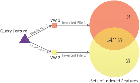
However, the routine of multi-vocabulary merging is affected by a crucial problem, i.e., vocabulary correlation [3] (see Fig. 1). Given a query feature, based on the inverted files with two individual vocabularies, two sets of indexed features and are identified, sharing an intersection set . In this paper, the area of is approximated by . The larger is, the larger the correlation will be. In an extreme case, total correlation occurs if , and merging and brings no benefit.
A straightforward method for multi-vocabulary merging consists in concatenating the BoW histograms of different vocabularies [11]. In a microscopic view of this method, the indexed features in are counted twice in Fig. 1. Nevertheless, since images in this area are mostly irrelevant ones (the number of relevant images is always very small), the over-counting may actually compromise the retrieval accuracy [12].
In this paper, we consider the situation in which the given vocabularies are correlated, and we aim to reduce the impact of correlation. To address this problem, this paper proposes to model the vocabulary correlation problem from a probabilistic view. In a nutshell, we jointly estimate an image- and feature-level similarity for the indexed features in the intersection set (or overlapping area). Given a query feature, lists of indexed features are extracted from multiple inverted files. Then, we identify the intersection and union sets of the lists, from which the cardinality ratio is calculated. This ratio thus encodes the extent of correlation (see Fig. 1). For the indexed images in the intersection set, its similarity with the query is estimated as a function of the cardinality ratio, and subsequently added to the matching score. Experiments on several benchmark datasets demonstrate that Bayes merging is effective, and yields competitive results with the state-of-the-art methods.
2 Related Work
Vocabulary Generation The vocabulary provides a discrete partitioning of the feature space by visual words. Typically, either flat kmeans [12, 4] or hierarchical kmeans [11] is employed to train a vocabulary in an unsupervised manner. Improved methods include incorporating contextual information into the vocabulary [19], building super-sized vocabulary [16, 20, 10], making use of the active points [15], etc.
Matching Refinement Feature-to-feature matching is a key issue in the BoW model. The baseline approach employs a coarse word-to-word matching, resulting in undesirable low precision. To improve precision, some works analyze the spatial contexts [16, 21, 24] of SIFT features, and use the spatial constraints as solution to refining matching. Another line of works extracts binary signatures from SIFT descriptors [4] or its contexts [23, 8]. The feature matching is thus refined by a further check of the Hamming distance between binary signatures. In this paper, however, we argue that even if two features are adjacent in the feature space, the corresponding images are probably very different. Therefore, we are supposed to look one step further by estimating a joint similarity on both image- and feature-level from clues in multiple vocabularies.
Multiple Vocabularies It is well known that multi-vocabulary merging is effective in improving recall [3, 18]. Typically, multi-vocabulary merging can be performed either at score level, e.g., by concatenating the BoW histograms [11], or at rank level, e.g., by rank aggregation [7]. On the other hand, some works also provide clues that multiple vocabularies also improve precision [1, 17]. To address the problem of vocabulary correlation, Xia et al. [18] propose to create the vocabularies jointly and reduce correlation from the view of vocabulary generation. A more relevant work includes [3], which uses PCA to implicitly remove correlation of given vocabularies, resulting in a low dimensional image representation. Our work departs from previous works in two aspects. First, we explicitly model the vocabulary correlation problem from a probabilistic view. Second, our work is proposed for the BoW based image retrieval task, which differs from NN search problems.
3 Background
3.1 Notations
Assume that the vocabularies are denoted as , where represents a visual word and is the vocabulary size. Correspondingly, built on , inverted files are organized as , where each entry contains a list of indexed features.
Given a query SIFT feature , it is quantized to a visual word tuple , where is the nearest centroid in to . With the visual words we can identify sets of indexed features in entries . From the sets, we can define three types of sets to be used in this paper.
Definition 1 (-order intersection set)
The intersection set of , and only sets, denoted as , .
Definition 2 (-order union set)
The union set of , and only sets, denoted as , .
Definition 3 (difference set)
The set in which no overlapping exists, i.e., , .
3.2 Baselines
Single vocabulary baseline (B0) For a single vocabulary, we adopt the baseline introduced in [12, 4]. Specifically, vocabularies are trained by AKM on the independent Flickr60K data [4], and average IDF [22] weighting scheme is used. We replace the original SIFT descriptor with rootSIFT [13]. In this scenario, we denote the matching function between two features and as,
| (1) |
where and are visual words of and in the vocabulary, respectively, and is the Kronecker delta response.
Conventional vocabulary merging (B1) Given vocabularies, B1 simply concatenates multiple BoW histograms [11]. It is equivalent to a simple score-level addition of the outputs of multiple vocabularies. The matching function between features and can be defined as
| (2) |
where and are visual words in vocabulary for and , respectively. Eq. 2 shows that in baseline B1, an indexed feature is counted times if it is in the -order intersection set , and only once if in the difference set (since there is no overlapping).
Multi-index based vocabulary merging (B2) In [1], a multi-index is organized as a multi-dimensional structure. In its nature, given vocabularies, two features are considered as a match iff they are in the -order intersection set of the indexed feature lists. Therefore, in baseline B2, the matching function is defined as
| (3) |
Eq. 3 only counts the indexed features in , discarding the rest. Therefore, the recall is low for B2.
4 Proposed Method
For multi-vocabulary merging, the major problem is the over-counting of the intersection sets . On the other hand, the major benefit is a high recall, which is encoded in the difference set. Taking both issues into consideration, we propose to exert a likelihood on the intersection sets and preserve the difference set (scored as B1). Without loss of generality, we start from the case of two vocabularies and then generalize it to multiple vocabularies.

4.1 Model Formulation
Given a query feature in image , two sets of indexed features and are identified in two inverted files, respectively. Here, we want to evaluate the likelihood that a SIFT feature is a true neighbor of given that belongs to the intersection set of and . This likelihood can be modeled as the following conditional probability,
| (4) |
In Eq. 4, we define as the set of features which are visually similar to (locally) and belong to the ground truth images of (globally). On the other hand, is defined as the features which violate any of the two criteria. Therefore, and satisfy the follows
| (5) |
For simplicity, we denote as , as , and as , Then, using the formula of Bayes’ theorem as well as Eq. 5, we get
| (6) | ||||
Then, re-formulating Eq. 6, we have
| (7) |
In Eq. 7, there are actually three random variables to estimate, i.e., (term 1), (term 2), and (term 3). In Section 4.2, we will exploit the estimation of these probabilities.
4.2 Probability Estimation
Estimation of term 1 In Eq. 7, the term encodes the probability that feature lies in the set given that is a false match of query feature . In this case, we should consider the distribution of the ’ false matches in sets and . In large databases, the number of true matches (both locally and globally) is limited. In other words, false matches dominate the space covered by and . Therefore, we assume that false matches are uniformly distributed in and , and term 1 can be estimated as
| (8) |
where represents the cardinality of a set. Eq. 8 implies that, the probability that a false match falls into is proportional to the cardinality ratio . Intuitively, the larger the intersection set is, the more probable that a false match will fall into it. Fig. 2 depicts the distribution of this cardinality ratio on different database scales.
Estimation of term 2 In contrast to term 1, the probability encoded in term 2 reflects the likelihood that , a true neighbor of query , falls into the intersection set .
Still, we estimate this probability as a function of the cardinality ratio . However, since the number of true matches is very small compared to false ones, we do not adopt the method in estimating term 1. Instead, image data with ground truth is used to analyze the distribution.
Specifically, empirical analysis is performed on Oxford and Holidays datasets. Given a feature in the query image , true matches are defined as the features which have a Hamming distance [4] smaller than to and which appear in the ground truth images of . Then we calculate the ratio of the number of true matches in to the number of true matches in . Finally, the relationship between the ratio and is depicted in Fig. 3.
A surprising fact from Fig. 3 is that increases linearly with . Contrary to our expectation, true matches do not aggregate around the query point. Instead, they tend to scatter in the high-dimensional feature space. Otherwise, the curves in Fig. 3 would take on a -like profile. On the other hand, Fig. 3 also implies that the indexed features in are mostly false matches. This explains why the over-counting compromises the retrieval accuracy. Moreover, we also find that the trend in Fig. 3 seems to be database-independent.

Estimation of term 3 Term 3, i.e., , can be interpreted as the ratio of the probability of being a false match to being a true match. Typically, as the database grows, the number of false images will become larger, and the value of term 3 will increase. To model this property, and thus making our system adjustable to large scale settings, we set term 3 as
| (9) |
where is the number of images in the database, and is a weighting parameter. Note that we add a operator due to numerical considerations.
4.3 Similarity Interpretation
Using the estimation methods introduced in Section. 4.2, we are able to provide an explicit implementation of the probability model (Eq. 4). Specifically, we assume four database sizes are involved, i.e., 5K, 10K, 100K, 1M, and we set the parameter to for better illustration. The derived probability function is plotted against in Fig. 4. From the curves in Fig. 4, we can get several implications in terms of physical interpretation.
First, when the intersection area is very small (the cardinality ratio is close to zero), it is very likely that is a true match if it falls into this area. In this scenario, the discriminative power of the intersection set is high, and can be trusted when merging vocabularies.
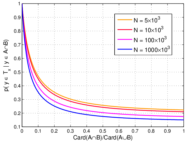
Second, when the cardinality ratio approaches , i.e., sets and share a large overlap, the probability of being a true match is small. This makes more sense if we take into consideration the fact that false images dominate the entire feature space. Moreover, a larger intersection means a larger dependency (or correlation) between two vocabularies, in which situation our method exerts a punishment (low weight) and overcomes this problem to some extent.
Third, as the database becomes larger, the curves lean towards the origin. In fact, for large databases, the chances that is a true match will be more remote under each cardinality ratio. Nevertheless, the cardinality ratio tends to get smaller (see Fig. 2) as the database grows, so the estimated probability will be compensated to some extent.
4.4 Generalization to Multiple Vocabularies
In this section, we generalize our method to the case of multiple vocabularies ().
Given vocabularies, a query feature is quantized to visual words, and subsequently sets of indexed features are identified, i.e., . If a database feature falls into the -order intersection set of , the probability of it being a true match to is defined as
| (10) |
Using the similarity function derived in Section 4.3, we can estimate Eq. 10 as a function of the cardinality ratio of the -order intersection and union sets .
4.5 Proposed Image Retrieval Pipeline
In this section, the matching function of the Bayes merging method is defined as follows,
| (11) |
where is the similarity function defined in Eq. 10. If , Bayes merging reduces to the baseline B1.
The pipeline of Bayes merging is summarized in Algorithm 1. In the offline steps, vocabularies are trained and the corresponding inverted files are organized. During online retrieval, given a query image with descriptors, for each feature , we quantize it to visual words (step 2). Then, lists of indexed features are identified (step 3), from which all -order intersection and union sets are identified (step 4, 5). For each indexed feature in , we find the -order intersection and union sets it falls in (step 7, 8), and calculate the cardinality ratio (step 9). Finally, matching strength is calculated according to Eq. 10 and used in the matching function as Eq. 11 (steps 10 and 11).
For one query feature, we have to traverse twice in Algorithm 1, which doubles the query time. However, in the supplementary material, we demonstrate that we can accomplish this process by traversing only once, thus solving the efficiency problem of Bayes merging.
5 Experiments
In this section, the proposed Bayes merging is evaluated on three benchmark datasets, i.e., Holidays [4], Oxford [12], and Ukbench [11]. The details of the datasets are summarized in Table 1. We also add the Flickr 1M dataset [4] of one million images to test the scalability of our method. All the vocabularies are trained independently on the Flickr60K dataset [4] using AKM [12] with different initial seeds.
| Dataset | # images | # queries | # descriptors | Evaluation |
|---|---|---|---|---|
| Holidays | 1491 | 500 | 4,455,091 | mAP |
| Oxford | 5063 | 55 | 13,516,660 | mAP |
| Ukbench | 10200 | 10200 | 19,415,079 | N-S score |
5.1 Parameter Analysis
One parameter, i.e., the weighting parameter in Eq. 9 is involved in the probabilistic model. We evaluate on the Holidays and Oxford datasets, and record in Table 2 the mAP results against different values of . We can see that the mAP results remain stable when ranges from to , probably due to the effect of the log operator in Eq. 9. We therefore set to in the following experiments.
| Value of in Eq. 9 | 10 | 20 | 30 | 40 | 50 |
|---|---|---|---|---|---|
| Oxford, mAP(%) | 46.72 | 46.80 | 46.77 | 46.73 | 46.73 |
| Holidays, mAP(%) | 58.35 | 58.47 | 58.51 | 58.50 | 58.36 |
5.2 Evaluation


Comparison with the baselines We first compare Bayes merging with the baselines, i.e., , , defined in Section 3.2. The results are demonstrated in Fig. 5 and Fig. 6. From these results we find that baseline does not benefit from introducing multiple vocabularies, and that its performance drops when merging more vocabularies, because the recall further decreases. We speculate that Multiple Assignment will bring benefit [1, 17] to B2. Moreover, baseline B1 brings limited improvements over B0. In fact, B1 has a higher recall than B0, but this benefit is impaired by vocabulary correlation in which many irrelevant images are over-counted.
In comparison, it is clear that Bayes merging yields great improvements. Take Holidays for example, when merging two vocabularies of size 20K, the gains in mAP over the three baselines are , , and , respectively. The improvement is even higher for three vocabularies. Nevertheless, we favor two vocabularies due to the fact that the marginal improvement is prominent, while introducing little computational complexity.
| Methods | Holidays, mAP() | Oxford, mAP() | Ukbench, N-S | ||||||
|---|---|---|---|---|---|---|---|---|---|
| 220K | 320K | 250K | 220K | 320K | 2100K | 220K | 320K | 2100K | |
| 49.23 | 49.23 | 54.17 | 37.80 | 37.80 | 38.80 | 3.11 | 3.11 | 3.17 | |
| 49.87 | 50.49 | 56.64 | 39.78 | 39.97 | 41.28 | 3.15 | 3.16 | 3.22 | |
| Bayes | 58.51 | 60.40 | 59.22 | 46.77 | 49.36 | 49.72 | 3.31 | 3.30 | 3.35 |
| + HE | 77.61 | 78.08 | 77.48 | 58.97 | 59.52 | 60.08 | 3.51 | 3.51 | 3.48 |
| Bayes + HE | 81.20 | 81.56 | 80.60 | 63.32 | 63.53 | 63.96 | 3.61 | 3.62 | 3.57 |
| Bayes + HE + Burst | 81.53 | 81.08 | 65.01 | 64.82 | 64.73 | 3.62 | 3.62 | 3.59 | |
Impact of vocabulary sizes The vocabulary size may have an impact on the effectiveness of Bayes merging. To this end, we generate vocabularies of size 10K, 20K, 50K, 100K, and 200K on the independent Flickr60K data. In Fig. 6, we demonstrate the results obtained from various vocabulary sizes on the three datasets. Except for the three baselines, we also report results obtained by Bayes merging of two or three vocabularies.
From Fig. 6, we can see that B1 still yields limited improvement over B0. Moreover, B1 and B2 perform better under those larger vocabularies. This is due to the fact that larger vocabularies reduce correlation. But for large databases, vocabularies are never large enough, so the correlation problem would be more severe in the large-scale case. Moreover, it is clear that the Bayes merging method exceeds the baselines consistently under different vocabulary sizes. Meanwhile, Bayes merging of three vocabularies has a slightly higher performance than two vocabularies.
Merging vocabularies of different sizes Bayes merging can also be generalized to merging vocabularies of different sizes, and the procedure is essentially the same with Algorithm 1. As with the contribution of each vocabulary, we adopt the same unit weight for all vocabularies, as it is shown to yield satisfying performance in [3]. In this paper, we report the merging results on Oxford dataset in Table 4.
Table 4 demonstrates that merging vocabularies of different sizes marginally improves mAP on Oxford. For example, Bayes merging of two vocabularies of size 10K and 20K improves over the 210K and 220K Bayes methods by and , respectively. We speculate that vocabularies of different sizes provide extra complementary information, which can be captured by our method. However, since the smaller vocabulary introduces more noise, the benefit is limited.
| Method | Bayes | ||
|---|---|---|---|
| 10K + 20K | 40.89 | 32.85 | 47.11 |
| 20K + 50K | 41.20 | 34.70 | 48.85 |
| 10K + 20K + 50K | 42.31 | 35.82 | 49.05 |
Combination with Hamming Embedding To test whether Bayes merging is complementary to some prior arts, we combine it with Hamming Embedding (HE) [4] and burstiness weighting [5] using the default parameters. HE effectively improves the precision of feature matching. In our experiment, HE with a single vocabulary achieves an mAP of and on Holidays and Oxford, and an N-S score of on Ukbench, respectively.
The results in Fig. 5 and Table 3 indicate that Bayes merging yields consistent improvements of the B0 + HE method. Specifically, when merging two vocabularies of 20K, the mAP is improved from to and from to on Holidays and Oxford, respectively. Similar trend can be observed on Ukbench: N-S score rises from 3.49 to 3.61. In its nature, HE results in refined matching in the feature space (locally). Complementarily, the Bayes merging jointly considers the image- and feature-level similarity. Therefore, while good matching in the feature space can be guaranteed by HE, our method punishes those of a false match in the image space. In this scenario, we actually raise an interesting question: can we simply trust feature-to-feature similarity in image retrieval?
In addition, combining burstiness weights brings about extra, though limited improvement (see Table 3). Our implementation differs from [5] in that we do not apply the weights on images in the intersection set, but instead on the difference set () only. A performance summary of various methods is presented in Table 3.
Large-scale experiments To test the scalability of our method, we add the Flickr1M distractor images [4] to the Holidays and Oxford datasets. For comparison, we report the results of baselines and . From Fig. 7, it is clear that Bayes merging outperforms the two baselines significantly. On Holidays dataset mixed with one million images, Bayes merging achieves mAP of 39.60, compared with 28.19 and 29.26 of baseline B0 and B1, respectively.
In terms of efficiency, the baseline method consumes 4 bytes per feature, and 1.9 GB for indexing one million images. The Bayes merging of two vocabularies doubles the memory cost to about 3.8 GB on Flickr1M.
On the other hand, it takes 2.52s and 4.87s for and to perform one query on 1 million image size, respectively, using a server with 3.46 GHz and 64GB memory. Bayes merging involves identifying the intersection set and calculate the cardinality ratio. In fact, the cardinality ratio can be computed and stored offline. Moreover, as shown in the supplementary material, we are able to perform both the identification and the voting tasks by traversing the two lists of indexed features only once. Therefore, our method only marginally increases the query time to 5.12s.

Comparison with state-of-the-arts We first compare our method with [3] which employs PCA to addresses the correlation problem implicitly. In [3], merging four 16K vocabularies and eight 8K vocabularies yield an mAP of and , respectively. Moreover, merging vocabularies of multiple sizes obtains a best mAP of on Holidays. In comparison, the result obtained by Bayes merging is and for two and three vocabularies of size 20K, respectively.
Second, we compare the Bayes merging with the Rank Aggregation (RA) method [2, 7] in Table 5. Following [7], we take the median of multiple ranks as the final rank. Since RA works on the rank level, it does not address the correlation problem, so its performance is limited. The results demonstrate the superiority of Bayes merging.
Finally, we compare the results of Bayes merging with state-of-the-arts in Table 6. On the three datasets, we achive mAP = on Holidays, mAP = on Oxford, and N-S = on Ukbench. We have also tested on the data provided by [14], where the codebook size is 65K. On Oxford datastet, the mAP is 77.3%. Note that some sophisticated techniques are absent in our system, such as spatial constraints [6, 16], semantic consistency [20], etc. Still, the results demonstrate that the performance of Bayes merging is very competitive. We also provide some sample retrieval results in the supplementary material.
| Method | Bayes | Rank aggregation | ||||
|---|---|---|---|---|---|---|
| # vocabularies | 2 | 3 | 3 | 5 | 7 | 9 |
| Holidays, mAP(%) | 58.5 | 60.4 | 49.9 | 50.7 | 51.0 | 51.0 |
| Oxford, mAP(%) | 46.8 | 49.4 | 39.5 | 40.8 | 41.2 | 41.4 |
6 Conclusion
Multi-vocabulary merging is an effective method to improve the recall of visual matching. However, this process is impaired by vocabulary correlation. To address the problem, this paper proposes a Bayes merging approach to explicitly estimate the matching strength of the indexed features in the intersection sets, while preserving those in the difference set. In a probabilistic view, Bayes merging is capable of jointly modeling an image- and feature-level similarity from multiple sets of indexed features. Specifically, we exploit the probability that an indexed feature is a true match (both locally and globally) if it is located in the intersection sets of multiple inverted files. Extensive experiments demonstrate that Bayes merging effectively reduces the impact of vocabulary correlation, thus improving the retrieval accuracy significantly. Further, our method is efficient, and yields competitive results with state-of-the-arts.
Acknowledgement This work was supported by the National High Technology Research and Development Program of China (863 program) under Grant No. 2012AA011004 and the National Science and Technology Support Program under Grant No. 2013BAK02B04. This work also was supported in part to Dr. Qi Tian by ARO grant W911NF-12-1-0057, Faculty Research Awards by NEC Laboratories of America, and 2012 UTSA START-R Research Award respectively. This work was supported in part by National Science Foundation of China (NSFC) 61128007.
References
- [1] A. Babenko and V. Lempitsky. The inverted multi-index. In CVPR, 2012.
- [2] R. Fagin, R. Kumar, and D. Sivakumar. Efficient similarity search and classification via rank aggregation. In ACM SIGMOD, 2003.
- [3] H. Jégou and O. Chum. Negative evidences and co-occurences in image retrieval: The benefit of pca and whitening. In ECCV. 2012.
- [4] H. Jégou, M. Douze, and C. Schmid. Hamming embedding and weak geometric consistency for large scale image search. In ECCV, 2008.
- [5] H. Jégou, M. Douze, and C. Schmid. On the burstiness of visual elements. In CVPR, 2009.
- [6] H. Jégou, M. Douze, and C. Schmid. Improving bag-of-features for large scale image search. IJCV, 2010.
- [7] H. Jegou, C. Schmid, H. Harzallah, and J. Verbeek. Accurate image search using the contextual dissimilarity measure. PAMI, 32(1):2–11, 2010.
- [8] Z. Liu, H. Li, W. Zhou, R. Zhao, and Q. Tian. Contextual hashing for large-scale image search. TIP, 23(4):1606–1614, 2014.
- [9] D. G. Lowe. Distinctive image features from scale invariant keypoints. IJCV, 2004.
- [10] A. Mikulík, M. Perdoch, O. Chum, and J. Matas. Learning a fine vocabulary. In ECCV. 2010.
- [11] D. Niester and H. Stewenius. Scalable recognition with a vocabulary tree. In CVPR, 2006.
- [12] J. Philbin, O. Chum, M. Isard, and A. Zisserman. Object retrieval with large vocabularies and fast spatial matching. In CVPR, 2007.
- [13] A. Relja and A. Zisserman. Three things everyone should know to improve object retrieval. In CVPR, 2012.
- [14] G. Tolias, Y. Avrithis, and H. Jégou. To aggregate or not to aggregate: Selective match kernels for image search. In ICCV, 2013.
- [15] J. Wang, J. Wang, Q. Ke, G. Zeng, and S. Li. Fast approximate k-means via cluster closures. In CVPR, 2012.
- [16] X. Wang, M. Yang, T. Cour, S. Zhu, K. Yu, and T. X. Han. Contextual weighting for vocabulary tree based image retrieval. In ICCV, 2011.
- [17] Z. Wu, Q. Ke, J. Sun, and H.-Y. Shum. A multi-sample, multi-tree approach to bag-of-words image representation for image retrieval. In CVPR, 2009.
- [18] Y. Xia, K. He, F. Wen, and J. Sun. Joint inverted index. In ICCV, 2013.
- [19] S. Zhang, Q. Huang, G. Hua, S. Jiang, W. Gao, and Q. Tian. Building contextual visual vocabulary for large-scale image applications. In ACM MM, 2010.
- [20] S. Zhang, M. Yang, X. Wang, Y. Lin, and Q. Tian. Semantic-aware co-indexing for near-duplicate image retrieval. In ICCV, 2013.
- [21] L. Zheng and S. Wang. Visual phraselet: Refining spatial constraints for large scale image search. Signal Processing Letters, IEEE, 20(4):391–394, 2013.
- [22] L. Zheng, S. Wang, Z. Liu, and Q. Tian. Lp-norm idf for large scale image search. In CVPR, 2013.
- [23] L. Zheng, S. Wang, Z. Liu, and Q. Tian. Packing and padding: Coupled multi-index for accurate image retrieval. In CVPR, 2014.
- [24] W. Zhou, H. Li, Y. Lu, and Q. Tian. Principal visual word discovery for automatic license plate detection. TIP, 21(9):4269–4279, 2012.