Lighting up topological insulators: large surface photocurrents from magnetic superlattices

Light-matter interactions are central to modern science and technology. It is the principle at the heart of many solid-state material probes, and at the same time, it is an important ingredient in our energy economy, particularly through photovoltaic harvesting of solar energy. A challenging problem of solar energy is how to harness the infrared (IR) part of the spectrum. This could apply to the solar radiation, as well as to Earth’s radiation, which is almost exclusively in the infrared, and continuously has the same energy flux as the sun [1]. Similarly, electric mid and far infrared detection is essentially limited to a single type of material: HgCdTe alloys. Additional platforms are likely to be competitive in certain temperature and frequency regimes.

Efforts to extend the spectrum accessible in photovoltaics concentrated on new low band-gap materials; organics [2, 3, 4, 5], as well as carbon nanotubes [6, 7, 8] were shown capable of IR harvesting, albeit with a small efficiency. Another approach utilizes plasmonics as an intermediate step between IR and currents in a semiconductor [9, 10, 11, 12].

When mentioning new materials for IR harversting, topological insulators [13, 14, 15, 16, 17] immediately come to mind. On the one hand, they have a unique response to electromagnetic fields [18, 19, 20]. More importantly, their mid-gap surface states exhibiting spin-momentum locking raised hopes that surface photocurrents could easily be produce by irradiation with circularly-polarized light. These hopes have gone unfulfilled. Even when including a series of modifications to the band structure likely to appear in real materials, such as warping, band curvature, or a uniform magnetic field, the photocurrents produced in response to sub-bandgap light were shown to be remarkably minute, even when a high-intensity laser is considered [21, 22]. The only scheme for producing a photo-voltage so far relied on the unique thermoelectric effects associated with a Dirac cone dispersion [23].

In this manuscript we describe how to turn a topological insulator surface with a simple Dirac dispersion into a photocurrent rectifier. We show that by adding a magnetic coating with a spatially periodic magnetic texture, the TI produces a significant surface photocurrent in response to circularly polarized light in the IR regime. This effect should, in principle, allow making diode-free IR sensitive photocells from topological insulator films. We discuss application of the effect to room temperature infra-red detection, and show that it can lead to a detector operating at much larger wavelengths then those available with existing technologies. Beyond such applications, the effect can be used to investigate the unique properties of TI surfaces using non-ionizing light (as in [24]).

The paper is organized as follows. In Sec. II, we give a description of the device and summarize our main results. In Sec. III we present the model describing the magnetically patterned TI surface. The symmetries of the model are discussed in Sec. IV. In Sec. V we derive the equations describing the photocurrent response of the device. We consider the implications of the symmetries on the photocurrent response (Sec. V.1), and find the conditions under which a large photocurrent response is obtained. A perturbative calculation of the photocurrent response is given in Sec. V.2. Our main results for the frequency dependent photocurrent response of the device are given in Sec. VI. Several applications of the device, and in particular, room temperature infra-red detection are discussed in Sec. VII. We close with concluding remarks in Sec. VIII.

The device we propose and analyze in this paper consists of a bulk three dimensional topological insulator, whose surface is coated with stripes of magnetic material, see Fig. 1. We consider magnetic stripes which are evenly spaced. The stripes’ spacing defines a wave vector ${\bf q}$ in the plane of the surface and normal to the orientation of the stripes. Via their magnetic coupling to the electrons in the surface state of the TI, the magnetic stripes break symmetries which suppress the photocurrents in their absence. Thereby, the magnetic stripes dramatically enhance the photocurrent response of the TI’s surface. The magnetic stripes are taken to be magnetically ordered in the same direction. As we explain in Sec. IV, the direction of the stripes’ magnetization needs to have non-zero components both normal to the surface as well as along the vector ${\bf q}$. The photocurrents flow parallel to the direction of the stripes (perpendicular to ${\bf q}$), as shown in Sec. IV.

The photocurrent response of the device can be described by a dimensionless, frequency dependent response function $\eta(\omega)$. In Sec. VI we demonstrate a key feature of $\eta(\omega)$: it exhibits a strong maximum at frequency $\omega\approx 1.7v_{F}|{\bf q}|$, where $v_{F}$ is the velocity associated the Dirac cone. This result has significant implications in future applications of the proposed device: the frequency corresponding to the peak sensitivity of the device can be tuned by appropriately choosing the spacing of the magnetic stripes. In Sec. VI.1, we analyze the performance of this set-up at finite temperature and with the chemical potential tuned away from the Dirac point. This analysis gives an “operational” region for the device: we show that the performance of the device is not significantly reduced for temperatures up to $\hbar v_{F}|{\bf q}|$, which could translate to $300K$ in practical realizations. Similarity, we show that deviations of the chemical potential from the Dirac point do not significantly hinder the the performance, as long as they remain below $\hbar v_{F}|{\bf q}|$.

Quantitative estimates for the photocurrent response in several applications are given in Sec. VII. We estimate that the two dimensional photocurrent density resulting from illumination with sunlight could reach $10^{-8}\frac{A}{m}$. Illumination with a conventional laser beam can yield currents of the order of $10^{-4}\frac{A}{m}$. A particularly appealing application of the device is room temperature detection of infra-red radiation. We explore the potential of this system to detect black-body radiation emitted at a variety of different source temperatures. We conclude that the device may be able to detect black-body radiation of objects at room temperature while itself being at a comparable temperature. Finally, we explore several theoretical figures of merit for the device as a room temperature IR detector. In particular we calculate the device’s external quantum efficiency and its specific detectivity, which gives its normalized signal to noise ratio [25] . Near room temperature and with peak sensitivity tuned to wavelengths near $15\mu$m we estimate a quantum efficiency of 0.01$\%$ and a specific detectivity $\sim 10^{7}$ cm$\sqrt{\text{Hz}}$/W, before any device optimization takes place. Such a detectivity compares well with the detectivity of current room temperature photo-detectors [26], which can usually only detect up to $10\mu\mathrm{m}$ [27, 28, 29, 26, 30, 31]. Importantly, the proposed device has the potential to be functional for wavelengths greater than $15\mu\mathrm{m}$. Our findings therefore support the idea that this set-up may be promising for room temperature detection of long wavelength infrared radiation.

Our photocurrent rectification scheme emerges from the minimal model of a surface of a 3D topological insulator (TI). With the surface lying in the $xy$ plane, the Hamiltonian describing the surface electrons is

$\displaystyle H_{0}$

$\displaystyle=$

$\displaystyle v_{F}\left(p_{x}\sigma^{y}-p_{y}\sigma^{x}\right),$

(1)

where $\sigma^{x},\sigma^{y}$ are Pauli matrices, and $\mathbf{p}=(p_{x},p_{y})=\left(\frac{\hbar}{i}\frac{\partial}{\partial x},\,\frac{\hbar}{i}\frac{\partial}{\partial y}\right)$. This model is clearly time-reversal and rotationally invariant, ${\cal T}H_{0}{\cal T}^{-1}=U_{\phi}H_{0}U_{\phi}^{\dagger}=H_{0}$, with the symmetry operators

$${\cal T}=i\sigma_{y}K,\hskip 28.45274ptU_{\phi}=e^{i\phi\left(\sigma^{z}/2+L_{z}/\hbar\right)}.$$

(2)

Here, $K$ denotes complex conjugation, $L_{z}=xp_{y}-yp_{x}$ is the orbital angular momentum normal to the surface, and $\phi$ the angle of rotation.

These two symmetries immediately imply no current response to incident light at normal incidence. Time-reversal invariance requires that the incident beam is circularly polarized to see any response. Since circularly polarized light, however, has no preferred direction on the surface, the rotational symmetry rules out any net photocurrent from forming. In materials such as $\mathrm{Bi_{3}Se}_{2}$, the lattice structure reduces the full $SO(2)$ rotational symmetry to a $C_{3}$ symmetry, with $\phi=2\pi/3$ in Eq. (2). This allows $H_{0}$ to have a trigonal warping term [32]. However even with the reduced symmetry, no photocurrents are possible [21, 22].

Next, we consider a magnetic grating structure deposited on the surface, see Fig. 1. Consider strips of a ferromagnetic material set parallel to the $y$ axis, and placed periodically with a wave number $\mathbf{q}=(q,0)$. We model the proximity-induced ferromagnetic interaction on the surface electrons by

$$V=\mathbf{u}\cdot{\mbox{\boldmath$\sigma$}}\cos(qx).$$

(3)

Once the magnetic structure is introduced, it is convenient to enumerate the eigenstates of the full Hamiltonian, $H=H_{0}+V$ within the reduced Brillouin zone (BZ) in terms of the quasi-momentum $k_{x}\in[-\frac{q}{2},\frac{q}{2}]$ in x-direction, using Greek indices to denote the bands. Thus denote the eigenstates as $\left|k_{x},k_{y};\alpha\right>$. We use the convention that conduction bands are enumerated by $\alpha>0$ and valence bands by $\alpha<0$, as illustrated in Fig. 2

The addition of the magnetic strips on the surface alters its symmetries. Time-reversal symmetry remains, as long as we consider a modified operator which concatenates time reversal with a spatial translation: $\tilde{\cal T}={\cal T}M$ with $MxM^{\dagger}=x+\pi/q$. The eigenstates and energies transform as

$$\left|-k_{x},-k_{y};\alpha\right>=\tilde{\cal T}\left|k_{x},k_{y};\alpha\right>,E_{-k_{x},-k_{y};\alpha}=E_{k_{x},k_{y};\alpha}$$

(4)

Particle-hole symmetry is also present. First define $\Pi_{a}$ as the spatial reflection operator about the $a=x,y$ directions, e.g., $\Pi_{x}x\Pi_{x}=-x$. Now, ${\cal C}=\Pi_{x}\Pi_{y}{\cal T}$ implements:

$$\left|k_{x},k_{y};-\alpha\right>={\cal C}\left|k_{x},k_{y};\alpha\right>,E_{k_{x},k_{y};\alpha}=-E_{k_{x},k_{y};-\alpha}.$$

(5)

Additional symmetries appear restricted due to the arbitrary form of $V$.

Nonetheless, a gauge transformation allows us to cancel an arbitrary $u_{y}$ component of $V$, and allows additional mirror symmetries. Define the gauge transformation

$$G=\exp{\left(i\frac{u_{y}}{\hbar v_{F}q}\sin qx\right)}.$$

(6)

It is easy to verify that

	$\displaystyle\tilde{H}=GHG^{-1}$	$\displaystyle=$	$\displaystyle H-u_{y}\sigma^{y}\cos qx$		(7)
		$\displaystyle=$	$\displaystyle H_{0}+(u_{x}\sigma^{x}+u_{z}\sigma^{z})\cos qx.$

With $u_{y}$ eliminated, we can construct the mirror transformation

$${\cal P}_{x}=\Pi_{y}K.$$

(8)

The only term that can possibly be affected by this compounded transformation is actually invariant,

$$\begin{array}[]{c}\Pi_{y}K\l[\frac{\hbar v_{F}}{i}\l(-\sigma^{x}\partial_{y})]K^{-1}\Pi_{y}\\ =\Pi_{y}\l[\frac{\hbar v_{F}}{i}\l(\sigma^{x}\partial_{y})]\Pi_{y}=\frac{\hbar v_{F}}{i}\l(-\sigma^{x}\partial_{y}),\end{array}$$

(9)

so that ${\cal P}_{x}\tilde{H}{\cal P}_{x}^{-1}=\tilde{H}$. Since complex conjugation imposes $(k_{x},k_{y})\rightarrow(-k_{x},-k_{y})$, and $\Pi_{y}$ reverses $-k_{y}$ back to $k_{y}$, we have:

$$\left|-k_{x},k_{y};\alpha\right>={\cal P}_{x}\left|k_{x},k_{y};\alpha\right>,E_{-k_{x},k_{y};\alpha}=E_{k_{x},k_{y};\alpha}.$$

(10)

By compounding ${\cal P}_{x}$ with time reversal, $\tilde{\cal T}$, we also obtain a reflection about the x-axis: $\tilde{\cal T}{\cal P}_{x}:(k_{x},k_{y})\rightarrow(k_{x},-k_{y})$. Below we will first discuss the equations describing the photocurrent response of the device, and then consider the consequences of the symmetries on the resulting photocurrent.

Within Fermi’s golden rule, we expect that the photocurrent response to a particular frequency will be quadratic in the photon field. We restrict ourselves to normally incident photons, at frequencies which allow us to approximate the vector potential as spatially uniform, $\mathbf{A}(\mathbf{x},t)={\rm Re}\mathbf{A}_{0}(\omega)e^{i\omega t}$. Then, the $k,m,n=x,y$ component of the photocurrent is quite generally given by:

$$j_{k}(\omega)=\frac{e\tau}{4\hbar\omega^{2}}E_{m}(\omega){\cal Q}_{kmn}(\mathbf{\omega})E_{n}^{*}(\omega).$$

(11)

Here, repeated indices are summed, ${\bf E}(\omega)=-i\omega{\bf A_{0}}$. Also, in Eq. (11) we assume that the current decays on a time scale $\tau$. Quite remarkably, in the presence of a periodic structure of magnetic strips lying along the y-axis, we will find that there is only one independent element of ${\cal Q}_{kmn}(\mathbf{\omega})$ which is nonzero:

$${\cal Q}(\omega)_{y,x,y}={\cal Q}(\omega)_{y,y,x}^{*}=-{\cal Q}(\omega)_{y,y,x}.$$

To calculate ${\cal Q}_{kmn}(\mathbf{\omega})$, we first write the surface photon-electron interaction, which we assume follows the minimal coupling prescription:

$$\hat{H}_{int}=e\frac{\partial H_{0}}{\partial\mathbf{p}}\cdot\mathbf{A}(\mathrm{\mathbf{x}},t).$$

(12)

The presence of the photon field can either excite electrons to a higher sub band or allow them to relax to a lower sub band through emission. Taking these possibilities into account we have the following result for ${\cal Q}_{kmn}(\omega)$

$${\cal Q}_{kmn}(\omega)=\int\frac{d^{2}k}{(2\pi)^{2}}\sum_{\alpha,\beta}{\cal Q}_{kmn}^{\alpha\beta}(\mathbf{k},\omega,T,\mu),$$

(13)

where ${\cal Q}_{kmn}^{\alpha\beta}(\mathbf{k},\omega,T,\mu)$ describes the excitation/relaxation of electrons at momentum $\mathbf{k}$ and temperature $T$. An application of Fermi’s golden rule yields:

$$\begin{array}[]{c}{\cal Q}_{kmn}^{\alpha\beta}(\mathbf{k,\omega},T,\mu)={\hat{\mathbf{x}}_{k}}\cdot\left(\mathbf{v}_{\mathbf{k}}^{(\alpha)}-\mathbf{v_{k}^{(\beta)}}\right)M_{mn}^{\alpha\beta}(\mathbf{k})\\ \times 2\pi\mathrm{\delta(E_{\mathbf{k}}^{(\alpha)}-E_{\mathbf{k}}^{(\beta)}-\omega)}(n^{0}_{\mathbf{k},\beta}-n^{0}_{\mathbf{k},\alpha}),\end{array}$$

(14)

where $n^{0}_{\mathbf{k},\beta}$ is a Fermi function at a temperature $T$ and chemical potential $\mu$ and the velocities in the band $\alpha$ are given by $\mathbf{v}_{\mathbf{k}}^{(\alpha)}=\left<\mathbf{k};\alpha\right|\frac{\partial H_{0}}{\partial\mathbf{p}}\left|\mathbf{k};\alpha\right>$, and the matrix elements are given by

$$M_{mn}^{\alpha\beta}(\mathbf{k})=\left<\mathbf{k},\alpha\right|\Gamma_{m}\left|\mathbf{k},\beta\right>\left<\mathbf{k},\beta\right|\Gamma_{n}^{\dagger}\left|\mathbf{k},\alpha\right>,$$

(15)

with $\Gamma_{m}=e\frac{\partial H_{0}}{\partial\mathbf{p}}\cdot\hat{\mathbf{x}}_{m}$. From this definition it is clear that $M_{mn}^{\alpha\beta}(\mathbf{k})=\left(M_{nm}^{\alpha\beta}(\mathbf{k})\right)^{*}$, i.e., it is hermitian. At zero temperature and with the chemical potential tuned to the Dirac point the valance sub bands are entirely full and the conduction sub bands completely empty. In this case only electron excitation is possible and we may excite electrons from any sub band of the valence band to any sub band of the conduction band, and at any momentum. Therefore:

$${\cal Q}_{kmn}(\omega)=\int\frac{d^{2}k}{(2\pi)^{2}}\sum_{\alpha>0,\beta<0}{\cal Q}_{kmn}^{\alpha\beta}(\mathbf{k},\omega),$$

(16)

where ${\cal Q}_{kmn}^{\alpha\beta}(\mathbf{k},\omega)={\cal Q}_{kmn}^{\alpha\beta}(\mathbf{k,\omega},T\to 0,\mu=0)$ accounts for excitations from the valence band $\beta<0$ to the conduction band $\alpha>0$ at momentum $\mathbf{k}$. It is this limiting case that we will develop first, and then move on to discuss how temperature and chemical potential effect these results. Setting $T\to 0$ and $\mu=0$ in Eq. (14) now gives

$$\begin{array}[]{c}{\cal Q}_{kmn}^{\alpha\beta}(\mathbf{k,\omega})={\hat{\mathbf{x}}_{k}}\cdot\left(\mathbf{v}_{\mathbf{k}}^{(\alpha)}-\mathbf{v_{k}^{(\beta)}}\right)M_{mn}^{\alpha\beta}(\mathbf{k})\\ \times 2\pi\mathrm{\delta(E_{\mathbf{k}}^{(\alpha)}-E_{\mathbf{k}}^{(\beta)}-\omega)},\end{array}$$

(17)

Our results are best expressed in terms of the intensity, $I$, of the light field. For a coherent monochromatic circularly polarized wave with electric-field amplitude $E_{0}$, we have $I=\epsilon_{0}cE_{0}^{2}$. This yields the current response:

$$j_{y}(\omega)=\frac{e^{3}v_{F}^{2}q\tau}{\epsilon_{0}c\hbar^{2}}\frac{I}{\omega^{2}}\eta(\omega)$$

(24)

in terms of the dimensionless frequency-dependent response, $\eta(\omega)$, defined by ${\cal Q}_{yxy}(\omega)=2\frac{e^{2}v_{F}^{2}q}{\hbar}\eta(\omega)$. For a continuous spectrum with intensity per unit angular frequency, containing both circular polarizations, we write $I(\omega)d\omega=2\epsilon_{0}c|{\bf E}(\omega)|^{2}$. The total current response is then:

$$j_{y}=\frac{e^{3}v_{F}^{2}q\tau}{2\epsilon_{0}c\hbar^{2}}\int\limits_{0}^{\Omega}\frac{I(\omega)}{\omega^{2}}\eta(\omega)d\omega,$$

(25)

where $\Omega$ is the high-frequency cutoff.

Fig. 3 displays our numerical results for the dimensionless response $\eta(\omega)$ for three magnetic patterning strengths. We make three observations: (1) Most of the contribution to the current density arises from frequencies $\omega>v_{F}q$. (2) For $\omega\gg v_{F}q$, the dimensionless response $\eta(\omega)$ approaches a constant. (3) $\eta(\omega)$ changes sign at $\Omega^{*}\sim v_{F}q$. The latter observation can also be deduced from Eq. (23), as $F_{0}(\mathbf{k})$ differs in sign from the two other contributions, and dominates below $\Omega^{*}$.

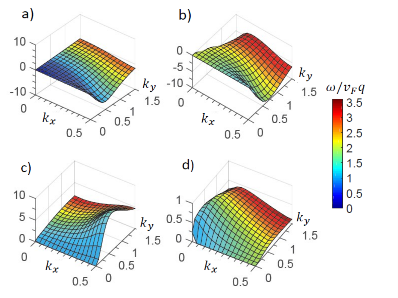
Further intuition for the origin of the photocurrent distributions can be gained by studying the momentum-specific response $\tilde{{\cal Q}}_{yxy}^{\alpha\beta}(\mathbf{k},\omega)$. These are plotted in Fig. 6 of the appendix, which demonstrates that the momenta contributing to the photocurrent are uniformly distributed in the reduced BZ. Furthermore, in agreement with the perturbative results, the sign change of $\eta(\omega)$ is shown to arise due to processes involving scattering by momentum $\pm{\bf q}$ (indicated in red and blue in Fig. 2) which dominate for $\omega>\Omega^{*}$; they contribute with opposite sign to momentum conserving processes (green and purple in Fig. 2), which dominate at low frequencies.

Here we outline several appealing practical aspects of this device. We begin by calculating some representative photocurrents for the illumination of the device by particular radiation sources. We move on to discuss the “tunability" of the device with $q$ and consider its application to room temperature black body detection. We close with a theoretical treatment of the figures of merit for the device as a room temperature IR detector. We show that at room temperature, the normalized signal to noise ratio (specific detectivity) is comparable with present technologies. Importantly, the device can achieve this signal to noise ratio for wavelengths which go beyond those accessible for current technologies.

The unique properties of the surfaces of topological insulators beg to be translated into practical applications. The lack of a generic photocurrent response on such surfaces so far has stifled the possibility of applications in light detection and photovoltaics. In this manuscript we demonstrated how surface magnetic patterning employs the spin-orbit locking, and allows for a substantial photocurrent response even to low-intensity sources such as the low-energy solar spectrum. The surface is naturally sensitive to photon energies below the bandgap of $0.3eV$, as opposed to semiconductor based photovoltaics, which require energies that exceed the material’s bandgap. As such, this effect can be used for detection of micrometer wavelength radiation - a range with limited electric detection schemes. Our estimates give a specific detectivity of $\sim 10^{7}$ cm$\sqrt{\text{Hz}}$/W at $15\mu$m and room temperature, with the ability to go to higher wavelengths by adjusting the separation between magnetic strips. This value of the specific detectivity has room for further optimization by, e.g. creating a layered device. Present technologies with comparable room temperature detectivities are confined to wavelengths $\leq 10\mu$m and therefore the proposed device represents a significant potential advancement in mid-IR and far-IR detection. We note that magnetic coating of topological insulators has been experimentally demonstrated in refs. [46, 47, 48], as well as studied numerically using first principle calculations [49]. The use of magnetic insulators, such as the ones used in [48], will be advantageous in order to minimize effects such as absorption by the magnetic coating and electron doping of the TI surface.

Many aspects remain unexplored. To understand how the TI surface could be harnessed for solar energy harvesting, we need to understand what the natural open-circuit voltage is. In addition, we have only provided a crude account of disorder and phonon scattering effects on the surface, and completely ignored the possibility of bulk contributions at high frequencies. Lastly, we are confident that the magnitude of the effect could be improved by optimizing our device by using other magnetic patterns, or different materials. For instance, we expect that a similar affect will exist in arrays of 2d topological insulator strips, e.g., HgTe/CdTe heterostructures, put in an in-plane spatially varying field. We intend to explore at least some of these issues in future work.

We acknowledge financial support from NSF through DMR-1410435, the Packard Foundation, the IQIM - an NSF center funded in part by the Gordon and Betty Moore Foundation - and especially DARPA through FENA (Caltech), through SPP 1666 of the Deutsche Forschungsgemeinschaft and the Helmholtz Virtual Institute “New States of Matter and Their Excitations” (Berlin). NL acknowledges support from the CIG Marie Curie grant, the Bi-National Science Foundation and I-Core: the Israeli Excellence Center "Circle of Light" (Technion). AF acknowledges support from the Natural Sciences and Engineering Research Council of Canada through the Vanier Canada Graduate Scholarships program and McGill HPC supercomputing resources. Finally, GR and FvO acknowledge the hospitality of the Aspen Center for Physics where a portion of this work was completed.

References

- [1] S. J. Byrnes, R. Blanchard, and F. Capasso, Proceedings of the National Academy of Sciences 111, 3927 (2014).
- [2] D. Muhlbacher, M. Scharber, M. Morana, Z. Zhu, D. Waller, R. Gaudiana, and C. Brabec, Advanced Materials 18, 2884 (2006).
- [3] B. Evaand and F. C. Krebs, Solar Energy Materials and Solar Cells 91, 954 (2007).
- [4] S. H. Park, A. Roy, S. Beaupre, S. Cho, N. Coates, J. S. Moon, D. Moses, M. Leclerc, K. Lee, and A. J. Heeger, Nature Photonics 3, 297 (2009).
- [5] R. R. Lunt and V. Bulovic, Applied Physics Letters 98, 113305 (2011).
- [6] H. Ago, K. Petritsch, M. S. P. Shaffer, A. H. Windle, and R. H. Friend, Advanced Materials 11, 1281 (1999).
- [7] E. Kymakis and G. A. J. Amaratunga, Applied Physics Letters 80, 112 (2002).
- [8] R. M. Jain, R. Howden, K. Tvrdy, S. Shimizu, A. J. Hilmer, T. P. McNicholas, K. K. Gleason, and M. S. Strano, Advanced Materials 24, 4436 (2012).
- [9] H. A. Atwater and A. Polman, Nature Materials 9, 205 (2010).
- [10] M. T. Sheldon and H. A. Atwater, arXiv:1202.0301 .
- [11] K. Nakayama, K. Tanabe, and H. A. Atwater, Applied Physics Letters 93, 121904 (2008).
- [12] E. Briones, J. Briones, J. C. Martinez-Anton, A. Cuadrado, S. McMurtry, M. Hehn, F. Montaigne, J. Alda, and J. González, arXiv preprint arXiv:1412.2658 (2014).
- [13] L. Fu, C. L. Kane, and E. J. Mele, Phys. Rev. Lett. 98, 106803 (2007).
- [14] H. Zhang, C.-X. Liu, X.-L. Qi, X. Dai, Z. Fang, and S.-C. Zhang, Nat Phys 5, 438 (2009).
- [15] J. E. Moore and L. Balents, Phys. Rev. B 75, 121306 (2007).
- [16] D. Hsieh, D. Qian, L. Wray, Y. Xia, Y. S. Hor, R. J. Cava, and M. Z. Hasan, Nature 452, 970 (2008).
- [17] Y. Xia, D. Qian, D. Hsieh, L. Wray, A. Pal, H. Lin, A. Bansil, D. Grauer, Y. S. Hor, R. J. Cava, and M. Z. Hasan, Nat Phys 5, 398 (2009).
- [18] X.-L. Qi, T. L. Hughes, and S.-C. Zhang, Phys. Rev. B 78, 195424 (2008).
- [19] X.-L. Qi, R. Li, J. Zang, and S.-C. Zhang, Science 323, 1184 (2009).
- [20] A. M. Essin, J. E. Moore, and D. Vanderbilt, Physical Review Letters 102, 146805 (2009).
- [21] P. Hosur, Phys. Rev. B 83, 035309 (2011).
- [22] A. Junck, G. Refael, and F. von Oppen, Phys. Rev. B 88, 075144 (2013).
- [23] N. M. Gabor, J. C. W. Song, Q. Ma, N. L. Nair, T. Taychatanapat, K. Watanabe, T. Taniguchi, L. S. Levitov, and P. Jarillo-Herrero, Science 334, 648 (2011).
- [24] J.W. McIver, D. Hsieh, H. Steinberg, P. Jarillo-Herrero, and N. Gedik, Nat. Nanotech. 7, 96 (2011).
- [25] A. Rogalski, Progress in quantum electronics 27, 59 (2003).
- [26] Z. Zhu, S. Joshi, and G. Moddel, Selected Topics in Quantum Electronics, IEEE Journal of 20, 70 (2014).
- [27] E. García-Hemme, R. García-Hernansanz, J. Olea, D. Pastor, A. del Prado, I. Mártil, and G. González-Díaz, Applied Physics Letters 104, 211105 (2014).
- [28] S.-F. Tang, S.-Y. Lin, and S.-C. Lee, Applied Physics Letters 78, 2428 (2001).
- [29] L. Zhou, Y. Zhang, X. Chen, Y. Gu, H. Li, Y. Cao, and S. Xi, Journal of Physics D: Applied Physics 47, 085107 (2014).
- [30] J. Piotrowski, M. Grudzien, Z. Nowak, Z. Orman, J. Pawluczyk, M. Romanis, and W. Gawron, in International Symposium on Optical Science and Technology (International Society for Optics and Photonics, 2000) pp. 175–184.
- [31] H. W. Shin, S. J. Lee, D. G. Kim, M.-H. Bae, J. Heo, K. J. Choi, W. J. Choi, J.-w. Choe, and J. C. Shin, Scientific reports 5 (2015).
- [32] L. Fu, Phys. Rev. Lett. 103, 266801 (2009).
- [33] N. Kumar, B. A. Ruzicka, N. P. Butch, P. Syers, K. Kirshenbaum, J. Paglione, and H. Zhao, Phys. Rev. B 83, 235306 (2011).
- [34] J. Qi, X. Chen, W. Yu, P. Cadden-Zimansky, D. Smirnov, N. H. Tolk, I. Miotkowski, H. Cao, Y. P. Chen, Y. Wu, S. Qiao, and Z. Jiang, Applied Physics Letters 97, 182102 (2010).
- [35] R. C. Hatch, M. Bianchi, D. Guan, S. Bao, J. Mi, B. B. Iversen, L. Nilsson, L. Hornekær, and P. Hofmann, Phys. Rev. B 83, 241303 (2011).
- [36] Z.-H. Pan, A. V. Fedorov, D. Gardner, Y. S. Lee, S. Chu, and T. Valla, Phys. Rev. Lett. 108, 187001 (2012).
- [37] S. Giraud, A. Kundu, and R. Egger, Phys. Rev. B 85, 035441 (2012).
- [38] G. Q. Huang, EPL 100, 17001 (2012).
- [39] C. Chen, Z. Xie, Y. Feng, H. Yi, A. Liang, S. He, D. Mou, J. He, Y. Peng, X. Liu, et al., Scientific reports 3 (2013).
- [40] V. Parente, A. Tagliacozzo, F. von Oppen, and F. Guinea, Phys. Rev. B 88, 075432 (2013).
- [41] F. Kadi, T. Winzer, E. Malic, A. Knorr, F. Göttfert, M. Mittendorff, S. Winnerl, and M. Helm, Physical review letters 113, 035502 (2014).
- [42] M. Razeghi and B.-M. Nguyen, Reports on Progress in Physics 77, 082401 (2014).
- [43] R. C. Jones, JOSA 50, 1058 (1960).
- [44] S. Grover, O. Dmitriyeva, M. J. Estes, and G. Moddel, Nanotechnology, IEEE Transactions on 9, 716 (2010).
- [45] M. Z. Hossain, S. L. Rumyantsev, K. M. Shahil, D. Teweldebrhan, M. Shur, and A. A. Balandin, ACS nano 5, 2657 (2011).
- [46] L. A. Wray, S.-Y. Xu, Y. Xia, D. Hsieh, A. V. Fedorov, Y. S. Hor, R. J. Cava, A. Bansil, H. Lin, and M. Z. Hasan, Nature Physics 7, 32 (2011).
- [47] T. Schlenk, M. Bianchi, M. Koleini, A. Eich, O. Pietzsch, T. Wehling, T. O.and Frauenheim, A. Balatsky, J.-L. Mi, B. B. Iversen, J. Wiebe, A. A. Khajetoorians, P. Hofmann, and R. Wiesendanger, Phys. Rev. Lett. 110, 126804 (2013).
- [48] P. Wei, F. Katmis, B. A. Assaf, H. Steinberg, P. Jarillo-Herrero, D. Heiman, and J. S. Moodera, Phys. Rev. Lett. 110, 186807 (2013).
- [49] X. Zhao, B. Dai, X.-Q. Zhao, N. Wang, and Y.-Y. Ji, Physica E: Low-dimensional Systems and Nanostructures 55, 9 (2014).
- [50] A. Junck, G. Refael, and F. von Oppen, Physical Review B 90, 245110 (2014).
Appendix A PHOTOCURRENT DUE TO THE SOLAR SPECTRUM
We begin with the photocurrent induced by the incident radiation