Separator-Based Graph Embedding into Multidimensional Grids with Small Edge-Congestion

Akira Matsubayashi Email: mbayashi@t.kanazawa-u.ac.jp Address: Division of Electrical Engineering and Computer Science, Kanazawa University, Kanazawa 920-1192, Japan Corresponding author: Tel/Fax: +81 76 234 4837

Abstract

We study the problem of embedding a guest graph with minimum edge-congestion into a multidimensional grid with the same size as that of the guest graph. Based on a well-known notion of graph separators, we show that an embedding with a smaller edge-congestion can be obtained if the guest graph has a smaller separator, and if the host grid has a higher but constant dimension. Specifically, we prove that any graph with $N$ nodes, maximum node degree $\Delta$ , and with a node-separator of size $O(n^{\alpha})$ ( $0\leq\alpha<1$ ) can be embedded into a grid of a fixed dimension $d\geq 2$ with at least $N$ nodes, with an edge-congestion of $O(\Delta)$ if $d>1/(1-\alpha)$ , $O(\Delta\log N)$ if $d=1/(1-\alpha)$ , and $O(\Delta N^{\alpha-1+\frac{1}{d}})$ if $d<1/(1-\alpha)$ . This edge-congestion achieves constant ratio approximation if $d>1/(1-\alpha)$ , and matches an existential lower bound within a constant factor if $d\leq 1/(1-\alpha)$ . Our result implies that if the guest graph has an excluded minor of a fixed size, such as a planar graph, then we can obtain an edge-congestion of $O(\Delta\log N)$ for $d=2$ and $O(\Delta)$ for any fixed $d\geq 3$ . Moreover, if the guest graph has a fixed treewidth, such as a tree, an outerplanar graph, and a series-parallel graph, then we can obtain an edge-congestion of $O(\Delta)$ for any fixed $d\geq 2$ . To design our embedding algorithm, we introduce edge-separators bounding expansion, such that in partitioning a graph into isolated nodes using edge-separators recursively, the number of outgoing edges from a subgraph to be partitioned in a recursive step is bounded. We present an algorithm to construct an edge-separator with expansion of $O(\Delta n^{\alpha})$ from a node-separator of size $O(n^{\alpha})$ .

Keywords:

graph embedding, edge-congestion, grid, separator, expansion

1 Introduction

The graph embedding of a guest graph into a host graph is to map (typically one-to-one) nodes and edges of the guest graph onto nodes and paths of the host graph, respectively, so that an edge of the guest graph is mapped onto a path connecting the images of end-nodes of the edge. The graph embedding problem is to embed a guest graph into a host graph with certain constraints and/or optimization criteria. This problem has applications such as efficient VLSI layout and parallel computation. I.e., the problem of efficiently laying out VLSI can be formulated as the graph embedding problem with modeling a design rule on wafers and a circuit to be laid out as host and guest graphs, respectively. Also, the problem of efficiently implementing a parallel algorithm on a message passing parallel computer system consisting of processing elements connected by an interconnection network can be formulated as the graph embedding problem with modeling the interconnection network and interprocess communication in the parallel algorithm as host and guest graphs, respectively. See for a survey, e.g., [1]. The major criteria to measure the efficiency of an embedding are dilation, node-congestion, and edge-congestion. In this paper, we consider the problem of embedding a guest graph with the minimum edge-congestion into a $d$ -dimensional grid with $d\geq 2$ and the same size as that of the guest graph. Embeddings into grids with the minimum edge-congestion are important for both VLSI layout and parallel computation. Actually, design rules on wafers in VLSI are usually modeled as $2$ -dimensional grids, and an edge-congestion provides a lower bound on the number of layers needed to lay out a given circuit. As for parallel computation, multidimensional grid networks, including hypercubes, are popular for interconnection networks. On interconnection networks adopting circuit switching or wormhole routing, in particular, embeddings with the edge-congestion of $1$ are essential to minimize the communication latency [2, 3, 4]. In addition, the setting that host and guest graphs have the same number of nodes is important for parallel computation because the processing elements are expensive resource and idling some of them is wasteful.

Previous Results

Graph embedding into grids with small edge-congestion has extensively been studied. Table 1 summarizes previous results of graph embeddings minimizing edge-congestion (and other criteria as well in some results) for various combinations of guest graphs and host grids.

Table 1: Previous results of graph embeddings minimizing edge-congestion.

Guest Graph	Host Grid		Congestion	Dilation
$N$ : # nodes, $\Delta$ : max degree	# nodes	dimension
$s$ : separator size
connected planar graph	$N$	2	NP-hard for 1	any	[5]
connected graph	$2^{\lceil\log_{2}N\rceil}$	$\lceil\log_{2}N\rceil$	NP-hard for 1	any	[2]
complete binary tree	$N+1$	2	2	$O(\sqrt{N})$	[6]
complete binary tree	$N+1$	4	1	$O(N^{1/4})$	[3]
complete binary tree	$N+O(\sqrt{N})$	2	1	$O(\sqrt{N})$	[7]
complete $k$ -ary tree ( $k\geq 3$ )	$N+O(N/\sqrt{k})$	2	$\lceil k/2\rceil+1$	$O(\sqrt{N})$	[4]
binary tree	$2^{\lceil\log_{2}N\rceil}$	$\lceil\log_{2}N\rceil$	5	$\lceil\log_{2}N\rceil$	[8]
2-D $h\times w$ -grid ( $h\leq w$ )	$h^{\prime}w^{\prime}\geq N^{\ast}$	2	$\lceil h/h^{\prime}\rceil+1$	$\lceil h/h^{\prime}\rceil+1$	[9]
2-D $h\times w$ -grid ( $h\leq w$ )	$h^{\prime}w^{\prime}\geq N^{\dagger}$	2	5	5	[9]
2-D $h\times w$ -grid ( $h\leq w$ )	$h^{\prime}w^{\prime}\geq N^{\dagger}$	2	4	$\geq 4h-3$	[9]
2-D grid	$2^{\lceil\log_{2}N\rceil}$	$\lceil\log_{2}N\rceil$	2	3	[10]
$\Delta\leq 4$ , $s=O(n^{\alpha})$ , $\alpha<1/2$	$O(N)$	2	1	$O(\sqrt{N}/\log N)$	[11]
$\Delta\leq 4$ , $s=O(\sqrt{n})$	$O(N\log^{2}N)$	2	1	$O(\frac{\sqrt{N}\log N}{\log\log N})$	[11]
$\Delta\leq 4$ , $s=O(n^{\alpha})$ , $\alpha>1/2$	$O(N^{2\alpha})$	2	1	$O(N^{\alpha})$	[11]
tree width $t$	$2^{\lceil\log_{2}N\rceil}$	$\lceil\log_{2}N\rceil$	$O(\Delta^{4}t^{3})$	$O(\log(\Delta t))$	[12]
$s=\log^{O(1)}N$	$2^{\lceil\log_{2}N\rceil}$	$\lceil\log_{2}N\rceil$	$\Delta^{O(1)}$	$O(\log\Delta)$	[13]
$\Delta=O(1)$	$N$	$d=O(1)$	$O(N^{1/d}\log N)$	$O(N^{1/d}\log N)$	[14]
$\Delta\leq 2\lceil\log_{2}N\rceil$	$2^{2\lceil\log_{2}N\rceil}$	$2\lceil\log_{2}N\rceil$	1	$2\lceil\log_{2}N\rceil$	[8]

$\mbox{}^{\ast}$ $h^{\prime}\times w^{\prime}$ -grid with $h^{\prime}<h\leq w<w^{\prime}$
$\mbox{}^{\dagger}$ $h^{\prime}\times w^{\prime}$ -grid with $h<h^{\prime}\leq w^{\prime}<w$

VLSI layout has been studied through formulating the layout as the graph embedding into a $2$ -dimensional grid with objective of minimizing the grid under constrained congestion- $1$ routing [15]. Leiserson [16] and Valiant [17] independently proposed such embeddings based on graph separators. In particular, it was proved in [16] that any $N$ -node graph with maximum node degree at most $4$ and an edge-separator of size $O(n^{\alpha})$ can be laid out in an area of $O(N)$ if $\alpha<1/2$ , $O(N\log^{2}N)$ if $\alpha=1/2$ , and $O(N^{2\alpha})$ if $\alpha>1/2$ . A separator of a graph $G$ is a set $S$ of either nodes or edges whose removal partitions the node set $V(G)$ of $G$ into two subsets of roughly the same size with no edge between the subsets. The graph $G$ is said to have a (recursive) separator of size $s(n)$ if $|S|\leq s(|V(G)|)$ and the subgraphs partitioned by $S$ recursively have separators of size $s(n)$ . Separators are important tools to design divide-and-conquer algorithms and have been extensively studied. Bhatt and Leighton [11] achieved a better layout with several nice properties including reduced dilation as well as the same or better area as that of [16] by introducing a special type of edge-separators called bifurcators. An approximation algorithm for VLSI layout was proposed in [18]. Separator-based graph embeddings on hypercubes were presented in [19, 20, 13]. In particular, Heun and Mayr [13] proved that any $N$ -node graph with maximum node degree $\Delta$ and an extended edge-bisector of polylogarithmic size can be embedded into a $\lceil\log_{2}N\rceil$ -dimensional cube with a dilation of $O(\log\Delta)$ and an edge-congestion of $\Delta^{O(1)}$ .

A quite general embedding based on the multicommodity flow was presented by Leighton and Rao [14], who proved that any $N$ -node bounded degree graph $G$ can be embedded into an $N$ -node bounded degree graph $H$ with both dilation and edge-congestion of $O((\log N)/\alpha)$ , where $\alpha$ is the flux of $H$ , i.e., $\min_{U\subset V(H)}\frac{|\{(u,v)\in E(H)\mid u\in U,\ v\in V(H)\setminus U\}|}{\min\{|U|,|V(H)\setminus U|\}}$ . This implies that $G$ can be embedded into an $N$ -node $d$ -dimensional grid with both dilation and edge-congestion of $O(N^{1/d}\log N)$ for any fixed $d$ .

Contributions and Technical Overview

In this paper, we improve previous graph embeddings into grids and hypercubes in terms of edge-congestion, arbitrary dimension, and minimum size of host grids. In particular, we claim that if a guest graph has a small separator, then we do not need grids with large dimension, such as hypercubes, to suppress the edge-congestion.

First, we present an embedding algorithm based on the permutation routing. The permutation routing is to construct paths connecting given pairs of source and destination nodes such that no two pairs have the same sources or the same destinations. This embedding algorithm achieves an edge-congestion as stated in the following theorem:

Theorem 1

Any graph with $N$ nodes and maximum node degree $\Delta$ can be embedded into a $d$ -dimensional $\ell_{1}\times\cdots\times\ell_{d}$ -grid ( $\prod_{i=1}^{d}\ell_{i}\geq N$ ) with a dilation at most $2\sum_{i=1}^{d}\ell_{i}$ and an edge-congestion at most $2\lceil\Delta/2\rceil\cdot\max_{i}\{\ell_{i}\}$ .

We prove this theorem in Sect. 4.1 by observing that for any one-to-one mapping of nodes of a guest graph $G$ to nodes of a host graph $H$ , routing edges of $G$ on $H$ can be reduced to at most $\lceil\Delta/2\rceil$ instances of permutation routing, and that the permutation routing algorithm proposed in [21] has an edge-congestion at most $2\cdot\max_{i}\{\ell_{i}\}$ . Theorem 1 achieves an edge-congestion of $2\lceil\Delta/2\rceil\lceil N^{1/d}\rceil$ if $\ell_{i}=\lceil N^{1/d}\rceil$ for each $i$ . It is worth noting that this edge-congestion can slightly be improved if the host grid $H$ is a $d$ -dimensional cube. It is well-known that any one-to-one mapping of $2^{d+1}$ inputs to $2^{d+1}$ outputs on a $d$ -dimensional Beneš network can be routed with the edge-congestion $1$ [22]. We can easily observe that mapping the nodes in each row of the Beneš network to each node of $H$ induces a (many-to-one) embedding with the edge-congestion $4$ . Because each node of $H$ has exactly two inputs and two outputs in a row of the Beneš network, any pair of instances of permutation routing on $H$ can be routed with an edge-congestion at most $4$ . At most $\lceil\Delta/2\rceil$ instances of permutation routing, obtained from any one-to-one mapping of nodes of $G$ to nodes of $H$ and from edges of $G$ , can be grouped into $\lceil\lceil\Delta/2\rceil/2\rceil=\lceil\Delta/4\rceil$ pairs of instances of permutation routing. Therefore, $G$ can be embedded into a $\lceil\log_{2}N\rceil$ -dimensional cube with an edge-congestion at most $4\lceil\Delta/4\rceil$ .

Second, we present an embedding algorithm based on separators that achieves an edge-congestion as stated in the following theorem:

Theorem 2

Suppose that $G$ is a graph with $N$ nodes, maximum node degree $\Delta$ , and with a node-separator of size $O(n^{\alpha})$ ( $0\leq\alpha<1$ ), and that $M$ is a grid with a fixed dimension $d\geq 2$ , at least $N$ nodes, and with constant aspect ratio. Then, $G$ can be embedded into $M$ with a dilation of $O(dN^{1/d})$ , and with an edge-congestion of $O(\Delta)$ if $d>1/(1-\alpha)$ , $O(\Delta\log N)$ if $d=1/(1-\alpha)$ , and $O(\Delta N^{\alpha-1+\frac{1}{d}})$ if $d<1/(1-\alpha)$ .

The basic idea of Theorem 2 is to partition the guest graph and the host grid using their edge-separators, embed the partitioned guest graphs into the partitioned host grids recursively, and to route cut edges of the guest graph on the host grid. We use Theorem 1 to route cut edges with a nearly minimum edge-congestion in each recursive step. However, just doing this is not sufficient for our goal. In fact, we need further techniques to suppress the total edge-congestion incurred by whole recursive steps from upper to lower levels. There are two reasons of the insufficiency.

The first reason is that recursive steps from upper to lower levels may use the same edge of the grid, which yields an edge-congestion of $\Omega(\log N)$ if we minimize the edge-congestion only in each individual recursive step. This is a crucial barrier to achieve an edge-congestion of $O(\Delta)$ for $d>1/(1-\alpha)$ . To solve this, we divide the edge set of the grid into $\Theta(\log N)$ subsets of appropriate size and use each subset only in a constant number of recursive steps.

The second and more significant reason is that a small subgraph of the guest graph to be embedded in a lower recursive step may have nodes incident to quite a large number of edges that have been cut in upper levels, which yields a large edge-congestion. Specifically, if such a subgraph has $n$ nodes and $x$ outgoing edges to the other part of the guest graph, then because a subgrid into which the subgraph is embedded has $O(dn^{1-\frac{1}{d}})$ outgoing edges, the edge-congestion is lower bounded by $x/O(dn^{1-\frac{1}{d}})=\Omega(xn^{\frac{1}{d}-1}/d)$ . A standard edge-separator aims to minimize the number of edges to be cut to partition a graph. Thus, if we recursively use such edge-separators to partition a graph into small pieces, then although the number of cut edges in each recursive step is bounded, the number of outgoing edges from a subgraph to be embedded in a lower recursive step may become extremely large compared to the number of nodes of the subgraph. Therefore, we introduce edge-separators bounding expansion, i.e., the number of outgoing edges from a subgraph in each recursive step, and present an algorithm to construct an edge-separator with expansion of $O(\Delta n^{\alpha})$ from a node-separator of size $O(n^{\alpha})$ . We describe the algorithm for edge-separators with bounded expansion in Sect. 3 and prove Theorem 2 in Sect. 4.2.

Theorem 2 achieves constant ratio approximation for a fixed $d>1/(1-\alpha)$ because any embedding has an edge-congestion at least $\Delta/(2d)$ . If $d\leq 1/(1-\alpha)$ , then the edge-congestion of Theorem 2 matches an existential lower bound within a constant factor. The lower bound of $\Omega(\log N)$ for $d=1/(1-\alpha)=2$ and $\Delta=O(1)$ is derived from the following fact: There exists an $N$ -node guest graph with constant degree and a node-separator of size $O(\sqrt{n})$ whose any embedding into a $2$ -dimensional grid with the edge-congestion $1$ requires $\Omega(N\log^{2}N)$ nodes of the grid [23].¹¹ 1 Strictly, this result is proved for the VLSI layout model. However, we can easily generalize this result to the embedding model considered in this paper. This implies that any embedding of the guest graph into a $2$ -dimensional grid with $N$ nodes requires an edge-congestion of $\Omega(\log N)$ . This is because we can easily transform an embedding into an $N$ -node grid with an edge-congestion $c$ into another embedding into an $O(c^{2}N)$ -node grid with the edge-congestion $1$ by replacing each row and each column of the $N$ -node grid with $O(c)$ rows and $O(c)$ columns, respectively.²² 2 It should be noted that the inverse transformation cannot be done in such a simple way. In fact, we do not know whether or not the inverse transformation is always possible. A similar transformation for VLSI layout is described in [15].

The lower bound of $\Omega(\Delta N^{\alpha-1+\frac{1}{d}})$ for $d<1/(1-\alpha)$ can be obtained as follows: We consider a guest graph $G$ with $N$ nodes and a node-separator of size $n^{\alpha}$ such that each node in a cut set $U\subseteq V(G)$ with $|U|=N^{\alpha}$ is adjacent to every other node in $G$ . The graph $G$ obviously has $\Delta=N-1$ . Suppose that we arbitrarily divide $V(G)$ into two subsets of the same size. Then, at least $(|U|/2)(N-1)/2=\Delta N^{\alpha}/4$ edges join nodes in one of the subsets and nodes in the other subset because at least half nodes of $U$ are contained in one of the subsets and adjacent to all nodes in the other subset. On the other hand, we can divide a $d$ -dimensional $N$ -node grid into two subgrids of the same size by removing $O(N^{1-\frac{1}{d}})$ edges. Thus, any embedding of $G$ into the grid has an edge-congestion at least $(\Delta N^{\alpha}/4)/O(N^{1-\frac{1}{d}})=\Omega(\Delta N^{\alpha-1+\frac{1}{d}})$ .

Theorem 2 has the following applications. It is well-known that any planar graph has a node-separator of size $O(\sqrt{n})$ [24]. This was generalized in [25] so that any graph with an excluded minor of a fixed size has a node-separator of size $O(\sqrt{n})$ . Therefore, we obtain the following corollary:

Corollary 1

Any graph with $N$ nodes, maximum node degree $\Delta$ , and with an excluded minor of a fixed size can be embedded into a grid of a fixed dimension $d$ with at least $N$ nodes and constant aspect ratio, with an edge-congestion of $O(\Delta\log N)$ for $d=2$ and $O(\Delta)$ for $d\geq 3$ .

Graphs with a fixed treewidth, such as trees, outerplanar graphs, and series-parallel graphs have a node-separator of a fixed size [26]. Therefore, we obtain the following corollary:

Corollary 2

Any graph with $N$ nodes, maximum node degree $\Delta$ , and with a fixed treewidth can be embedded into a grid of a fixed dimension at least $2$ with at least $N$ nodes and constant aspect ratio, with an edge-congestion of $O(\Delta)$ .

Our separator-based embedding algorithm performs in a polynomial time on the condition that a separator of the guest graph is given. Although finding a separator of minimum size is generally NP-hard [27, 28], approximation algorithms presented in [14, 29, 30] can be applied to our algorithm.

All our embedding algorithms yield a dilation of order of the diameter of the host grid. Although such a dilation is trivial when only the dilation is minimized, this is not the case when edge-congestion is minimized. As we will demonstrate in Sect. 5, in fact, there exists an $N$ -node guest graph whose any embedding with the edge-congestion $1$ into an $N$ -node $2$ -dimensional grid requires a dilation of $\Theta(N)$ , far from the diameter $\Theta(\sqrt{N})$ . We do not know whether or not we can always achieve both a dilation of the host grid’s diameter (even with a multiplicative constant factor) and constant ratio approximation for edge-congestion. This is negative if the host graph is general. As an example, suppose that $H$ is the host graph obtained from a complete binary tree with $N$ leaves by adding edges so that the leaves induce a $\sqrt{N}\times\sqrt{N}$ -grid. To be precise, the $N/2^{i}$ leaves of a subtree rooted by a node at an even distance $i$ to the root induce a $\sqrt{N/2^{i}}\times\sqrt{N/2^{i}}$ -subgrid. If the guest graph $G$ is an $N$ -node complete graph, then any embedding of $G$ into $H$ with a dilation of the diameter $O(\log N)$ of $H$ has an edge-congestion of $\Omega(N^{2})$ because $\Omega(N^{2})$ edges of $G$ must be routed through a single node of the tree part in $H$ to achieve such a dilation, while $G$ can be embedded into the grid part in $H$ with a dilation of $O(\sqrt{N})$ and an edge-congestion of $O(N^{3/2})$ using a simple row-column routing.

2 Preliminaries

For a graph $G$ , $V(G)$ and $E(G)$ are the node set and edge set of $G$ , respectively. We denote the set of integers $\{i\mid 1\leq i\leq\ell\}$ by $[\ell]$ . For a $d$ -dimensional vector $v:=(x_{i})_{i\in[d]}$ , let $\pi_{j}(v):=x_{j}$ and $\bar{\pi}_{j}(v):=(x_{i})_{i\in[d]\setminus\{j\}}$ for $j\in[d]$ . We use $\pi_{j}$ and $\bar{\pi}_{j}$ also for a set of vectors and for a graph whose nodes are vectors. I.e., for a set $V$ of $d$ -dimensional vectors, we denote $\{\pi_{j}(v)\mid v\in V\}$ and $\{\bar{\pi}_{j}(v)\mid v\in V\}$ as $\pi_{j}(V)$ and $\bar{\pi}_{j}(V)$ , respectively. Moreover, for a graph $G$ with $V(G)=V$ , we denote the graph with the node set $\bar{\pi}_{j}(V(G))$ and edge multiset $\{(\bar{\pi}_{j}(u),\bar{\pi}_{j}(v))\mid(u,v)\in E(G)\}$ as $\bar{\pi}_{j}(G)$ . For positive integers $\ell_{1},\ldots,\ell_{d}$ , the $d$ -dimensional $\ell_{1}\times\cdots\times\ell_{d}$ -grid, denoted as $M(\ell_{i})_{i\in[d]}$ , is a graph with the node set $\prod_{i\in[d]}[\ell_{i}]$ , i.e., the Cartesian product of sets $[l_{1}],\ldots,[l_{d}]$ , and edge set $\{(u,v)\mid\exists j\in[d]\ \pi_{j}(u)=\pi_{j}(v)\pm 1,\bar{\pi}_{j}(u)=\bar{\pi}_{j}(v)\}$ . The aspect ratio of $M(\ell_{i})_{i\in[d]}$ is $\max_{i,j\in[d]}\{\ell_{j}/\ell_{i}\}$ . An edge $(u,v)$ of $M(\ell_{i})_{i\in[d]}$ with $\pi_{j}(u)=\pi_{j}(v)\pm 1$ is called a dimension- $j$ edge. The grid $M(\ell_{i})_{i\in[d]}$ is called the $d$ -dimensional cube if $\ell_{i}=2$ for every $i\in[d]$ .

A routing request on a graph $H$ is a pair of nodes, a source and target, of $H$ . A multiset of routing requests can be represented as a routing graph $R$ with the node set $V(H)$ and directed edges joining the sources and targets of all the routing requests. It should be noted that $R$ may have parallel edges and loops. In particular, if $H$ is a $d$ -dimensional grid, then $\bar{\pi}_{j}(R)$ is a routing graph with the multiset of edges $(\bar{\pi}_{j}(u),\bar{\pi}_{j}(v))$ for every $(u,v)\in E(R)$ on the $(d-1)$ -dimensional grid with node set $\bar{\pi}_{j}(V(H))$ (Fig 1). $R$ is called a $p$ - $q$ routing graph if the maximum outdegree and indegree of $R$ are at most $p$ and $q$ , respectively. A $1$ - $1$ routing graph is also called a permutation routing graph. We define a routing of $R$ as a mapping $\rho$ that maps each edge $(u,v)\in E(R)$ onto a set of edges of $H$ inducing a path connecting $u$ and $v$ . We denote $\rho((u,v))$ simply as $\rho(u,v)$ . The dilation and edge-congestion of $\rho$ are $\max_{e\in E(R)}|\rho(e)|$ and $\max_{e^{\prime}\in E(H)}|\{e\in E(R)\mid e^{\prime}\in\rho(e)\}|$ , respectively.

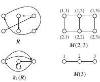
Refer to caption — Figure 1: A routing graph $R$ on $M(2,3)$ and $\bar{\pi}_{1}(R)$ on $M(3)$ .

An embedding $\langle\phi,\rho\rangle$ of a graph $G$ into a graph $H$ is a pair of mappings consisting of a one-to-one mapping $\phi:V(G)\rightarrow V(H)$ and a routing $\rho$ of an arbitrary orientation of the graph with the node set $V(H)$ and edge set $\{(\phi(u),\phi(v))\mid(u,v)\in E(G)\}$ . The dilation and edge-congestion of the embedding $\langle\phi,\rho\rangle$ are defined as the dilation and edge-congestion of $\rho$ , respectively.

3 Edge-Separators with Bounded Expansion

The (recursive) node- and edge-separators are formally defined as follows: Let $1/2\leq\beta<1$ and $s(n)$ be a non-decreasing function. A graph $G$ has a $\beta$ -node(edge, resp.)-separator of size $s(n)$ if $|V(G)|=1$ , or if $G$ can be partitioned into two subgraphs with at most $\beta|V(G)|$ nodes ( $\lceil\beta|V(G)|\rceil$ nodes, resp.) and with no edges connecting the subgraphs by removing at most $s(|V(G)|)$ nodes (edges, resp.), and the subgraphs recursively have a $\beta$ -node(edge, resp.)-separator of size $s(n)$ . The process of partitioning $G$ into isolated nodes using the edge-separator repeatedly is often referred to as a decomposition tree. The decomposition tree $\mathcal{T}$ is a rooted tree having a set of subgraphs of $G$ as its node set $V(\mathcal{T})$ such that the root of $\mathcal{T}$ is $G$ , each non-leaf node $H\in V(\mathcal{T})$ has exactly two children obtained from $H$ by removing the edge-separator of $H$ , and that each leaf node of $\mathcal{T}$ consists of a single node of $G$ . We call $\mathcal{T}$ a $\beta$ -decomposition tree with expansion $x(n)$ if it can be constructed using a $\beta$ -edge-separator, and for each $H\in V(\mathcal{T})$ , at most $x(|V(H)|)$ edges (called external edges of $H$ in this paper) connect $V(H)$ and $V(G)\setminus V(H)$ (Fig. 2).

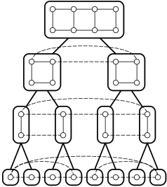
A decomposition tree with reasonably small expansion can be obtained from a node-separator as stated in the following lemma:

Lemma 1

Any graph $G$ with maximum node degree $\Delta$ and a $\beta$ -node-separator of size $Cn^{\alpha}$ ( $C>0$ , $0\leq\alpha<1$ , $1/2\leq\beta<1$ ) has a $\frac{\beta}{1-\epsilon}$ -decomposition tree with expansion $O(C\Delta n^{\alpha}/\epsilon)$ , where $0<\epsilon<1-\beta$ .

Proof 1

We present an algorithm constructing a desired decomposition tree $\mathcal{T}$ . We initially set $G$ as the root of $\mathcal{T}$ and construct $\mathcal{T}$ from the root toward leaves. Assume that we have constructed $\mathcal{T}$ up to depth (distance to the root) $i-1\geq 0$ . For a subgraph $H$ of $G$ at depth $i-1$ in $\mathcal{T}$ , we construct children $H_{1}$ and $H_{2}$ of $H$ as follows:

1.
We inductively assume the following:
1. (a)
  
  Each node of $\mathcal{T}$ up to depth $i-1$ has been constructed by partitioning a subgraph of $G$ using a $\beta$ -node-separator and distributing the node-separator between the partitioned graphs. Let $X_{i-1}$ be the set of nodes of $H$ contained in the node-separator used for any ancestor of $H$ in $\mathcal{T}$ .
2. (b)
  
  All the external edges of $H$ are incident to nodes in $X_{i-1}$ .
3. (c)
  
  The graph $H^{\prime}$ obtained from $H$ by removing $X_{i-1}$ has a $\beta$ -node-separator $S_{i}\subseteq V(H^{\prime})$ of size $Cn^{\alpha}$ .
It should be noted that $X_{0}=\emptyset$ , and therefore, these assumptions hold if $H=G$ .
2.

If $C|V(H^{\prime})|^{\alpha}\leq\epsilon|V(H^{\prime})|$ , then we partition $H^{\prime}$ into subgraphs $H^{\prime}_{1}$ and $H^{\prime}_{2}$ using the node-separator $S_{i}$ with $|S_{i}|\leq C|V(H^{\prime})|^{\alpha}$ . It follows that $|V(H^{\prime}_{1})|+|V(H^{\prime}_{2})|=|V(H^{\prime})|-|S_{i}|\geq(1-\epsilon)|V(H^{\prime})|\geq\frac{1-\epsilon}{\beta}|V(H^{\prime}_{1})|.$ Assume without loss of generality that $|V(H^{\prime}_{1})|\geq|V(H^{\prime}_{2})|$ . Then, there exists $1/2\leq\beta^{\prime}\leq\frac{\beta}{1-\epsilon}$ with $|V(H^{\prime}_{1})|=\beta^{\prime}(|V(H^{\prime}_{1})|+|V(H^{\prime}_{2})|)$ .
3.

If $C|V(H^{\prime})|^{\alpha}>\epsilon|V(H^{\prime})|$ , then reset $S_{i}:=V(H^{\prime})$ , and arbitrarily choose $1/2\leq\beta^{\prime}\leq\frac{\beta}{1-\epsilon}$ .
4.

Partition $X_{i-1}\cup S_{i}$ into two disjoint sets $Y_{1}$ and $Y_{2}$ such that $|Y_{1}|=\lceil\beta^{\prime}(|X_{i-1}|+|S_{i}|)\rceil$ and $|Y_{2}|=\lfloor(1-\beta^{\prime})(|X_{i-1}|+|S_{i}|)\rfloor$ .
5.

Let $H_{j}$ be the subgraph of $H$ induced by $V(H^{\prime}_{j})\cup Y_{j}$ for $j=1,2$ . We illustrate the construction in Fig. 3.

We first observe that $H_{1}$ and $H_{2}$ satisfy the inductive assumptions of the algorithm. For $j\in\{1,2\}$ , by inductive assumption, $Y_{j}$ is the set of nodes of $H_{j}$ contained in the node-separator used for an ancestor of $H_{j}$ . As shown in Fig. 3, all the external edges of $H_{j}$ are incident to nodes of $Y_{j}$ . Moreover, the subgraph of $H_{j}$ obtained by removing $Y_{j}$ is $H^{\prime}_{j}$ , which is the subgraph of $H^{\prime}$ partitioned by the node-separator $S_{i}$ of $H^{\prime}$ . Therefore, $H^{\prime}_{j}$ has a $\beta$ -node-separator of size $Cn^{\alpha}$ .

We then estimate the numbers of nodes of $H_{1}$ and $H_{2}$ . By definition, it follows that

	$\displaystyle\begin{split}\|V(H_{1})\|&=\|V(H^{\prime}_{1})\|+\|Y_{1}\|=\beta^{\prime}(\|V(H^{\prime}_{1})\|+\|V(H^{\prime}_{2})\|)+\lceil\beta^{\prime}(\|X_{i-1}\|+\|S_{i}\|)\rceil\\ &=\lceil\beta^{\prime}\|V(H)\|\rceil,\ \text{and}\end{split}$			(1)
	$\displaystyle\begin{split}\|V(H_{2})\|&=\|V(H^{\prime}_{2})\|+\|Y_{2}\|=(1-\beta^{\prime})(\|V(H^{\prime}_{1})\|+\|V(H^{\prime}_{2})\|)+\lfloor(1-\beta^{\prime})(\|X_{i-1}\|+\|S_{i}\|)\rfloor\\ &=\lfloor(1-\beta^{\prime})\|V(H)\|\rfloor\leq\beta^{\prime}\|V(H)\|.\end{split}$			(2)

These imply that the algorithm constructs $\mathcal{T}$ as a $\beta^{\prime}$ -decomposition tree of $G$ .

We finally prove that for $j=1,2$ , $H_{j}$ has $O(C\Delta|V(H_{j})|^{\alpha}/\epsilon)$ external edges, implying expansion $O(C\Delta n^{\alpha}/\epsilon)$ of $\mathcal{T}$ . We prove this only for $H_{1}$ because the proof for $H_{2}$ is obtained with a similar argument. Because all the external edges of $H_{1}$ are incident to $Y_{1}$ , it suffices to show that $|Y_{1}|=O(C|V(H_{1})|^{\alpha}/\epsilon)$ . When we construct children of $H_{1}$ using the algorithm, $X_{i}$ is set to $Y_{1}$ . Let $n_{i}:=|V(H_{1})|$ and $n_{j}$ ( $0\leq j<i$ ) be the number of nodes of the ancestor of $H_{1}$ at depth $j$ in $\mathcal{T}$ . Moreover, let $\beta_{j}$ ( $1\leq j\leq i$ ) be $\beta^{\prime}$ or $1-\beta^{\prime}$ defined in Step 2 or 3 in partitioning the ancestor at depth $j-1$ . This implies that $n_{j}=\lceil\beta_{j}n_{j-1}\rceil$ as in (1) or $n_{j}=\lfloor\beta_{j}n_{j-1}\rfloor$ as in (2). Therefore,

	$\displaystyle n_{j}$	$\displaystyle\leq\lceil\beta_{j}n_{j-1}\rceil\leq\beta_{j}n_{j-1}+1\leq n_{0}\prod_{h=1}^{j}\beta_{h}+\sum_{\ell=1}^{j}\prod_{h=\ell+1}^{j}\beta_{h}=n_{0}\prod_{h=1}^{j}\beta_{h}+O(1),\ \text{and}$		(3)
	$\displaystyle n_{j}$	$\displaystyle\geq\lfloor\beta_{j}n_{j-1}\rfloor\geq\beta_{j}n_{j-1}-1\geq n_{0}\prod_{h=1}^{j}\beta_{h}-\sum_{\ell=1}^{j}\prod_{h=\ell+1}^{j}\beta_{h}=n_{0}\prod_{h=1}^{j}\beta_{h}-O(1).$		(4)

Here, we have used the fact that $\sum_{\ell=1}^{j}\prod_{h=\ell+1}^{j}\beta_{h}\leq\sum_{\ell=1}^{j}(\frac{\beta}{1-\epsilon})^{j-\ell}=O(1)$ . By the definition of $Y_{1}$ , we have the following recurrence of $|X_{i}|$ :

|X_{i}|=|Y_{1}|=\lceil\beta_{i}(|X_{i-1}|+|S_{i}|)\rceil\leq\beta_{i}(|X_{i-1}|+|S_{i}|)+1\leq\sum_{j=1}^{i}|S_{j}|\prod_{h=j}^{i}\beta_{h}+\sum_{j=1}^{i}\prod_{h=j+1}^{i}\beta_{h}.

The number $|S_{j}|$ is less than $Cn_{j-1}^{\alpha}/\epsilon$ because $|S_{j}|\leq C|V(H^{\prime})|^{\alpha}\leq Cn_{j-1}^{\alpha}<Cn_{j-1}^{\alpha}/\epsilon$ if $S_{j}$ is defined in Step 2, and $|S_{j}|=|V(H^{\prime})|<C|V(H^{\prime})|^{\alpha}/\epsilon\leq Cn_{j-1}^{\alpha}/\epsilon$ if $S_{j}$ is defined in Step 3. Moreover, $\sum_{j=1}^{i}\prod_{h=j+1}^{i}\beta_{h}=O(1)$ as estimated for (3) and (4). Therefore,

\begin{split}|Y_{1}|&<\sum_{j=1}^{i}\frac{Cn_{j-1}^{\alpha}}{\epsilon}\prod_{h=j}^{i}\beta_{h}+O(1)\leq\sum_{j=1}^{i}\frac{C}{\epsilon}\left(n_{0}\prod_{h=1}^{j-1}\beta_{h}+O(1)\right)^{\alpha}\prod_{h=j}^{i}\beta_{h}+O(1)\quad\text{[by (\ref{eq:nj_upperbound})]}\\ &=O\left(\frac{Cn_{0}^{\alpha}}{\epsilon}\sum_{j=1}^{i}\prod_{h=1}^{j-1}\beta_{h}^{\alpha}\cdot\prod_{h=j}^{i}\beta_{h}\right)=O\left(\frac{Cn_{0}^{\alpha}}{\epsilon}\prod_{h=1}^{i}\beta_{h}^{\alpha}\cdot\sum_{j=1}^{i}\prod_{h=j}^{i}\beta_{h}^{1-\alpha}\right)\\ &=O\left(\frac{C}{\epsilon}\left(n_{0}\prod_{h=1}^{i}\beta_{h}\right)^{\alpha}\cdot\sum_{j=1}^{i}\left(\frac{\beta}{1-\epsilon}\right)^{(1-\alpha)(i-j+1)}\right)\\ &=O\left(\frac{C}{\epsilon}(n_{i}+O(1))^{\alpha}\cdot O(1)\right)\quad\text{[by (\ref{eq:nj_lowerbound})]}\\ &=O\left(\frac{Cn_{i}^{\alpha}}{\epsilon}\right).\\ \end{split}

Therefore, $\mathcal{T}$ is a desired decomposition tree. $\Box$

4 Embedding Algorithm

In this section, we first prove Theorem 1 by estimating the edge-congestion of the previously known permutation routing algorithm on multidimensional grids presented in [21]. We then provide an embedding algorithm based on edge-separators with bounded expansion as well as the permutation routing algorithm. Combining this algorithm with Lemma 1, we prove Theorem 2.

4.1 Permutation Routing and Embedding

Any permutation routing can be used to construct a graph embedding as follows:

Lemma 2

If any $1$ - $1$ routing graph on a host graph $H$ can be routed with an edge-congestion at most $c$ , then any graph with maximum node degree $\Delta$ can be embedded into $H$ with an edge-congestion at most $c\lceil\Delta/2\rceil$ .

Proof 2

Let $G$ be a graph with maximum node degree $\Delta$ to be embedded into $H$ . We arbitrarily choose a one-to-one mapping $\phi:V(G)\rightarrow V(H)$ . Let $G^{\prime}$ be the graph with node set $\phi(V(G))$ and edge set $\{(\phi(u),\phi(v))\mid(u,v)\in E(G)\}$ . Because $G^{\prime}$ is an undirected graph with maximum node degree $\Delta$ , there is an orientation $R$ of $G^{\prime}$ whose maximum indegree and outdegree are both at most $\lceil\Delta/2\rceil$ . Such an orientation can be obtained by adding dummy edges joining nodes with odd degree so that the resulting graph has an Euler circuit, and by orienting edges along with the Euler circuit. It suffices to prove that $R$ as a routing graph on $H$ can be routed with an edge-congestion at most $c\lceil\Delta/2\rceil$ .

We decompose $R$ into at most $\lceil\Delta/2\rceil$ edge-disjoint $1$ - $1$ routing graphs each of which has nodes $V(R)$ and edges with the same color in an edge-coloring of $R$ such that no two edges with the same sources or with the same targets have the same color. Such coloring can be obtained by edge-coloring the bipartite graph consisting of the source and target sets of $R$ , i.e., two copies $V^{+}$ and $V^{-}$ of $V(R)$ , and edges joining $u\in V^{+}$ and $v\in V^{-}$ for all $(u,v)\in E(R)$ . It should be noted that the resulting bipartite graph has node-degree at most $\lceil\Delta/2\rceil$ , and hence, $\lceil\Delta/2\rceil$ colors are enough for the coloring. Therefore, $R$ can be routed on $H$ with an edge-congestion at most $c\lceil\Delta/2\rceil$ if each of the $1$ - $1$ routing graphs can be routed with an edge-congestion at most $c$ . $\Box$

The algorithm of [21] routes a $1$ - $1$ routing graph $R$ on $M:=M(\ell_{i})_{i\in[d]}$ as follows:

1.

Color edges of $R$ using at most $\ell_{1}$ colors so that when we identify edges in $R$ with corresponding edges in $\bar{\pi}_{1}(R)$ , no two edges with the same sources or with the same targets in $\bar{\pi}_{1}(R)$ have the same color. This coloring can be obtained as done in the proof of Lemma 2. It should be noted that $\bar{\pi}_{1}(R)$ is a $\ell_{1}$ - $\ell_{1}$ routing graph with node set $\bar{\pi}_{1}(V(M))$ .
2.

Decompose $R$ into edge-disjoint subgraphs $R_{1},\ldots,R_{\ell_{1}}$ each of which has nodes $V(R)$ and edges with the same color.
3.

For each $i\in[\ell_{1}]$ , $\bar{\pi}_{1}(R_{i})$ is a $1$ - $1$ routing graph with node set $\bar{\pi}_{1}(V(M))$ . Therefore, we can recursively find a routing $\rho_{i}$ of $\bar{\pi}_{1}(R_{i})$ on the $(d-1)$ -dimensional subgrid $M_{i}$ induced by the nodes $\{v\in V(M)\mid\pi_{1}(v)=i\}$ . If $d=2$ , i.e., if $M_{i}$ is a path, then $\rho_{i}$ simply routes each routing request of $\bar{\pi}_{1}(R_{i})$ on the path connecting its source and target in $M_{i}$ .
4.

We route each $(s,t)\in E(R_{i})$ on the edge set consisting of dimension- $1$ edges connecting $s$ to $M_{i}$ , $\rho_{i}(\bar{\pi}_{1}(s),\bar{\pi}_{1}(t))$ , and dimension- $1$ edges connecting $t$ to $M_{i}$ .

We can easily observe that in this algorithm, any dimension- $i$ edge of $M$ is contained in at most $2\ell_{i}$ images of $\rho$ . Moreover, each image of $\rho$ contains at most $2\ell_{i}$ dimension- $i$ edges. I.e., $\rho$ has an edge-congestion of $2\cdot\max_{i\in[d]}\{\ell_{i}\}$ and a dilation of $2\sum_{i=1}^{d}\ell_{i}$ . This property and Lemma 2 prove Theorem 1. With our aim of using this permutation routing algorithm to prove Theorem 2, we generalize this property as the following lemma:

Lemma 3

Let $R$ be a routing graph on $M:=M(\ell_{i})_{i\in[d]}$ with $d\geq 2$ and $\ell_{h}:=\max_{i\in[d]}\{\ell_{i}\}$ . If $\bar{\pi}_{h}(R)$ is a $p$ - $q$ routing graph with node set $\bar{\pi}_{h}(V(M))$ , then $R$ can be routed on $M$ with a dilation at most $2\sum_{i=1}^{d}\ell_{i}$ and an edge-congestion at most $2\cdot\max\{p,q\}$ .

Proof 3

Assume without loss of generality that $h=1$ and $\ell_{1}\geq\cdots\geq\ell_{d}$ . We prove the lemma by induction on $d$ . If $d=2$ , then $R$ has at most $\ell_{2}\cdot\max\{p,q\}$ edges. We decompose $R$ into $\ell_{1}$ edge-disjoint subgraphs $R_{1},\ldots,R_{\ell_{1}}$ so that $\bigcup_{i=1}^{\ell_{1}}E(R_{i})=E(R)$ and $|E(R_{i})|\leq\lceil\ell_{2}\cdot\max\{p,q\}/\ell_{1}\rceil\leq\max\{p,q\}$ for $i\in[\ell_{1}]$ . For each $i\in[\ell_{1}]$ , $\bar{\pi}_{1}(R_{i})$ can be routed on the $1$ -dimensional grid $M_{i}$ induced by the nodes $\{v\in V(M)\mid\pi_{1}(v)=i\}$ with a dilation at most $\ell_{2}$ and an edge-congestion at most $\max\{p,q\}$ . The routing of $R$ is completed by adding the dimension- $1$ edges connecting $s$ to $M_{i}$ and $t$ to $M_{i}$ for each $(s,t)\in E(R_{i})$ . Any dimension- $1$ edge has a congestion at most $p+q$ . Moreover, at most $2\ell_{1}$ dimension- $1$ edges are added to each image of the routing. Therefore, we have the lemma for $d=2$ .

If $d\geq 3$ , then we color edges of $R$ using at most $\ell_{2}\cdot\max\{p,q\}$ colors so that when we identify edges in $R$ with corresponding edges in $\bar{\pi}_{2}(\bar{\pi}_{1}(R))$ , no two edges with the same sources or with the same targets in $\bar{\pi}_{2}(\bar{\pi}_{1}(R))$ have the same color. Such coloring exists because $\bar{\pi}_{2}(\bar{\pi}_{1}(R))$ is a $\ell_{2}p$ - $\ell_{2}q$ routing graph with node set $\bar{\pi}_{2}(\bar{\pi}_{1}(V(M)))$ . Then, we decompose $R$ into $\ell_{1}$ edge-disjoint subgraphs $R_{1},\ldots,R_{\ell_{1}}$ that have edge sets with disjoint sets of $\lceil\ell_{2}\cdot\max\{p,q\}/\ell_{1}\rceil\leq\max\{p,q\}$ colors. This implies that $\bar{\pi}_{2}(\bar{\pi}_{1}(R_{i}))$ is a $\max\{p,q\}$ - $\max\{p,q\}$ routing graph with node set $\bar{\pi}_{2}(\bar{\pi}_{1}(V(M)))$ for $i\in[\ell_{1}]$ . By induction hypothesis, $\bar{\pi}_{1}(R_{i})$ can be routed on the $(d-1)$ -dimensional subgrid induced by the nodes $\{v\in V(M)\mid\pi_{1}(v)=i\}$ with a dilation at most $2\sum_{i=2}^{d}\ell_{i}$ and an edge-congestion at most $2\cdot\max\{p,q\}$ . The routing of $R$ is completed by adding dimension- $1$ edges as done in the case of $d=2$ , so that any dimension- $1$ edge has congestion at most $p+q$ , and at most $2\ell_{1}$ dimension- $1$ edges are added to each image of the routing. Thus, we have routed $R$ with a dilation at most $2\sum_{i=1}^{d}\ell_{i}$ and an edge-congestion at most $2\cdot\max\{p,q\}$ . $\Box$

If we do not have the assumption $\ell_{h}=\max_{i\in[d]}\{\ell_{i}\}$ in Lemma 3, then we can estimate $\lceil\ell_{2}\cdot\max\{p,q\}/\ell_{1}\rceil\leq\lceil\mu\cdot\max\{p,q\}\rceil$ in its proof, where $\mu$ is the aspect ratio of $M$ . This means that $|E(R_{i})|\leq\lceil\mu\cdot\max\{p,q\}\rceil$ for $d=2$ , and that $\bar{\pi}_{2}(\bar{\pi}_{1}(R_{i}))$ is a $\lceil\mu\cdot\max\{p,q\}\rceil$ - $\lceil\mu\cdot\max\{p,q\}\rceil$ routing graph on $\bar{\pi}_{2}(\bar{\pi}_{1}(M))$ for $d\geq 3$ . Therefore, initially assuming without loss of generality that $\ell_{1}=\ell_{h}$ and $\ell_{2}\geq\cdots\geq\ell_{d}$ in the proof, we have the following lemma:

Lemma 4

Let $R$ be a routing graph on $M:=M(\ell_{i})_{i\in[d]}$ with $d\geq 2$ and aspect ratio $\mu$ . If $\bar{\pi}_{h}(R)$ is a $p$ - $q$ routing graph with node set $\bar{\pi}_{h}(V(M))$ for some $h\in[d]$ , then $R$ can be routed on $M$ with a dilation at most $2\sum_{i=1}^{d}\ell_{i}$ and an edge-congestion at most $2\lceil\mu\cdot\max\{p,q\}\rceil$ .

4.2 Separator-Based Embedding

The following is our core theorem:

Theorem 3

Suppose that $G$ is a graph with $N$ nodes, maximum node degree $\Delta$ , and with a $\beta$ -decomposition tree of expansion $Cn^{\alpha}$ ( $C>0$ , $0\leq\alpha<1$ , $1/2\leq\beta<1$ ), and that $M$ is a grid with a dimension $d\geq 2$ , at least $N$ nodes, and with constant aspect ratio. Then, $G$ can be embedded into $M$ with a dilation of $O(dN^{1/d})$ , and with an edge-congestion of $O(dC+d^{2}\Delta)$ if $d>2/(1-\alpha)$ , $O(C/(1-\alpha-\frac{1}{d})+d^{2}\Delta)$ if $1/(1-\alpha)<d\leq 2/(1-\alpha)$ , and $O(C(N^{\alpha-1+\frac{1}{d}}+\log N)+d^{2}\Delta)$ if $d\leq 1/(1-\alpha)$ ,

In fact, we can obtain Theorem 2 by combining Theorem 3 with Lemma 1. If $G$ is a graph with $N$ nodes, maximum node degree $\Delta$ , and with a $\beta$ -node-separator of size $O(n^{\alpha})$ , then by Lemma 1, $G$ has a $\frac{\beta}{1-\epsilon}$ -decomposition tree with expansion $O(\Delta n^{\alpha}/\epsilon)=O(\Delta n^{\alpha})$ for any $0<\epsilon<1-\beta$ . By Theorem 3, therefore, $G$ can be embedded into $M$ with a dilation of $O(dN^{\frac{1}{d}})$ , and with an edge-congestion of $O(\Delta\cdot\max\{d,1/(1-\alpha-\frac{1}{d})\}+d^{2}\Delta)=O(\Delta)$ if $d>1/(1-\alpha)$ is fixed, $O(\Delta(N^{\alpha-1+\frac{1}{d}}+\log N)+d^{2}\Delta)=O(\Delta\log N)$ if $d=1/(1-\alpha)$ , and $O(\Delta(N^{\alpha-1+\frac{1}{d}}+\log N)+d^{2}\Delta)=O(\Delta N^{\alpha-1+\frac{1}{d}})$ if $d<1/(1-\alpha)$ .

We prove Theorem 3 by constructing a desired embedding algorithm, called SBE. We first outline ideas and analysis of SBE, then specify the definition of SBE, and finally prove the correctness and the edge-congestion.

Proof Sketch

We describe a proof sketch for the case $1/(1-\alpha)<d\leq 2/(1-\alpha)$ since essential part of idea appears in this case. Basically, we partition $G$ according to its decomposition tree, recursively embed the partitioned subgraphs of $G$ into partitioned subgrids of the host grid $M:=M(\ell_{i})_{i\in[d]}$ , and route cut edges, i.e., edges removed in partitioning $G$ . In order to avoid an edge of $M$ being used in too many recursive steps, we route the cut edges on one of edge-disjoint subgraphs of $M$ , called channels. The channel associated with a positive integer $w$ roughly equal to $\frac{1}{2}(1-\alpha-\frac{1}{d})\log_{2}N$ is a grid-like graph homeomorphic to $M^{\prime}:=M(\frac{\ell_{1}}{2^{w}},\frac{\ell_{2}}{2^{w}},\ell_{3},\ldots,\ell_{d})$ and induced by the nodes $v\in V(M)$ with $\pi_{i}(v)\equiv 2^{w-1}\pmod{2^{w}}$ for each $i=1,2$ . We can find the channel in $M$ as a non-empty subgraph if $d\leq 2/(1-\alpha)$ . When we embed an $n$ -node subgraph $H$ of $G$ appeared in the decomposition tree, we partially route the external edges of each child of $H$ to the channel associated with $w\simeq\frac{1}{2}(1-\alpha-\frac{1}{d})\log_{2}n$ and route the cut edges of $H$ by connecting the two sets of the external edges of children of $H$ on this channel. We here say “partially” in two meanings: One meaning is that external edges are viewed as half-edges just leaving a child of $H$ and are routed halfway. The other is that an external edge leaving a node in the decomposition tree is also an external edge of some descendants and is routed step by step among recursive steps. I.e., a cut edge is routed by connecting two partially routed external edges of the children, which are recursively routed using partially routed external edges of grandchildren, and so on. Consequently, cut edges of $H$ are routed through channels associated with integers up to $\frac{1}{2}(1-\alpha-\frac{1}{d})\log_{2}n$ in recursive steps from base embeddings to the embedding of $H$ .

The section of $M^{\prime}$ across a dimension $i$ is a $(d-1)$ -dimensional grid with node set $\bar{\pi}_{i}(V(M^{\prime}))$ . If $M^{\prime}$ is associated with $w=\frac{1}{2}(1-\alpha-\frac{1}{d})\log_{2}n$ , then the minimum size $S$ of the section is $\min_{i}|\bar{\pi}_{i}(V(M^{\prime}))|=\Omega(n^{(d-1)/d}/2^{2w})=\Omega(n^{\alpha})$ . Since $H$ and children of $H$ have at most $Cn^{\alpha}$ external edges, we route the external edges (or half-edges) of each child to the channel so that at most $D:=Cn^{\alpha}/S=O(C)$ halfway points $v$ have the same $\bar{\pi}_{i}(v)$ , where $i$ minimizes $|\bar{\pi}_{i}(V(M^{\prime}))|$ . We can inductively observe that this routing can be done with an edge-congestion $O(D)$ using Lemma 3. The integer $w$ decreases after $P=O(1/(1-\alpha-\frac{1}{d}))$ recursive steps proceed because a guest graph becomes roughly half in one recursive step. Therefore, the total edge-congestion incurred by entire recursive steps is at most $O(PD)=O(C/(1-\alpha-\frac{1}{d}))$ since channels associated with different $w$ ’s are edge-disjoint. We stop the recursive procedure at the point $\min\{\ell_{i}\}=\Theta(d)$ , by which we can obtain a base embedding with an edge-congestion $B=O(d\Delta)$ using Lemmas 2–4. Because an edge of $M$ can possibly be contained in $O(d)$ base embeddings, the total edge-congestion is at most $O(PD+dB)=O(C/(1-\alpha-\frac{1}{d})+d^{2}\Delta)$ .

The reason of the limit $\min\{\ell_{i}\}=\Theta(d)$ of recursive procedure is as follows: We cannot always partition the host grid with a “flat” section due to the difference between the number of nodes of a partitioned guest graph and multiples of the size of the section. In our algorithm, therefore, we partition a host grid into two subgrids that may share a $(d-1)$ -dimensional grid as “ragged” sections. Such a $(d-1)$ -dimensional grid might be used as channels in two partitioned grids during $O(d)$ recursive steps in the worst case, which would yield a $2^{O(d)}$ factor in the edge-congestion. To avoid this, we actually remove any boundary of a host grid from a channel, so that two partitioned grids have disjoint channels. However, we might have an exponential factor again if we would continue the recursive procedure until $\min\{\ell_{i}\}$ is much smaller than $d$ . For instance, if $\min\{\ell_{i}\}=O(1)$ , then removal of the boundary for each dimension would shrink the channel exponentially, implying $S=n^{\alpha}/2^{O(d)}$ and hence $D=O(C2^{O(d)})$ .

Definition of SBE

Suppose that $G_{0}$ and $M_{0}$ are a guest graph and a host grid, respectively, satisfying the conditions of Theorem 3. Let $\mathcal{T}$ be a $\beta$ -decomposition tree for $G_{0}$ with expansion $Cn^{\alpha}$ . We set $\mu$ to the larger number of the aspect ratio of $M_{0}$ and

\frac{1}{1-\beta}\left(\frac{1}{7\beta}+e\beta\right)+\frac{5}{4}>4,

where $e$ is base of the natural logarithm. We assume that any proper subgrid of $M_{0}$ has less than $N$ nodes.

We use the following notations to define SBE formally: Let $V^{w}:=\{v\in V(M_{0})\mid\pi_{i}(v)\equiv 2^{w-1}\pmod{2^{w}}\text{ for each $i=1,2$}\}$ for an integer $w\geq 1$ , and let $V^{0}:=V(M_{0})$ . For a $d$ -dimensional subgrid $M$ of $M_{0}$ , let $W_{M}^{w}:=\{v\in V^{w}\cap V(M)\mid\deg_{M}(v)=2d\}$ , where $\deg_{M}(\cdot)$ is the node degree in $M$ . The channel of $W_{M}^{w}$ is the subgraph of $M$ homeomorphic to a $d$ -dimensional grid having $W_{M}^{w}$ as grid points. Specifically, this graph is induced by the node set $W_{M}^{w}\cup\{s\in V(M)\mid\exists i\in\{1,2\}\ \exists\{u,v\}\subseteq W_{M}^{w}\ \pi_{i}(u)<\pi_{i}(s)<\pi_{i}(v)=\pi_{i}(u)+2^{w},\ \bar{\pi}_{i}(u)=\bar{\pi}_{i}(s)=\bar{\pi}_{i}(v)\}$ . Two channels in $M(8,8,4)$ are illustrated in Fig. 4. It should be noted that for any $w>w^{\prime}\geq 1$ , $W_{M}^{w}\cap W_{M}^{w^{\prime}}=\emptyset$ and channels of $W_{M}^{w}$ and $W_{M}^{w^{\prime}}$ are edge-disjoint. The direction of $W_{M}^{w}$ is a dimension $i\in[d]$ minimizing $S_{M}^{i,w}:=|\bar{\pi}_{i}(W_{M}^{w})|$ . In other words, the direction is a dimension of the longest side length of a grid having grid points $W_{M}^{w}$ . In Fig. 4, the channel for $w=1$ has direction $1$ or $2$ because $S_{M}^{1,1}=S_{M}^{2,1}=6$ and $S_{M}^{3,1}=9$ . A mapping $\psi:X\rightarrow W_{M}^{w}$ is said to be uniform across dimension $i$ if $\psi(X)$ are uniformly distributed on $\bar{\pi}_{i}(W_{M}^{w})$ , i.e., $\lambda_{i}(\psi):=\max_{v\in\bar{\pi}_{i}(W_{M}^{w})}|\{s\in X\mid\bar{\pi}_{i}(\psi(s))=v\}|=\lceil|X|/S_{M}^{i,w}\rceil$ . In Fig. 4, for example, if $\psi:[4]\rightarrow W_{M}^{1}$ maps $1,2,3,4$ to $(3,3,2),(3,5,2),(5,3,3),(5,5,3)$ , respectively, then $\psi$ is uniform across dimensions both $1$ and $3$ but not dimension $2$ because $\lambda_{1}(\psi)=1=\lceil|[4]|/S_{M}^{1,1}\rceil=\lceil 4/6\rceil$ , $\lambda_{2}(\psi)=2>\lceil|[4]|/S_{M}^{2,1}\rceil=\lceil 4/6\rceil$ , and $\lambda_{3}(\psi)=1=\lceil|[4]|/S_{M}^{3,1}\rceil=\lceil 4/9\rceil$ . We note here that for any two dimensions $i$ and $j$ , we can construct $\psi$ uniform across dimensions both $i$ and $j$ by uniformly distributing $\psi(X)$ among nodes on a $(d-1)$ -dimensional diagonal hyperplane between dimensions $i$ and $j$ in $W_{M}^{w}$ .

Step 0—Input and Output

The formal input and output of SBE is as follows:

Algorithm SBE( $G$ , $X$ , $M$ , $U$ )

Input

1.

An $n$ -node subgraph $G$ of $G_{0}$ contained in $V(\mathcal{T})$ .
2.

A multiset $X$ of nodes of $G$ incident to distinct external edges of $G$ , i.e., a node appears in $X$ as many times as the number of the external edges incident to the node.
3.

A subgrid $M=M(\ell_{i})_{i\in[d]}$ of $M_{0}$ with aspect ratio at most $\mu$ , together with a set $U\subseteq V(M)$ such that $U\supseteq\{v\in V(M)\mid\deg_{M}(v)=2d\}$ and $|U|=n$ . Suppose that $h$ is a dimension such that $\ell_{h}=\max_{i\in[d]}\{\ell_{i}\}$ .

Output

1.

An embedding $\langle\phi,\rho\rangle$ of $G$ into $M$ such that $\phi(V(G))=U$ .
2.

A mapping $\psi:X\rightarrow W_{M}^{w}$ uniform across the direction $k$ of $W_{M}^{w}$ , where $w\geq 0$ is an integer defined in Step 1.
3.

A routing $\sigma$ of the routing graph with node set $\phi(X)\cup\psi(X)$ and edge set $\{(\phi(u),\psi(u))\mid u\in X\}$ .

Initially, we arbitrarily choose $U$ as desired and perform SBE( $G_{0}$ , $\emptyset$ , $M_{0}$ , $U$ ).

Step 1—Channel Configuration

This step sets an integer $w$ , by which we configure the channel of $W_{M}^{w}$ to route $\rho$ and $\sigma$ . We define $w:=\max\{\lfloor\frac{1}{2}((1-\tilde{\alpha}-\frac{1}{d})\log_{2}n-\log_{2}\frac{\mu}{1-\beta})\rfloor,0\}$ , where $\tilde{\alpha}:=\max\{1-\frac{2}{d},\alpha\}$ . In other words, $w=\max\{\lfloor\frac{1}{2}(\frac{1}{d}\log_{2}n-\log_{2}\frac{\mu}{1-\beta})\rfloor,0\}$ if $d>2/(1-\alpha)$ , $w=\max\{\lfloor\frac{1}{2}((1-\alpha-\frac{1}{d})\log_{2}n-\log_{2}\frac{\mu}{1-\beta})\rfloor,0\}$ if $1/(1-\alpha)<d\leq 2/(1-\alpha)$ , and $w=0$ if $d\leq 1/(1-\alpha)$ .

Step 2—Base Embedding

If $\ell_{h}\leq 2\mu d$ , then SBE does not call itself recursively any longer and constructs a base embedding as follows:

1.

If $X=\emptyset$ , then let $\phi:V(G)\rightarrow U$ be an arbitrary one-to-one mapping. Otherwise, let $Y$ be the set (not a multiset) of nodes incident to external edges of $G$ . We construct a one-to-one mapping $\phi:V(G)\rightarrow U$ so that degrees of nodes in $Y$ are uniformly distributed on $\bar{\pi}_{k}(U)$ . Specifically, for any $v\in\bar{\pi}_{k}(U)$ , the sum of degrees of nodes $s\in Y$ with $\bar{\pi}_{k}(\phi(s))=v$ is at most $e|X|/|\bar{\pi}_{k}(U)|+\Delta$ . We prove later in Lemma 5 that $\phi$ can be constructed as desired. This construction implies that if $R$ is the routing graph to be routed by $\sigma$ , then $\bar{\pi}_{k}(R)$ has maximum outdegree at most $e|X|/|\bar{\pi}_{k}(U)|+\Delta\leq e|X|/S_{M}^{k,w}+\Delta$ .
2.

Construct a mapping $\psi:X\rightarrow W_{M}^{w}$ so that $\psi$ is uniform across dimension $k$ , implying that $\bar{\pi}_{k}(R)$ has maximum indegree at most $\lceil|X|/S_{M}^{k,w}\rceil$ .
3.

Apply Lemmas 2 and 3 on $M$ to obtain $\rho$ .
4.

If $X\neq\emptyset$ , then apply Lemma 4 on $M$ to obtain $\sigma$ .
5.

Return.

Step 3—Partition

Suppose $\ell_{h}>2\mu d$ . Let $G_{1}$ and $G_{2}$ be children of $G$ in $\mathcal{T}$ and have $n_{1}$ and $n_{2}$ nodes, respectively. Now $M$ is partitioned into two subgrids $M_{1}:=M(\ell_{1},\ldots,\ell_{h-1},m_{1},\ell_{h+1},\linebreak\ldots,\ell_{d})$ and $M_{2}:=M(\ell_{1},\ldots,\ell_{h-1},m_{2},\ell_{h+1},\ldots,\ell_{d})$ , together with node sets $U_{1}\subseteq V(M_{1})$ and $U_{2}\subseteq V(M_{2})$ such that $m_{1}+m_{2}=\ell_{h}+1$ , $U_{1}\cup U_{2}=U$ , $U_{1}\cap U_{2}=\emptyset$ , and $|U_{j}|=n_{j}$ for $j=1,2$ (Fig 5). We here duplicate the $(d-1)$ -dimensional grid induced by $\{v\in V(M)\mid\pi_{h}(v)=m_{1}\}$ to be shared by $M_{1}$ and $M_{2}$ , so that $m_{1}+m_{2}$ equals not $\ell_{h}$ but $\ell_{h}+1$ . We do this because $M_{1}$ and $M_{2}$ must have enough numbers of nodes in $U$ onto which $V(G_{1})$ and $V(G_{2})$ can be mapped, respectively. In Fig 5, actually, however we partition $M$ so that $m_{1}+m_{2}=l_{h}$ , either $|V(M_{1})\cap U|<20$ or $|V(M_{2})\cap U|<30$ . We will prove later in Lemma 6 that the resulting subgrids have aspect ratio at most $\mu$ .

Step 4—Recursive Embedding

This step recursively embeds $G_{1}$ and $G_{2}$ into $M_{1}$ and $M_{2}$ , respectively. We also construct a routing $\tilde{\sigma}_{j}$ for $j=1,2$ , which draws the external edges of $G_{j}$ to $\tilde{\psi}_{j}(X_{j})$ . Here, $X_{j}$ is the multiset of nodes of $G_{j}$ incident to distinct external edges of $G_{j}$ , and $\tilde{\psi}_{j}:X_{j}\rightarrow W_{M_{j}}^{w}$ is a mapping uniform across dimension $k$ , i.e., the direction of $W_{M}^{w}$ . With this routing, in the subsequent step, we will make a routing graph with sources and targets in $\tilde{\psi}_{1}(X_{1})$ and $\tilde{\psi}_{2}(X_{2})$ , respectively, on the channel of $W_{M}^{w}$ to connect cut edges. Projecting this routing graph along dimension $k$ yields a $\lceil|X_{1}|/S_{M}^{k,w}\rceil$ - $\lceil|X_{2}|/S_{M}^{k,w}\rceil$ routing graph. Thus, the cut edges will be routed on the channel of $W_{M}^{w}$ with an edge-congestion of $2\cdot\max_{j=1,2}\lceil|X_{j}|/S_{M}^{k,w}\rceil$ using Lemma 3. In applying Lemma 3, we regard the underlying channel as the homeomorphic grid with grid points $W_{M}^{w}$ . A detailed analysis for this edge-congestion will later be provided in Lemmas 8-10. We aim to suppress the edge-congestion of $\tilde{\sigma}_{j}$ in a similar way. Therefore, we make $\tilde{\psi}_{j}$ uniform across not only dimension $k$ but also the direction $k_{j}$ of $W_{M_{j}}^{w_{j}}$ , where $w_{j}$ is $w$ computed for $n_{j}$ in the recursive procedure, since $\psi_{j}$ is made uniform across dimension $k_{j}$ in the recursive procedure (Fig 6). We need to treat two more matters in constructing $\tilde{\sigma}_{j}$ .

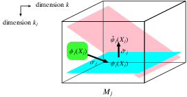
First, we need a channel (a grid-like graph) containing both $\psi_{j}(X_{j})\subseteq W_{M_{j}}^{w_{j}}$ and $\tilde{\psi}_{j}(X_{j})\subseteq W_{M_{j}}^{w}$ . Just taking union of two channels of $W_{M_{j}}^{w_{j}}$ and $W_{M_{j}}^{w}$ would not suffice because $W_{M_{j}}^{w_{j}}$ and $W_{M_{j}}^{w}$ are disjoint if $w_{j}\neq w$ . We define the channel for $w_{j}$ and $w$ as the graph homeomorphic to a $d$ -dimensional grid having $W_{M_{j}}^{w_{j},w}:=\{v\in V(M_{0})\mid\pi_{i}(v)\equiv 2^{w_{j}-1}\ \text{or}\ 2^{w-1}\pmod{2^{w}}\ \text{for $i=1,2$}\}\cap\{v\in V(M_{j})\mid\deg_{M_{j}}(v)=2d\}$ as grid points. It should be noted that if $w>w_{j}>0$ , then edges contained in the channel of $W_{M_{j}}^{w_{j},w}$ but in the channel of neither $W_{M_{j}}^{w_{j}}$ nor $W_{M_{j}}^{w}$ are uniquely determined by $w_{j}$ and $w$ and not contained any other channel in $M_{j}$ except the channel of $W_{M_{j}}^{0}$ .

The second matter is that the direction of $W_{M_{j}}^{w_{j},w}$ may differ from $k_{j}$ , across which $\psi_{j}$ and $\tilde{\psi}_{j}$ are uniform. This means that just applying Lemma 3 would not guarantee a desired edge-congestion. If we applied the algorithm of Lemma 3 on the channel of $W_{M_{j}}^{w_{j},w}$ , then the algorithm would be recursively called in the non-increasing order of side lengths of a grid having $W_{M_{j}}^{w_{j},w}$ as grid points. We here modify the order by replacing $W_{M_{j}}^{w_{j},w}$ with $W_{M_{j}}^{w_{j}}$ . The modified algorithm yields a desired edge-congestion as we will later prove in Lemma 8.

For each $j=1,2$ , specifically, SBE performs the following procedures:

1.

Call SBE( $G_{j}$ , $X_{j}$ , $M_{j}$ , $U_{j}$ ). Let $\phi_{j}$ , $\rho_{j}$ , $\psi_{j}$ , and $\sigma_{j}$ denote the output $\phi$ , $\rho$ , $\psi$ , and $\sigma$ of the recursive call, respectively.
2.

Construct a mapping $\tilde{\psi}_{j}:X_{j}\rightarrow W_{M_{j}}^{w}$ uniform across dimensions both $k$ and $k_{j}$ , where $k_{j}$ is the direction of $W_{M_{j}}^{w_{j}}$ , and $w_{j}:=\max\{\lfloor\frac{1}{2}((1-\tilde{\alpha}-\frac{1}{d})\log_{2}n_{j}-\log_{2}\frac{\mu}{1-\beta})\rfloor,0\}$ .
3.

Let $\tilde{\sigma}_{j}$ be a routing from $\psi_{j}(X_{j})$ to $\tilde{\psi}_{j}(X_{j})$ on the channel of $W_{M_{j}}^{w_{j},w}$ obtained by using the modified algorithm of Lemma 3 in which we recursively call the algorithm in the non-increasing order of side lengths of a grid having $W_{M_{j}}^{w_{j}}$ as grid points.

Step 5—Routing Cut and External Edges

This step constructs $\psi$ , then completes $\rho$ and $\sigma$ using $\tilde{\psi}_{j}$ and $\psi$ . The routings $\rho$ and $\sigma$ are obtained simply using Lemma 3 on the channel of $W_{M}^{w}$ since $\tilde{\psi}_{j}(X_{j})\subseteq W_{M_{j}}^{w}\subseteq W_{M}^{w}$ . The following are specific procedures of this step:

1.

Construct a mapping $\psi:X\rightarrow W_{M}^{w}$ uniform across dimension $k$ .
2.

By using Lemma 3, construct $\tilde{\sigma}$ for the routing graph on the channel of $W_{M}^{w}$ with node set $\tilde{\psi}_{1}(X_{1})\cup\tilde{\psi}_{2}(X_{2})$ and edge set $\{(\tilde{\psi}_{1}(s_{1}),\tilde{\psi}_{2}(s_{2}))\mid s_{1}\in X_{1}\setminus X,\ s_{2}\in X_{2}\setminus X,\ (s_{1},s_{2})\in E(G)\}\cup\bigcup_{j=1,2}\{(\tilde{\psi}_{j}(s),\psi(s))\mid s\in X_{j}\cap X\}$ (Fig 7). It should be noted that $(s_{1},s_{2})\in E(G)$ with $s_{1}\in X_{1}\setminus X$ and $s_{2}\in X_{2}\setminus X$ is a cut edge of $G$ , and $s\in X_{j}\cap X$ is a node incident to an external edge of $G$ .

Figure 7: Mapping $\psi$ and routing $\tilde{\sigma}$ constructed in Step 5. The left, center, and right planes represent the uniformness of $\tilde{\psi}_{1}(X_{1})$ , $\psi(X)$ , and $\tilde{\psi}_{2}(X_{2})$ , respectively.

Let $\rho$ map the cut edges of $G$ onto paths obtained by concatenating the images of $\sigma_{1}$ , $\tilde{\sigma}_{1}$ , $\tilde{\sigma}$ , $\tilde{\sigma}_{2}$ , and $\sigma_{2}$ . Specifically, for $(s_{1},s_{2})\in E(G)$ with $s_{1}\in X_{1}\setminus X$ and $s_{2}\in X_{2}\setminus X$ , let

\begin{split}\rho(\phi(s_{1}),\phi(s_{2})):=&\bigcup_{j=1,2}\left(\sigma_{j}(\phi(s_{j}),\psi_{j}(s_{j}))\cup\tilde{\sigma}_{j}(\psi_{j}(s_{j}),\tilde{\psi}_{j}(s_{j}))\right)\\ &\quad\cup\tilde{\sigma}(\tilde{\psi}_{1}(s_{1}),\tilde{\psi}_{2}(s_{2})).\end{split}

Let $\sigma$ map the external edges of $G$ onto paths obtained by concatenating the images of $\sigma_{j}$ , $\tilde{\sigma}_{j}$ , $\tilde{\sigma}$ . Specifically, for $s\in X_{j}\cap X$ ( $j=1,2$ ), let

\begin{split}\sigma(\phi(s),\psi(s)):=&\sigma_{j}(\phi(s),\psi_{j}(s))\cup\tilde{\sigma}_{j}(\psi_{j}(s),\tilde{\psi}_{j}(s))\cup\tilde{\sigma}(\tilde{\psi}_{j}(s),\psi(s)).\end{split}

Correctness

To prove that SBE yields an output satisfying the conditions specified in Step 0, we first prove in Lemma 5 below that we can construct $\phi$ as desired in Step 2 for the case $X\neq\emptyset$ . We then prove in Lemmas 6 and 7 below that $M_{j}$ defined in Step 3 has aspect ratio at most $\mu$ , and that $W_{M_{j}}^{w}$ is non-empty as well as $W_{M}^{w}$ . These facts guarantee that a valid input is given to a child procedure in Step 4, and that mappings $\tilde{\psi}_{j}$ and $\psi$ can be constructed in Steps 4 and 5, respectively.

Lemma 5

Suppose $X\neq\emptyset$ in Step 2. We can construct a one-to-one mapping $\phi:V(G)\rightarrow U$ such that for any $v\in\bar{\pi}_{k}(U)$ , the sum of degrees of nodes $s\in Y$ with $\bar{\pi}_{k}(\phi(s))=v$ is at most $e|X|/|\bar{\pi}_{k}(U)|+\Delta$ , where $Y$ is the set (not a multiset) of nodes incident to external edges of $G$ .

Proof 4

If $U=V(M)$ , then we can map $Y$ onto $U$ in a trivial manner so that $\max_{v\in\bar{\pi}_{k}(U)}\linebreak\sum_{s\in Y,\ \bar{\pi}_{k}(\phi(s))=v}\deg_{G}(s)\leq\sum_{s\in Y}\deg_{G}(s)/|\bar{\pi}_{k}(U)|+\Delta=|X|/|\bar{\pi}_{k}(U)|+\Delta$ . This is because this mapping can be viewed as a packing of $|Y|$ items of size at most $\Delta$ to $|\bar{\pi}_{k}(U)|$ bins that can contain the same number $|U|/|\bar{\pi}_{k}(U)|=\ell_{k}$ of items. If $U\subset V(M)$ , i.e., $U$ does not contain some nodes on the boundary of $M$ , then some of the bins cannot contain $\ell_{k}$ items. An upper bound can be obtained in the assumption that $U$ contains no node on the boundary of $M$ , and that we must map $Y$ onto $\prod_{i\in[d]\setminus\{k\}}(\ell_{i}-2)$ bins, in which the mapping is not one-to-one if $|Y|>\prod_{i\in[d]}(\ell_{i}-2)$ . Thus, we have

\begin{split}\max_{v\in\bar{\pi}_{k}(U)}\sum_{\begin{subarray}{c}s\in Y\\ \bar{\pi}_{k}(\phi(s))=v\end{subarray}}\deg_{G}(s)&\leq\frac{\sum_{s\in Y}\deg_{G}(s)}{\prod_{i\in[d]\setminus\{k\}}(\ell_{i}-2)}+\Delta\leq\frac{|X|}{\prod_{i\in[d]\setminus\{k\}}(\ell_{i}-2)}\cdot\frac{\prod_{i\in[d]\setminus\{k\}}\ell_{i}}{|\bar{\pi}_{k}(U)|}+\Delta.\\ \end{split}

(5)

We have $X\neq\emptyset$ only if the current base embedding is called by a parent procedure. This implies $\min_{i\in[d]}\ell_{i}>2d$ as proved in Lemma 6 below, and therefore,

\frac{\prod_{i\in[d]\setminus\{k\}}\ell_{i}}{\prod_{i\in[d]\setminus\{k\}}(\ell_{i}-2)}=\prod_{i\in[d]\setminus\{k\}}\frac{\ell_{i}}{\ell_{i}-2}<\left(\frac{2d}{2d-2}\right)^{d-1}<e.

Combined with (5), we have the lemma. $\Box$

Lemma 6

For $j=1,2$ , $M_{j}$ defined in Step 3 has aspect ratio at most $\mu$ and $\min\{\ell_{1},\linebreak\ldots,\ell_{h-1},m_{j},\ell_{h+1},\ldots,\ell_{d}\}>2d$ .

Proof 5

Assume without loss of generally that $m_{1}\leq m_{2}$ . Because $M$ has aspect ratio at most $\mu$ and $\min_{i\in[d]}{\ell_{i}}>2d$ (for otherwise, $\ell_{h}\leq\mu\cdot\min_{i\in[d]}{\ell_{i}}\leq 2\mu d$ , and hence, SBE entered the base step), it suffices to prove that $m_{1}>2d$ and $\ell_{h}/m_{1}\leq\mu$ .

Because $n_{j}=|U_{j}|\geq|\{v\in V(M_{j})\mid\deg_{M_{j}}(v)=2d\}|$ for $j=1,2$ , it follows that $(m_{j}-2)\prod_{i\in[d]\setminus\{h\}}(\ell_{i}-2)\leq n_{j}\leq m_{j}\prod_{i\in[d]\setminus\{h\}}\ell_{i}$ , and hence,

m_{j}-2\leq\frac{n_{j}}{\prod_{i\in[d]\setminus\{h\}}(\ell_{i}-2)}\leq m_{j}\prod_{i\in[d]\setminus\{h\}}\frac{\ell_{i}}{\ell_{i}-2}<m_{j}\left(\frac{2d}{2d-2}\right)^{d-1}<em_{j}.

We have by the inequalities that

\frac{m_{2}-2}{n_{2}}\leq\frac{1}{\prod_{i\in[d]\setminus\{h\}}(l_{i}-2)}<\frac{em_{1}}{n_{1}}.

(6)

Because $n-n_{1}=n_{2}\leq\lceil\beta n\rceil\leq\beta n+1$ , it follows that

n_{1}\geq(1-\beta)n-1\geq(1-\beta)\frac{n_{2}-1}{\beta}-1=\frac{(1-\beta)n_{2}}{\beta}-\frac{1}{\beta}.

(7)

Moreover, it follows that $n\geq\prod_{i\in[d]}(\ell_{i}-2)>(2\mu d-2)(2d-2)^{d-1}\geq 8\mu-4$ , which is larger than $7\mu$ because $\mu>4$ . Hence, it follows that

n_{1}\geq(1-\beta)n-1>7\mu(1-\beta)-1>7e\beta.

(8)

Thus, by (6)–(8),

m_{2}-2<\frac{em_{1}n_{2}}{n_{1}}\leq\frac{em_{1}}{1-\beta}\left(\beta+\frac{1}{n_{1}}\right)<\frac{em_{1}}{1-\beta}\left(\beta+\frac{1}{7e\beta}\right)\leq\left(\mu-\frac{5}{4}\right)m_{1},

by which we obtain $(\mu-\frac{1}{4})m_{1}>m_{1}+m_{2}-2=\ell_{h}-1>2\mu d-1$ . Therefore,

	$\displaystyle m_{1}$	$\displaystyle>\frac{2\mu d-1}{\mu-\frac{1}{4}}=\frac{2d(\mu-\frac{1}{2d})}{\mu-\frac{1}{4}}\geq 2d,\ \text{and}$
	$\displaystyle\frac{\ell_{h}}{m_{1}}$	$\displaystyle<\mu-\frac{1}{4}+\frac{1}{m_{1}}<\mu-\frac{1}{4}+\frac{1}{2d}\leq\mu.$

$\Box$

Lemma 7

For $j=1,2$ , $W_{M_{j}}^{w}$ in Step 4 is non-empty.

Proof 6

Suppose $M_{j}=M(\ell^{j}_{i})_{i\in[d]}$ and $\ell_{\text{min}}^{j}:=\min_{i\in[d]}{\ell^{j}_{i}}$ . We can observe by the definition of $W_{M_{j}}^{w}$ that if $\lfloor(\ell^{j}_{i}-2)/2^{w}\rfloor>0$ for $i=1,2$ , and if $\ell^{j}_{i}-2>0$ for $3\leq i\leq d$ , then $W_{M_{j}}^{w}$ is non-empty. Because $\ell_{\text{min}}^{j}>2d>4$ by Lemma 6, the lemma holds if $w=0$ . Assume $w\geq 1$ . Then, the lemma is implied by $\ell_{\text{min}}^{j}/2^{w}\geq 2$ . The assumption $w\geq 1$ implies that $d>1/(1-\alpha)$ by the definition of $w$ , and that

2^{w}\leq\left(\frac{(1-\beta)n^{1-\tilde{\alpha}-\frac{1}{d}}}{\mu}\right)^{1/2}=\left(\frac{(1-\beta)n^{\min\{1/d,1-\alpha-\frac{1}{d}\}}}{\mu}\right)^{1/2}\leq\left(\frac{(1-\beta)n^{1/d}}{\mu}\right)^{1/2}.

(9)

As estimated in (7) and (8), it follows that $n_{j}\geq(1-\beta)n-1$ and $n>7\mu$ . Therefore,

n_{j}\geq\left(1-\beta-\frac{1}{n}\right)n>\left(1-\beta-\frac{1}{7\mu}\right)n>\left(1-\beta-(1-\beta)\beta\right)n=(1-\beta)^{2}n.

(10)

Because $M_{j}$ has aspect ratio at most $\mu$ by Lemma 6, it follows that

n_{j}^{1/d}\leq\max_{i\in[d]}\{l^{j}_{i}\}\leq\mu\ell_{\text{min}}^{j}.

(11)

Combining (9), (10), and (11),

\frac{\ell_{\text{min}}^{j}}{2^{w}}\geq\frac{n_{j}^{1/d}}{\mu}\left(\frac{\mu}{(1-\beta)n^{1/d}}\right)^{1/2}>\left(\frac{(1-\beta)^{\frac{4}{d}-1}n^{1/d}}{\mu}\right)^{1/2}\geq\left(\frac{(1-\beta)n^{1/d}}{\mu}\right)^{1/2}\geq 2^{w}\geq 2.

$\Box$

Edge-Congestion

We first estimate the edge-congestion of $\tilde{\sigma}_{j}$ and $\tilde{\sigma}$ in each recursive call of SBE. Then, we prove the total edge-congestion. In what follows, for an $n$ -node guest graph given to SBE as input, we will use $D^{w}(n)$ to denote the maximum value of $\max_{i\in[d]}\lceil Cn^{\alpha}/S_{H}^{i,w}\rceil$ over all feasible $d$ -dimensional host grids $H$ .

Lemma 8

For $j=1,2$ , $\tilde{\sigma}_{j}$ in Step 4 imposes an edge-congestion at most $2D^{w}(n_{j})$ on the channel of $W_{M_{j}}^{w_{j},w}$ .

Proof 7

As described in Step 4, in constructing $\tilde{\sigma}_{j}$ , we recursively call the algorithm of Lemma 3 in the non-increasing order of side lengths of a grid having not $W_{M_{j}}^{w_{j},w}$ but $W_{M_{j}}^{w_{j}}$ as grid points. We can prove through a similar argument to that of Lemma 3 that the modified algorithm achieves an edge-congestion of $2\lceil|X_{j}|/S_{M_{j}}^{k_{j},w}\rceil\leq 2\lceil Cn_{j}^{\alpha}/S_{M_{j}}^{k_{j},w}\rceil\leq 2D^{w}(n_{j})$ , noting that $W_{M_{j}}^{w_{j}}\cup W_{M_{j}}^{w}\subseteq W_{M_{j}}^{w_{j},w}$ and $|\pi_{i}(W_{M_{j}}^{w_{j}})|\geq|\pi_{i}(W_{M_{j}}^{w})|$ for $i\in[d]$ . The following is an explicit proof.

Suppose that grids having $W_{M_{j}}^{w_{j}}$ and $W_{M_{j}}^{w_{j},w}$ as grid points are $M^{\prime}:=M(\ell^{\prime}_{1},\ldots,\ell^{\prime}_{d})$ and $M^{\prime\prime}:=M(\ell^{\prime\prime}_{1},\ldots,\ell^{\prime\prime}_{d})$ , respectively. I.e., $\ell^{\prime}_{i}=|\pi_{i}(W_{M_{j}}^{w_{j}})|$ and $\ell^{\prime\prime}_{i}=|\pi_{i}(W_{M_{j}}^{w_{j},w})|$ for $i\in[d]$ . Because $W_{M_{j}}^{w_{j}}\subseteq W_{M_{j}}^{w_{j},w}$ , $\ell^{\prime}_{i}\leq\ell^{\prime\prime}_{i}$ for each $i\in[d]$ . In this proof, we assume without loss of generality that $k_{j}=1$ and $\ell^{\prime}_{1}=\ell^{\prime}_{k_{j}}\geq\ell^{\prime}_{2}\cdots\geq\ell^{\prime}_{d}$ . Moreover, we regard the routing graph $R$ from sources $\psi_{j}(X_{j})$ to targets $\tilde{\psi}_{j}(X_{j})$ on the channel of $W_{M_{j}}^{w_{j},w}$ as its corresponding routing graph on $M^{\prime\prime}$ . Then, $\bar{\pi}_{1}(R)$ is a $p$ - $q$ routing graph with node set $\bar{\pi}_{1}(V(M^{\prime\prime}))$ , where $p:=\lceil|X_{j}|/S_{M_{j}}^{k_{j},w_{j}}\rceil=\lceil|X_{j}|/|\bar{\pi}_{k_{j}}(W_{M_{j}}^{w_{j}})|\rceil$ and $q:=\lceil|X_{j}|/S_{M_{j}}^{k_{j},w}\rceil=\lceil|X_{j}|/|\bar{\pi}_{k_{j}}(W_{M_{j}}^{w})|\rceil$ , because $\psi_{j}:X_{j}\rightarrow W_{M_{j}}^{w_{j}}$ and $\tilde{\psi}_{j}:X_{j}\rightarrow W_{M_{j}}^{w}$ are uniform across dimension $k_{j}=1$ . Because $w_{j}\leq w$ , it follows that $|\pi_{i}(W_{M_{j}}^{w_{j}})|\geq|\pi_{i}(W_{M_{j}}^{w})|$ and $|\bar{\pi}_{i}(W_{M_{j}}^{w_{j}})|\geq|\bar{\pi}_{i}(W_{M_{j}}^{w})|$ for $i\in[d]$ . This implies that $p\leq q$ .

If $d=2$ , then $R$ has $|X_{j}|\leq\ell^{\prime}_{2}p\leq\ell^{\prime}_{2}q$ edges. Therefore, we can decompose $R$ into $\ell^{\prime}_{1}$ edge-disjoint subgraphs $R_{1},\ldots,R_{\ell^{\prime}_{1}}$ so that $\bigcup_{i=1}^{\ell^{\prime}_{1}}E(R_{i})=E(R)$ and $|E(R_{i})|\leq\lceil\ell^{\prime}_{2}q/\ell^{\prime}_{1}\rceil\leq q$ for $i\in[\ell^{\prime}_{1}]$ . Since $\ell^{\prime\prime}_{1}\geq\ell^{\prime}_{1}$ , $\bar{\pi}_{1}(R_{i})$ can be routed with an edge-congestion at most $q$ on the $1$ -dimensional subgrid of $M^{\prime\prime}$ induced by the nodes $\{v\in V(M^{\prime\prime})\mid\pi_{1}(v)=i\}$ for each $1\leq i\leq\ell^{\prime}_{1}\leq\ell^{\prime\prime}_{1}$ . Thus, we can route $R$ on $M^{\prime\prime}$ with an edge-congestion at most $2q$ as in the proof of Lemma 3.

If $d\geq 3$ , then since $\ell^{\prime}_{2}=|\pi_{2}(W_{M_{j}}^{w_{j}})|\geq|\pi_{2}(W_{M_{j}}^{w})|$ , $\bar{\pi}_{2}(\bar{\pi}_{1}(R))$ is an $\ell^{\prime}_{2}p$ - $\ell^{\prime}_{2}q$ routing graph with node set $\bar{\pi}_{2}(\bar{\pi}_{1}(V(M^{\prime\prime})))$ . Using an edge-coloring described in the proof of Lemma 3, therefore, we can decompose $R$ into $\ell^{\prime}_{1}$ edge-disjoint subgraphs $R_{1},\ldots,R_{\ell^{\prime}_{1}}$ such that $\bar{\pi}_{2}(\bar{\pi}_{1}(R_{i}))$ is a $\max\{p,q\}$ - $\max\{p,q\}$ routing graph with node set $\bar{\pi}_{2}(\bar{\pi}_{1}(V(M^{\prime\prime})))$ . Since $\ell^{\prime\prime}_{1}\geq\ell^{\prime}_{1}$ , $\bar{\pi}_{1}(R_{i})$ can inductively be routed with an edge-congestion at most $2\cdot\max\{p,q\}=2q$ on the $(d-1)$ -dimensional subgrid induced by the nodes $\{v\in V(M^{\prime\prime})\mid\pi_{1}(v)=i\}$ for each $1\leq i\leq\ell^{\prime}_{1}\leq\ell^{\prime\prime}_{1}$ . Thus, we can route $R$ on $M^{\prime\prime}$ with an edge-congestion at most $2q$ as in the proof of Lemma 3. $\Box$

Lemma 9

The routing $\tilde{\sigma}$ in Step 5 imposes an edge-congestion at most $2\cdot\max\{2D^{w}(n_{j}),\linebreak D^{w}(n_{j})+D^{w}(n)\}$ on the channel of $W_{M}^{w}$ .

Proof 8

Because $\tilde{\psi}_{1}$ , $\tilde{\psi}_{2}$ , and $\psi$ are uniform across dimension $k$ , it follows that $\lambda_{k}(\tilde{\psi}_{j})=\lceil|X_{j}|/S_{M_{j}}^{k,w}\rceil\leq\lceil Cn_{j}^{\alpha}/S_{M_{j}}^{k,w}\rceil\leq D^{w}(n_{j})$ for $j=1,2$ , and that $\lambda_{k}(\psi)=\lceil|X|/S_{M}^{k,w}\rceil\leq\lceil Cn^{\alpha}/S_{M}^{k,w}\rceil\leq D^{w}(n)$ . Therefore, if $R$ is the routing graph for $\tilde{\sigma}$ on the channel of $W_{M}^{w}$ , then $\bar{\pi}_{k}(R)$ has maximum outdegree at most $\lambda_{k}(\tilde{\psi}_{1})+\lambda_{k}(\tilde{\psi}_{2})\leq 2D^{w}(n_{j})$ and maximum indegree at most $\lambda_{k}(\tilde{\psi}_{2})+\lambda_{k}(\psi)\leq D^{w}(n_{j})+D^{w}(n)$ as shown in Fig. 7. By Lemma 3, therefore, $\tilde{\sigma}$ has a desired edge-congestion. $\Box$

Lemma 10

For $j=1,2$ , $\max_{i\in[d]}\lceil Cn_{j}^{\alpha}/S_{M_{j}}^{i,w}\rceil$ is $O(C)$ if $d>1/(1-\alpha)$ , and $O(Cn_{j}^{\alpha-1+\frac{1}{d}})$ otherwise.

Proof 9

Suppose that $M_{j}=M(\ell^{j}_{i})_{i\in[d]}$ , $\ell_{\text{max}}^{j}:=\max_{i\in[d]}\{\ell^{j}_{i}\}$ , and $\ell_{\text{min}}^{j}:=\min_{i\in[d]}\{\ell^{j}_{i}\}$ . We begin with bounds of $\ell_{\text{max}}^{j}$ and $\lfloor(\ell_{i}-2)/2^{w}\rfloor$ . Because $\ell_{\text{min}}^{j}>2d$ by Lemma 6, it follows that

n_{j}\geq\prod_{i\in[d]}(\ell^{j}_{i}-2)=\prod_{i\in[d]}\left(1-\frac{2}{\ell^{j}_{i}}\right)\ell^{j}_{i}>\left(1-\frac{1}{d}\right)^{d}\left(\frac{\ell_{\text{max}}^{j}}{\mu}\right)^{d}\geq\left(\frac{\ell_{\text{max}}^{j}}{2\mu}\right)^{d},

yielding

\ell_{\text{max}}^{j}<2\mu n_{j}^{1/d}.

(12)

It follows from the proof of Lemma 7 that $\ell_{\text{min}}^{j}/2^{w}\geq 2$ . Therefore,

\left\lfloor\frac{\ell^{j}_{i}-2}{2^{w}}\right\rfloor\geq\frac{\ell^{j}_{i}-2^{w}-1}{2^{w}}\geq\frac{\ell^{j}_{i}-\frac{\ell_{\text{min}}^{j}}{2}-1}{2^{w}}\geq\frac{\ell^{j}_{i}-2}{2^{w+1}}.

(13)

If $k^{\prime}$ is the direction of $W_{M_{j}}^{w}$ , then it follows from (12) and (13) that

\begin{split}\min_{i\in[d]}\{S_{M_{j}}^{i,w}\}&\geq\left(\prod_{i\in\{1,2\}\setminus\{k^{\prime}\}}\left\lfloor\frac{\ell^{j}_{i}-2}{2^{w}}\right\rfloor\right)\left(\prod_{i\in[d]\setminus\{1,2,k^{\prime}\}}(\ell^{j}_{i}-2)\right)\geq\frac{1}{2^{2w+2}}\prod_{i\in[d]\setminus\{k^{\prime}\}}(\ell^{j}_{i}-2)\\ &=\frac{1}{2^{2w+2}}\prod_{i\in[d]\setminus\{k^{\prime}\}}\left(1-\frac{2}{\ell^{j}_{i}}\right)\ell^{j}_{i}>\left(1-\frac{1}{d}\right)^{d-1}\frac{\prod_{i\in[d]\setminus\{k^{\prime}\}}\ell^{j}_{i}}{2^{2w+2}}>\frac{n_{j}/\ell_{\text{max}}^{j}}{4e2^{2w}}>\frac{n_{j}^{1-\frac{1}{d}}}{8e\mu 2^{2w}}.\end{split}

Therefore, we have $\max_{i\in[d]}\lceil Cn_{j}^{\alpha}/S_{M_{j}}^{i,w}\rceil<\lceil 8e\mu 2^{2w}Cn_{j}^{\alpha-1+\frac{1}{d}}\rceil$ . If $w=0$ , then the lemma is immediate. If $w\geq 1$ , which implies $d>1/(1-\alpha)$ , then it follows from inequalities in (9) and (10) that

2^{2w}\leq\frac{(1-\beta)n^{\min\{1/d,1-\alpha-\frac{1}{d}\}}}{\mu}\leq\frac{(1-\beta)n^{1-\alpha-\frac{1}{d}}}{\mu}\leq\frac{(1-\beta)^{-1+2\alpha+\frac{2}{d}}n_{j}^{1-\alpha-\frac{1}{d}}}{\mu}.

Therefore, we have $\max_{i\in[d]}\lceil Cn_{j}^{\alpha}/S_{M_{j}}^{i,w}\rceil<\lceil 8e(1-\beta)^{-1+2\alpha+\frac{2}{d}}C\rceil=O(C)$ . $\Box$

Through an analysis similar to that of Lemma 10, we can prove that $\lceil Cn^{\alpha}/S_{M}^{k,w}\rceil$ is $O(C)$ if $d>1/(1-\alpha)$ , and $O(Cn^{\alpha-1+\frac{1}{d}})$ otherwise. These upper bounds are independent of $w$ and hold for any feasible guest and host graphs processed in each step of SBE unless the minimum side length of the host grid is at most $2d$ . In what follows, therefore, we simply write $D(\cdot)$ to denote $D^{w}(\cdot)$ and use these upper bounds of $D(\cdot)$ on the condition that the host grid has the minimum side length larger than $2d$ .

Lemma 11

The edge-congestion $B$ of the base embedding in Step 2 is $O(d\Delta+C)$ .

Proof 10

The edge-congestion of $\rho$ constructed in the base embedding is at most $2\lceil\frac{\Delta}{2}\rceil\ell_{h}$ by Lemmas 2 and 3. If $X\neq\emptyset$ , then the edge-congestion of $\sigma$ is at most with an edge-congestion at most $2\lceil\mu(e|X|/S_{M}^{k,w}+\Delta)\rceil\leq 2\lceil\mu(eD(n)+\Delta)\rceil$ . This bound is obtained from Lemma 4 and the fact that for the routing graph $R$ to be routed by $\sigma$ , $\bar{\pi}_{k}(R)$ has maximum outdegree at most $e|X|/S_{M}^{k,w}+\Delta$ by Lemma 5 and maximum indegree at most $\lceil|X|/S_{M}^{k,w}\rceil$ as mentioned in Step 2. Because $n^{1/d}\leq\ell_{h}\leq 2\mu d$ in the base embedding and $\min_{i\in[d]}\ell_{i}>2d$ as described in the proof of Lemma 5, we have $B\leq 2(\lceil\frac{\Delta}{2}\rceil\ell_{h}+\lceil\mu(eD(n)+\Delta)\rceil)=O(d\Delta+C)$ if $d>1/(1-\alpha)$ , and $B=O(d\Delta+Cn^{\alpha-1+\frac{1}{d}})=O(d\Delta+C(2\mu d)^{d(\alpha-1)+1})=O(d\Delta+C)$ otherwise. $\Box$

We now estimate the total congestion of a fixed edge $r$ of $M_{0}$ . If $r$ is contained in the channel of $W_{M_{0}}^{w,w^{\prime}}$ but of neither $W_{M_{0}}^{w}$ nor $W_{M_{0}}^{w^{\prime}}$ for a certain unique pair of $w>0$ and $w^{\prime}>0$ , then $r$ incurs a congestion less than that in the case that it is contained in the channel of either $W_{M_{0}}^{w}$ or $W_{M_{0}}^{w^{\prime}}$ . This is because the channel of $W_{M_{0}}^{w,w^{\prime}}$ is used only in Step 4, while the channels of $W_{M_{0}}^{w}$ and $W_{M_{0}}^{w^{\prime}}$ are used in other steps as well. To analyze an upper bound of congestion of $r$ , therefore, it suffices to assume that $r$ is contained in the channel of $W_{M_{0}}^{w_{r}}$ with $w_{r}\geq 1$ uniquely determined by $r$ , as well as in the channel of $W_{M_{0}}^{0}$ and some base embeddings.

Lemma 12

The number $P_{1}$ of recursive calls of SBE that set $w\geq 1$ in Step 1, perform inductive steps (i.e., not a base embedding), and use a channel containing $r$ is $O(d)$ if $d>2/(1-\alpha)$ , $O(1/(1-\alpha-\frac{1}{d}))$ if $1/(1-\alpha)<d\leq 2/(1-\alpha)$ , and $0$ otherwise.

Proof 11

Because SBE sets $w\geq 1$ only if $d>1/(1-\alpha)$ , $P_{1}=0$ if $d\leq 1/(1-\alpha)$ . Assume $d>1/(1-\alpha)$ . In Step 4, channels configured in partitioned grids are edge-disjoint because the channels do not contain boundaries of the partitioned grids. Therefore, there is a unique sequence of $P_{1}$ recursive calls that set $w\geq 1$ , perform inductive steps, and use a channel containing $r$ . Two consecutive calls in the sequence are a parent and its child procedures. Moreover, all but the first call (the ancestor of any other call) in the sequence set $w$ to $w_{r}\geq 1$ , while the first call may set $w>w_{r}$ and use the channel associated with $w$ and $w_{r}$ in Step 4. The number $n$ of nodes of the guest graph in the second call in the sequence decreases to

n^{\prime}\leq\beta^{P_{1}-2}\left(n-\frac{1}{1-\beta}\right)+\frac{1}{1-\beta}\leq\beta^{P_{1}-2}n+\frac{1}{1-\beta}

at the last call in the sequence. Because the last call performs inductive steps, it follows that $n^{\prime}>2\mu d>2/(1-\beta)$ . Thus, we have $n^{\prime}<\beta^{P_{1}-2}n+\frac{n^{\prime}}{2}$ , yielding $n^{\prime}<2\beta^{P_{1}-2}n$ . Because the second and last calls set $w=w_{r}\geq 1$ in Step 1, it follows that

\left\lfloor\frac{1}{2}\left(\left(1-\tilde{\alpha}-\frac{1}{d}\right)\log_{2}n-\log_{2}\frac{\mu}{1-\beta}\right)\right\rfloor=\left\lfloor\frac{1}{2}\left(\left(1-\tilde{\alpha}-\frac{1}{d}\right)\log_{2}n^{\prime}-\log_{2}\frac{\mu}{1-\beta}\right)\right\rfloor.

Removing the floors,

\frac{1}{2}\left(\left(1-\tilde{\alpha}-\frac{1}{d}\right)\log_{2}n-\log_{2}\frac{\mu}{1-\beta}\right)<\frac{1}{2}\left(\left(1-\tilde{\alpha}-\frac{1}{d}\right)\log_{2}n^{\prime}-\log_{2}\frac{\mu}{1-\beta}\right)+1.

Combined with the upper bound of $n^{\prime}$ obtained above,

\log_{2}n<\log_{2}n^{\prime}+\frac{2}{1-\tilde{\alpha}-\frac{1}{d}}<\log_{2}(2\beta^{P_{1}-2}n)+\frac{2}{1-\tilde{\alpha}-\frac{1}{d}},

by which we obtain

P_{1}<\frac{1+\frac{2}{1-\tilde{\alpha}-\frac{1}{d}}}{\log_{2}\beta^{-1}}+2.

Because $\tilde{\alpha}=\max\{1-\frac{2}{d},\alpha\}$ , $P_{1}$ is $O(d)$ if $d>2/(1-\alpha)$ , and $O(1/(1-\alpha-\frac{1}{d}))$ if $1/(1-\alpha)<d\leq 2/(1-\alpha)$ . $\Box$

Lemma 13

The number $P_{0}$ of recursive calls of SBE that set $w=0$ in Step 1, perform inductive steps (i.e., not a base embedding), and use a channel containing $r$ is $O(d)$ if $d>2/(1-\alpha)$ , $O(1/(1-\alpha-\frac{1}{d}))$ if $1/(1-\alpha)<d\leq 2/(1-\alpha)$ , and at most $\log_{1/\beta}N$ otherwise.

Proof 12

By an argument similar to that in the proof of Lemma 12, there exists a unique sequence of $P_{0}$ recursive calls that set $w=0$ , perform inductive steps, and use a channel containing $r$ . Moreover, $n$ in the first call of the sequence decreases to $n^{\prime}$ with $2\mu d<n^{\prime}<2\beta^{P_{0}-1}n$ at the last call in the sequence. Therefore, it follows that $P_{0}<\log_{1/\beta}n-\log_{1/\beta}(\mu d)+1<\log_{1/\beta}n-\log_{1/\beta}8+1<\log_{1/\beta}n$ . Because $n\leq N$ obviously, we have the lemma for the case $d\leq 1/(1-\alpha)$ . If $d>1/(1-\alpha)$ , then $w=0$ implies that

\left\lfloor\frac{1}{2}\left(\left(1-\tilde{\alpha}-\frac{1}{d}\right)\log_{2}n-\log_{2}\frac{\mu}{1-\beta}\right)\right\rfloor\leq 0.

Removing the floor,

\frac{1}{2}\left(\left(1-\tilde{\alpha}-\frac{1}{d}\right)\log_{2}n-\log_{2}\frac{\mu}{1-\beta}\right)<1,

by which we obtain

\log_{1/\beta}n=\frac{\log_{2}n}{\log_{2}\beta^{-1}}<\frac{2+\log_{2}\frac{\mu}{1-\beta}}{\left(1-\tilde{\alpha}-\frac{1}{d}\right)\log_{2}\beta^{-1}}.

Because $\tilde{\alpha}=\max\{1-\frac{2}{d},\alpha\}$ , $P_{0}$ is $O(d)$ if $d>2/(1-\alpha)$ , and $O(1/(1-\alpha-\frac{1}{d}))$ if $1/(1-\alpha)<d\leq 2/(1-\alpha)$ . $\Box$

Lemma 14

The edge-congestion on $r$ is $O(dC+d^{2}\Delta)$ if $d>2/(1-\alpha)$ , $O(C/(1-\alpha-\frac{1}{d})+d^{2}\Delta)$ if $1/(1-\alpha)<d\leq 2/(1-\alpha)$ , and $O(C(N^{\alpha-1+\frac{1}{d}}+\log N)+d^{2}\Delta)$ otherwise.

Proof 13

The edge $r$ is congested by $\tilde{\sigma}_{j}$ with $j$ equal to either $1$ or $2$ and $\tilde{\sigma}$ in each recursive call performing inductive steps and using a channel containing $r$ , and by base embeddings. The congestion on $r$ imposed by $\tilde{\sigma}_{j}$ and $\tilde{\sigma}$ in the $i$ th recursive call in the sequence obtained by concatenating the sequences of recursive calls mentioned in Lemmas 12 and 13 is at most $\max\{6D(N_{i+1}),4D(N_{i+1})+2D(N_{i})\}\leq 6D(N_{i+1})+2D(N_{i})$ by Lemmas 8 and 9, where $N_{i}$ is the number of nodes of a guest graph embedded in the $i$ th recursive call in the concatenated sequence. If $r$ is on the boundary of a host grid in some base embedding, then $r$ can be involved in at most $2(d-1)$ base embeddings in total. Thus, the congestion on $r$ is at most $\sum_{i=1}^{P_{1}+P_{0}}(6D(N_{i+1})+4D(N_{i}))+2(d-1)B$ .

By Lemmas 10–13, this congestion is $O((P_{0}+P_{1})C+d(d\Delta+C))=O(dC+d^{2}\Delta)$ if $d>2/(1-\alpha)$ , and $O(C/(1-\alpha-\frac{1}{d})+d^{2}\Delta)$ if $1/(1-\alpha)<d\leq 2/(1-\alpha)$ . If $d\leq 1/(1-\alpha)$ , then because $N_{i}\leq\beta N_{i-1}+1$ , implying $N_{i}\leq\beta^{i-1}(N-\frac{1}{1-\beta})+\frac{1}{1-\beta}=O(\beta^{i-1}N)$ , we have

\begin{split}\sum_{i=1}^{P_{1}+P_{0}}(6D(N_{i+1})+4D(N_{i}))+2(d-1)B&\leq\sum_{i=1}^{\log_{1/\beta}N}O\left(C\left(\beta^{i-1}N\right)^{\alpha-1+\frac{1}{d}}\right)+O(d(d\Delta+C))\\ &=O\left(C(N^{\alpha-1+\frac{1}{d}}+\log N)+d^{2}\Delta\right).\end{split}

$\Box$

By Lemma 3 and (12), the dilation of SBE is at most $\sum_{i\geq 1}O(d(\beta^{i-1}N)^{1/d})=O(dN^{1/d})$ . Therefore, we have obtained Theorem 3.

5 Lower Bound on Dilation with Minimum Edge-Congestion

In this section, we demonstrate that minimizing edge-congestion may require a dilation of nearly the size of the host grid as stated in the following theorem:

Theorem 4

There exists an $N$ -node graph whose any embedding into an $N$ -node $2$ -dimensional grid with the edge-congestion $1$ has a dilation of $\Theta(N)$ .

Proof 14

For an integer $\ell\geq 9$ with $\ell\bmod 4=1$ , we define a guest graph $G(\ell)$ obtained from $M(\ell,\ell)$ by removing edges

\begin{split}&\{((i,j),(i,j+1))\mid 3\leq i\leq\ell-2,\ i\bmod 2=1,\ 3\leq j\leq\ell-3\}\\ \cup&\{((i,3),(i+1,3))\mid 5\leq i\leq\ell-3,\ i\bmod 4\in\{1,2\}\}\\ \cup&\{((i,\ell-2),(i+1,\ell-2))\mid 3\leq i\leq\ell-5,\ i\bmod 4\in\{3,0\}\}\\ \end{split}

and by adding an edge joining $e:=((3,3),(\ell-2,\ell-2))$ . We illustrate $G(13)$ in Fig. 8. The graph $G(\ell)$ can be embedded into $M(\ell,\ell)$ with the edge-congestion $1$ with an identity mapping for nodes and routing $e$ on the edges removed from $M(\ell,\ell)$ to obtain $G(\ell)$ . This embedding clearly has a dilation of $\Theta(\ell^{2})$ . We prove that if $G(\ell)$ can be embedded with the edge-congestion $1$ into $M:=M(\ell_{1},\ell_{2})$ with $\ell_{1}\leq\ell\leq\ell_{2}$ and $\ell_{1}\ell_{2}=\ell^{2}$ , then $\ell_{1}=\ell_{2}=\ell$ and such an embedding $\langle\phi,\rho\rangle$ is unique within rotation and/or reflection. Our proof is based on the following observation:

Observation 1

If $\rho$ maps $k$ edges of $G(\ell)$ on $k$ paths $h$ out of which ends at a node $v$ of $M$ , and the other $k-h$ of which pass through $v$ , then

\deg_{M}(v)\geq\deg_{G(\ell)}(\phi^{-1}(v))+2(k-h).

It should be noted that because $G(\ell)$ and $M$ have exactly the same number of nodes, there exists a node $\phi^{-1}(v)$ of $G(\ell)$ for every node $v$ of $M$ . We actually use this observation in different forms.

Observation 2

If $\rho$ maps an edge of $G(\ell)$ on a path containing a node $v$ of $M$ with degree $3$ , then this edge is incident to $\phi^{-1}(v)$ .

Observation 3

If $\rho$ maps two edges of $G(\ell)$ on two paths containing a node $v$ of $M$ with degree $4$ , then at least one of these edges is incident to $\phi^{-1}(v)$ .

Observations 2 and 3 are implied by Observation 1 because $G(\ell)$ has no node with degree less than $2$ , and therefore, for $k\geq\lfloor\deg_{M}(v)/2\rfloor$ ,

h\geq\frac{\deg_{G(\ell)}(\phi^{-1}(v))}{2}+k-\frac{\deg_{M}(v)}{2}\geq 1+\left\lfloor\frac{\deg_{M}(v)}{2}\right\rfloor-\frac{\deg_{M}(v)}{2}\geq\frac{1}{2},

implying $h\geq 1$ .

We first identify nodes of $G(\ell)$ mapped onto the boundary of $M$ . Because $G(\ell)$ has no node with degree less than $2$ , the node $\phi^{-1}((1,1))$ has degree $2$ . Two edges of $G(\ell)$ incident to $\phi^{-1}((1,1))$ must be routed on nodes $(1,2)$ and $(2,1)$ of $M$ with degree $3$ . By Observation 2, therefore, these edges are incident to $\phi^{-1}((1,2))$ and $\phi^{-1}((2,1))$ . Because only four corner nodes of $G(\ell)$ , i.e., $(1,1)$ , $(1,\ell)$ , $(\ell,1)$ , and $(\ell,\ell)$ have degree $2$ and are incident to a node with degree $3$ , we may assume without loss of generality that $\phi^{-1}((1,1))=(1,1)$ , $\phi^{-1}((1,2))=(1,2)$ , and $\phi^{-1}((2,1))=(2,1)$ . Repeating a similar argument, we can identify $\phi^{-1}((i,1))=(i,1)$ for $3\leq i\leq\ell_{1}$ . This implies that if $\ell_{1}<\ell$ , then $\deg_{M}((\ell_{1},1))=2$ and $\deg_{G(\ell)}((\ell_{1},1))=3$ , yielding an edge-congestion more than $1$ . Hence, we obtain $\ell_{1}=\ell_{2}=\ell$ . As a consequence, $\phi((i,1))=(i,1)$ , $\phi((i,\ell))=(i,\ell)$ , $\phi((1,i))=(1,i)$ , and $\phi((\ell,i))=(\ell,i)$ for $1\leq i\leq\ell$ .

We then identify nodes of $G(\ell)$ mapped onto nodes on one row and one column inside the boundary of $M$ . Because $\phi((1,2))=(1,2)$ and $\phi((2,1))=(2,1)$ , two edges of $G(\ell)$ incident to $(1,2)$ and $(2,1)$ must be routed on the node $(2,2)$ of $M$ . By Observation 3, therefore, at least one of these two edges of $G(\ell)$ is incident to $\phi^{-1}((2,2))$ . Thus, we can identify $\phi^{-1}((2,2))=(2,2)$ because all the other nodes of $G(\ell)$ adjacent to $(1,2)$ or $(2,1)$ , i.e, $(1,1)$ , $(1,3)$ , and $(3,1)$ have already been identified to be mapped to other positions. Repeating a similar argument, we obtain $\phi((i,2))=(i,2)$ , $\phi((i,\ell-1))=(i,\ell-1)$ , $\phi((2,i))=(2,i)$ , and $\phi((\ell-1,i))=(\ell-1,i)$ for $2\leq i\leq\ell-1$ .

Because $\phi((2,3))=(2,3)$ and $\phi((3,2))=(3,2)$ , we can identify $\phi((3,3))=(3,3)$ as done for $\phi((2,2))=(2,2)$ , and similarly, $\phi((i,3))=(i,3)$ for $i\in\{3,4,5,\ell-2\}$ and $\phi((i,\ell-2))=(i,\ell-2)$ for $i\in\{3,\ell-4,\ell-3,\ell-2\}$ .

Now we identify the routing of $e$ . Two edges of $G(\ell)$ incident to $\phi^{-1}((3,3))=(3,3)$ and $\phi^{-1}((2,4))=(2,4)$ must be routed on the node $(3,4)$ of $M$ . By Observation 3, therefore, we can identify $\phi^{-1}((3,4))=(3,4)$ and $\rho(e)$ passing through $(3,4)$ because all the other nodes of $G(\ell)$ adjacent to $(3,3)$ or $(2,4)$ , including $(\ell-2,\ell-2)$ , have already been identified to be mapped to other positions. With this fact, either $e$ or an edge of $G(\ell)$ incident to $\phi^{-1}((3,4))=(3,4)$ , and an edge of $G(\ell)$ incident to $\phi^{-1}((4,3))=(4,3)$ must be routed on the node $(4,4)$ of $M$ . By Observation 3 again, we can identify $\phi^{-1}((4,4))=(4,4)$ because all the other nodes of $G(\ell)$ adjacent to $(3,3)$ , $(3,4)$ , or $(4,3)$ have already been identified to be mapped to other positions. This implies that $\rho(e)$ passes through $(3,4)$ toward $(3,5)$ . Repeating a similar argument, we obtain $\phi((3,i))=(3,i)$ , $\phi((4,i))=(4,i)$ , and $\rho(e)$ passes through $(3,i)$ toward $(3,i+1)$ for $4\leq i\leq\ell-3$ .

The path $\rho(e)$ passes through $(3,\ell-2)$ toward $(4,\ell-2)$ because it cannot go toward other directions. Then, $\rho(e)$ passes through $(4,\ell-2)$ and $(5,\ell-2)$ toward $(5,\ell-3)$ with fixing $\phi^{-1}((4,\ell-2))=(4,\ell-2)$ , $\phi^{-1}((5,\ell-2))=(5,\ell-2)$ , and $\phi^{-1}((6,\ell-2))=(6,\ell-2)$ as similarly discussed above. We can also identify $\phi^{-1}((7,\ell-2))=(7,\ell-2)$ since $\phi^{-1}((6,\ell-2))=(6,\ell-2)$ and $\phi^{-1}((7,\ell-1))=(7,\ell-1)$ .

At this point we have obtained the situation for $\rho(e)$ leaving from $(5,\ell-2)$ toward $(5,\ell-3)$ , together with identified nodes of $G(\ell)$ mapped onto the $4$ th row, $(i,\ell-2)$ for $i\in\{5,6,7\}$ , and onto $(5,3)$ . Continuing this process until $\rho(e)$ arrives at $(\ell-2,\ell-2)$ , we conclude that the embedding $\langle\phi,\rho\rangle$ is unique. $\Box$

6 Concluding Remarks

An open question is to improve the approximation ratio for $d\leq 1/(1-\alpha)$ . A main defect of SBE in approximation for $d\leq 1/(1-\alpha)$ is the use of an edge of the host grid in $\Theta(\log N)$ recursive steps, yielding a gap of $\Theta(\log N)$ factor to the optimal edge-congestion in the worst case. Another open question is to improve the dilation. In this connection, the author suspects that there is a general trade-off between edge-congestion and dilation, such as existence of guest graphs whose any embedding into a grid does not allow constant ratio approximation for both dilation and edge-congestion.

An analogous fact to Theorem 4 for hypercubes can also be proved using the existence of an induced path of length $\Theta(N)$ in an $N$ -node hypercube [31].

References

[1] A. L. Rosenberg, L. S. Heath, Graph Separators, with Applications, Kluwer Academic/Plenum Publishers, 2001.
[2] Y. M. Kim, T.-H. Lai, The complexity of congestion-1 embedding in a hypercube, J. Algorithms 12 (1991) 246–280.
[3] S.-K. Lee, H.-A. Choi, Link-disjoint embedding of complete binary trees in meshes, Networks 30 (1997) 283–292.
[4] J. Trdlička, P. Tvrdík, Embedding complete $k$ -ary trees into $k$ -square 2-D meshes with optimal edge congestion, Parallel Comput. 26 (2000) 783–790.
[5] M. Formann, F. Wagner, The VLSI layout problem in various embedding models, in: Proc. 16th International Workshop on Graph-Theoretic Concepts in Computer Science, volume 484 of Lecture Notes in Computer Science, Springer, 1991, pp. 130–139.
[6] P. Zienicke, Embeddings of treelike graphs into $2$ -dimensional meshes, in: Proc. 16th International Workshop on Graph-Theoretic Concepts in Computer Science, volume 484 of Lecture Notes in Computer Science, Springer, 1991, pp. 182–192.
[7] D. Gordon, Efficient embeddings of binary trees in VLSI arrays, IEEE Trans. Comput. C-36 (1987) 1009–1018.
[8] A. Matsubayashi, S. Ueno, Small congestion embedding of graphs into hypercubes, Networks 33 (1999) 71–77.
[9] M. Röttger, U.-P. Schroeder, Efficient embeddings of grids into grids, Discrete Appl. Math. 108 (2001) 143–173.
[10] M. Röttger, U.-P. Schroeder, Embedding 2-dimensional grids into optimal hypercubes with edge-congestion 1 or 2, Parallel Process. Lett. 8 (1998) 231–242.
[11] S. N. Bhatt, F. T. Leighton, A framework for solving VLSI graph layout problems, J. Comput. Syst. Sci. 28 (1984) 300–343.
[12] V. Heun, E. W. Mayr, Embedding graphs with bounded treewidth into their optimal hypercubes, J. Algorithms 43 (2002) 17–50.
[13] V. Heun, E. W. Mayr, Efficient embeddings into hypercube-like topologies, The Computer Journal 46 (2003) 632–644.
[14] T. Leighton, S. Rao, Multicommodity max-flow min-cut theorems and their use in designing approximation algorithms, J. ACM 46 (1999) 787–832.
[15] J. D. Ullman, Computational Aspects of VLSI, Computer Science Press, 1984.
[16] C. E. Leiserson, Area Efficient VLSI Computation, MIT Press, 1983.
[17] L. G. Valiant, Universality considerations in VLSI circuits, IEEE Trans. Comput. C-30 (1981) 135–140.
[18] G. Even, S. Guha, B. Schieber, Improved approximations of crossings in graph drawings and VLSI layout areas, SIAM J. Comput. 32 (2003) 231–252.
[19] S. N. Bhatt, F. R. K. Chung, F. T. Leighton, A. L. Rosenberg, Efficient embeddings of trees in hypercubes, SIAM J. Comput. 21 (1992) 151–162.
[20] B. Obrenić, An approach to emulating separable graphs, Math. Systems Theory 27 (1994) 41–63.
[21] M. Baumslag, F. Annexstein, A unified framework for off-line permutation routing in parallel networks, Math. Systems Theory 24 (1991) 233–251.
[22] V. E. Beneš, Mathematical Theory of Connecting Networks and Telephone Traffic, Academic Press, 1965.
[23] F. T. Leighton, New lower bound techniques for VLSI, Math. Systems Theory 17 (1984) 47–70.
[24] R. J. Lipton, R. E. Tarjan, A separator theorem for planar graphs, SIAM J. Appl. Math. 36 (1979) 177–189.
[25] N. Alon, P. Seymour, R. Thomas, A separator theorem for nonplanar graphs, J. Amer. Math. Soc. 3 (1990) 801–808.
[26] T. Kloks, Treewidth—Computations and Approximations, volume 842 of Lecture Notes in Computer Science, Springer, 1994.
[27] M. R. Garey, D. S. Johnson, L. Stockmeyer, Some simplified NP-complete graph problems, Theoret. Comput. Sci. 1 (1976) 237–267.
[28] T. N. Bui, C. Jones, Finding good approximate vertex and edge partitions is NP-hard, Inform. Process. Lett. 42 (1992) 153–159.
[29] U. Feige, M. Hajiaghayi, J. R. Lee, Improved approximation algorithms for minimum weight vertex separators, SIAM J. Comput. 38 (2008) 629–657.
[30] S. Arora, S. Rao, U. Vazirani, Expander flows, geometric embeddings and graph partitioning, J. ACM 56 (2009) article 5.
[31] H. L. Abbott, M. Katchalski, On the snake in the box problem, J. Combin. Theory Ser. B 45 (1988) 13–24.

Separator-Based Graph Embedding into Multidimensional Grids with Small Edge-Congestion

Abstract

Keywords:

1 Introduction

Previous Results

Contributions and Technical Overview

Theorem 1

Theorem 2

Corollary 1

Corollary 2

2 Preliminaries

3 Edge-Separators with Bounded Expansion

Lemma 1

Proof 1

4 Embedding Algorithm

4.1 Permutation Routing and Embedding

Lemma 2

Proof 2

Lemma 3

Proof 3

Lemma 4

4.2 Separator-Based Embedding

Theorem 3

Proof Sketch

Definition of SBE

Step 0—Input and Output

Algorithm SBE(GG, XX, MM, UU)

Step 1—Channel Configuration

Step 2—Base Embedding

Step 3—Partition

Step 4—Recursive Embedding

Step 5—Routing Cut and External Edges

Correctness

Lemma 5

Proof 4

Lemma 6

Proof 5

Lemma 7

Proof 6

Edge-Congestion

Lemma 8

Proof 7

Lemma 9

Proof 8

Lemma 10

Proof 9

Lemma 11

Proof 10

Lemma 12

Proof 11

Lemma 13

Proof 12

Lemma 14

Proof 13

5 Lower Bound on Dilation with Minimum Edge-Congestion

Theorem 4

Proof 14

Observation 1

Observation 2

Observation 3

6 Concluding Remarks

References

Algorithm SBE( $G$ , $X$ , $M$ , $U$ )