Variable gravity: A suitable framework for quintessential inflation

Md. Wali Hossain Email: wali@ctp-jamia.res.in Affiliation: Centre for Theoretical Physics, Jamia Millia Islamia, New Delhi-110025, India R. Myrzakulov Email: rmyrzakulov@gmail.com Affiliation: Eurasian International Center for Theoretical Physics, Eurasian National University, Astana 010008, Kazakhstan M. Sami Email: sami@iucaa.ernet.in Affiliation: Centre for Theoretical Physics, Jamia Millia Islamia, New Delhi-110025, India Emmanuel N. Saridakis Email: Emmanuel_Saridakis@baylor.edu Affiliation: Physics Division, National Technical University of Athens, 15780 Zografou Campus, Athens, Greece Affiliation: Instituto de Física, Pontificia Universidad de Católica de Valparaíso, Casilla 4950, Valparaíso, Chile

Abstract

In this paper, we investigate a scenario of variable gravity and apply it to the unified description of inflation and late time cosmic acceleration dubbed quintessential inflation. The scalar field called “cosmon” which in this model unifies both the concepts reduces to inflaton at early epochs. We calculate the slow-roll parameters, the Hubble parameter at the end of inflation, the reheating temperature,the tensor-to-scalar ration and demonstrate the agreement of the model with observations and the Planck data. As for the post inflationary dynamics, cosmon tracks the background before it exits the scaling regime at late times. The scenario gives rise to correct epoch sequence of standard cosmology, namely, radiative regime, matter phase and dark-energy. We show that the long kinetic regime after inflation gives rise to enhancement of relic gravity wave amplitude resulting into violation of nucleosynthesis constraint at the commencement of radiative regime in case of an inefficient reheating mechanism such as gravitational particle production. Instant preheating is implemented to successfully circumvent the problem. As a generic feature, the scenario gives rise to a blue spectrum for gravity waves on scales smaller than the comoving horizon scale at the commencement of the radiative regime.

pacs

98.80.-k, 95.36.+x, 04.50.Kd

I Introduction

Theoretical and observational consistencies demand that the standard model of Universe be complemented by early phase of accelerated expansion, dubbed inflation [1, 2, 3, 4, 5, 6, 7, 8, 9, 10, 11, 12, 13, 14], and late time cosmic acceleration [15, 16, 17, 18, 19, 20, 21, 22, 23, 24, 25]. Inflation is a remarkable paradigm, a single simple idea which addresses logical consistencies of hot Big Bang and provides a mechanism for primordial perturbations needed to seed the structures in the Universe. As for late time cosmic acceleration, it is now accepted as an observed phenomenon though its underlying cause still remains to be obscure, whereas similar confirmation of inflation is still awaited. Thus, the hot Big Bang and the two phases of accelerated expansion is a theoretically accepted framework for the description of our Universe.

No doubt that inflation is a great idea, the phenomenon should therefore live for ever such that the late time cosmic acceleration is nothing but its reincarnation à la quintessential inflation [26, 27, 28, 29, 30, 31, 32, 33, 34, 35, 36, 37, 38, 39, 40, 41, 42, 43, 44, 45, 46, 47, 48, 49, 50, 51, 52, 53, 54, 55, 56, 57, 58, 59, 60]. The idea was first proposed by Peebles and Vilenkin in 1999 [26] which was later implemented in the framework of braneworld cosmology [27, 28, 29, 30, 31]. At the theoretical level, it sounds pretty simple to implement such a proposal in the language of a single scalar field. The field potential should be shallow at early times, facilitating slow roll, followed by steep behavior thereafter and turning shallow again at late times. The steep potential is needed for radiative regime to commence, such that the field is sub-dominant during radiation era and does not interfere with nucleosynthesis. It should continue to remain in hiding during matter phase, till its late phases, in order not to obstruct structure formation. It is then desirable to have scaling regime, in which the field mimics the background being invisible, allowing the dynamics to be free from initial conditions, which in turn require a particular steep behavior of the potential. At late times the field should overtake the background, giving rise to late-time cosmic acceleration, which is the case if slow roll is ensured or if the potential mimics shallow behavior effectively.

There are several obstacles in implementing the above unification scheme. First, since inflation survives in this scenario until late times, the potential is typically of a run-away type and one therefore requires an alternative mechanism of reheating in this case. One could invoke reheating due to gravitational particle production after inflation [61, 63, 64, 65, 66, 62, 67, 68], which is a universal phenomenon. However, the latter is an inefficient process and it might take very long for radiative regime to commence. Clearly, in this case, the scalar field spends long time in the kinetic regime such that the field energy density redshifts with the scale factor as $a^{-6}$ corresponding to equation of state of stiff matter. It is known that the amplitude of gravitational waves produced at the end of inflation enhances during kinetic regime, and if the latter is long, the relic gravitational waves [27, 28, 69, 70, 71, 72, 73, 74, 75, 76, 77, 78, 79, 80, 81, 82, 83, 84, 85, 86, 87, 88] might come into conflict with nucleosynthesis constraint at the commencement of radiative regime [27, 28, 88]. Hence, one should look yet for another alternative reheating mechanism, such as instant preheating [89, 90, 91], to circumvent the said problem.

A second obstacle to the unification is that if we want the scalar field to mimic the background for most of the thermal history, the field potential should behave like a steep exponential potential at least approximately such as the inverse power-law potentials. Since scaling regime is an attractor in such cases, an exit mechanism from scaling regime to late time acceleration should be in place in the scenario.

Let us examine as how to build the unified picture. The single scalar field models aiming for quintessential inflation can be broadly put into two classes: (1) Models in which the field potential has a required steep behavior for most of the history of universe but turn shallow at late times, for instance, the inverse power-law potentials [27, 28, 29, 33]. (2) Models in which the field potential is shallow at early epochs giving rise to inflation, followed by the required steep behavior.

In the first class of potentials, we can not implement inflation in the standard framework, since slow roll needs to be assisted in this case. For example, one could invoke Randall-Sundrum (RS) braneworld [93, 92] corrections [27, 28, 29] to facilitate inflation with steep potential at early epochs. In this case, as the field rolls down to low energy regime, the braneworld corrections disappear, giving rise to a graceful exit from inflation and thereafter the scalar field has the required behavior. However, gravitational particle production [65, 66] is extremely inefficient in the braneworld inflation [27] and one could in principle introduce the instant preheating to tackle the relic gravitational waves problem [28]. Unfortunately, the steep braneworld inflation is inconsistent with observations, namely, the tensor-to-scalar ratio of perturbations is too high in this case. Thus, the scenario fails in the early phase, although the late-time evolution is compatible with theoretical consistency and observational requirements [27, 28].

In the second class of potentials, that is shallow at early epochs followed by steep behavior, we need a mechanism to exit from scaling regime. A possible way out is provided by introducing neutrino matter, such that neutrino masses are field-dependent [95, 94, 96]. Such a scenario can be motivated from Brans-Dicke framework, with an additional assumption on the matter Lagrangian in the Jordan frame, namely treating massive neutrinos differently from other forms of matter in a way that the field is minimally coupled to cold dark matter/baryon matter in Einstein frame whereas the neutrino masses grow with the field [94]. In such a scenario neutrinos do not show up in radiation era; their energy density tracks radiation being sub-dominant. However, in the subsequent matter phase at late times, as they become non-relativistic, their masses begin to grow and their direct coupling to scalar field builds up such that the effective potential acquires a minimum at late times giving rise to late time acceleration, provided the field rolls slowly around the effective minimum. At this point, a question arises, namely whether we could do without neutrino matter and the extra assumption in which case the field would couple to matter directly in the Einstein frame and the effective potential would also acquire a minimum. For simplicity let us assume that we are dealing with a constant coupling $Q$ à la coupled quintessence [99]. In that case it is possible to achieve slow roll around the minimum of the effective potential, provided that $Q$ is much larger than the slope of the potential, such that the effective equation-of-state parameter has a desired negative value ( $w_{\rm eff}=(-Q+\alpha)/(Q+\alpha)$ where $\alpha$ is the slope of the potential). The scaling solution (which is accelerating thanks to non-minimal coupling), an attractor of the dynamics, is approached soon after the Universe enters into matter-dominated regime and consequently we cannot have a viable matter phase in this case. It is therefore necessary that the matter regime is left intact and the transition to accelerated expansion takes place only at late times. The latter can be triggered by massive neutrino matter with field-dependent masses [100, 101, 102].

In this paper we consider a scenario of quintessential inflation in the framework of variable gravity model [94, 95, 96, 97, 98]. We first revisit the model in Jordan frame (Sec. II) and then we transit to the Einstein frame (Sec. III) for detailed investigations of cosmological dynamics by considering the canonical form of the action (Sub Sec. III.1). Behavior of the canonical field with respect to the non canonical field is also examined (Sub Sec. III.2). In the Einstein frame we examine the inflationary phase (Sec. IV), kinetic regime and late time transition to dark energy (Sec. V). Ref.[94] provides broad out line of inflation and late time acceleration in the framework of model under consideration. In this paper, we present complete evolution history by invoking suitable preheating mechanism. We investigate issues related to the spectrum of relic gravity waves (Sub Sec. IV.1) as a generic observational features of quintessential inflation. The relic gravity wave amplitude is defined by the inflationary Hubble parameter whereas the spectrum of the wave crucially depends upon the post inflationary evolution. We investigate the problems related to the long kinetic regime in the scenario and discuss the instant preheating (Sub Sec. IV.2) to tackle the problem. Post inflationary evolution (Sub Sec. V.1) is investigated with canonical action and the epoch sequences (Sub Sec. V.2) are achieved with viable matter phase. Detailed dynamical analysis is performed to check the nature of stability of all fixed points (Sub Sec. V.3). Finally in Sec. VI we summarize the results.

II Variable Gravity in Jordan Frame

In this section we revisit and analyze the variable gravity model[94, 95] to be used for our investigations. The scenario of variable gravity is characterized by the following action in the Jordan-frame, :

	$\displaystyle\mathcal{S}_{J}$	$\displaystyle=$	$\displaystyle\int d^{4}x\sqrt{\tilde{g}}\left[-\frac{1}{2}\tilde{F}(\chi)\tilde{R}+\frac{1}{2}\tilde{K}(\chi)\partial^{\mu}\chi\partial_{\mu}\chi+\tilde{V}(\chi)\right]$		(1)
			$\displaystyle+\tilde{\mathcal{S}}_{m}+\tilde{\mathcal{S}}_{r}+\tilde{\mathcal{S}}_{\nu}\,,$		(1)

where tildes represent the quantities in the Jordan frame. In the above action $\chi$ is the cosmon field with $\tilde{V}(\chi)$ , and apart from the coupling $\tilde{K}(\chi)$ we have considered an effective Planck mass $\tilde{F}(\chi)$ driven by the field. Additionally, $\mathcal{\tilde{S}}_{m}$ and $\mathcal{\tilde{S}}_{r}$ are the matter and radiation actions respectively and $\tilde{\mathcal{S}}_{\nu}$ is the action for neutrino matter, which we have considered separately since massive neutrinos play an important role in this model during late times. During the radiation era or earlier, neutrinos are ultra relativistic or relativistic, which implies that neutrinos behave as radiation during and before radiation era, with their mass being constant. After the radiation era neutrinos start losing their energy and become non-relativistic, behaving like ordinary matter with zero pressure. During late times neutrino mass starts growing with the field, and along with the cosmon field $\chi$ they give rise to late-time de Sitter solution [103, 104, 105, 106, 107, 108, 109, 100, 110, 111, 101, 112, 102, 113, 114].

In this construction the variation in the particles masses comes from the non-minimal coupling of the field with matter. For radiation this non-minimal coupling does not affect its continuity equation, since the energy-momentum tensor for radiation is traceless. We consider different couplings of the field with matter, radiation, and neutrinos, that is we consider the non-minimal coupling $\mathcal{A}^{2}(\chi)$ between the cosmon field and matter, and the non-minimal coupling $\mathcal{B}^{2}(\chi)$ between the cosmon field and the neutrinos. Without loss of generality we consider the non-minimal coupling between the field and radiation to be $\mathcal{A}(\chi)^{2}$ too. To sum up, we shall use the following actions,

$\displaystyle\tilde{\mathcal{S}}_{m}$	$\displaystyle=$	$\displaystyle\tilde{\mathcal{S}}_{m}(\mathcal{A}^{2}\tilde{g}_{\alpha\beta};\Psi_{m})\,,$	(2)
$\displaystyle\tilde{\mathcal{S}}_{r}$	$\displaystyle=$	$\displaystyle\tilde{\mathcal{S}}_{r}(\mathcal{A}^{2}\tilde{g}_{\alpha\beta};\Psi_{r})\,,$	(3)
$\displaystyle\tilde{\mathcal{S}}_{\nu}$	$\displaystyle=$	$\displaystyle\tilde{\mathcal{S}}_{\nu}(\mathcal{B}^{2}\tilde{g}_{\alpha\beta};\Psi_{\nu})\,.$	(4)

Variation of the action (1) with respect to the metric leads to the Einstein field equation

$\displaystyle\tilde{F}\left(\tilde{R}_{\alpha\beta}-\frac{1}{2}\tilde{R}\tilde{g}_{\alpha\beta}\right)$	$\displaystyle=$	$\displaystyle\tilde{K}\partial_{\alpha}\chi\partial_{\beta}\chi-\frac{1}{2}\tilde{K}\tilde{g}_{\alpha\beta}\partial^{\rho}\chi\partial_{\rho}\chi$	(5)
		$\displaystyle-\tilde{V}\tilde{g}_{\alpha\beta}+\tilde{\nabla}_{\alpha}\tilde{\nabla}_{\beta}\tilde{F}-\tilde{\nabla}^{2}\tilde{F}g_{\alpha\beta}$
		$\displaystyle+\tilde{T}_{\alpha\beta}=\tilde{F}\tilde{G}_{\alpha\beta}\,,$

where $\tilde{T}_{\alpha\beta}$ includes the contributions from matter, radiation and neutrinos, that is $\tilde{T}_{\alpha\beta}=\tilde{T}^{(m)}_{\alpha\beta}+\tilde{T}^{(r)}_{\alpha\beta}+\tilde{T}^{(\nu)}_{\alpha\beta}$ .

Variation of action (1) with respect to the cosmon field $\chi$ provides its equation of motion of the field, namely

\tilde{K}\tilde{\Box}\chi+\frac{1}{2}\frac{\partial\tilde{K}}{\partial\chi}\partial^{\mu}\chi\partial_{\mu}\chi=\frac{\partial\tilde{V}}{\partial\chi}-\frac{1}{2}\frac{\partial\tilde{F}}{\partial\chi}\tilde{R}+\tilde{q}_{\chi}\,,

(6)

where $\tilde{q}_{\chi}=\tilde{q}_{\chi,m}+\tilde{q}_{\chi,\nu}+\tilde{q}_{\chi,r}$ and

$\displaystyle\tilde{q}_{\chi,m}$	$\displaystyle=$	$\displaystyle\frac{1}{\sqrt{-\tilde{g}}}\frac{\delta\tilde{\mathcal{S}}_{m}}{\delta\chi}=\frac{\mathcal{A}^{\prime}}{\mathcal{A}}\tilde{T}^{(m)}=-\frac{\partial\ln\mathcal{A}}{\partial\chi}(\tilde{\rho}_{m}-3\tilde{p}_{m}),\,\,\,\,\,\,$	(7)
$\displaystyle\tilde{q}_{\chi,\nu}$	$\displaystyle=$	$\displaystyle\frac{1}{\sqrt{-\tilde{g}}}\frac{\delta\tilde{\mathcal{S}}_{\nu}}{\delta\chi}=\frac{\mathcal{B}^{\prime}}{\mathcal{B}}\tilde{T}^{(\nu)}=-\frac{\partial\ln\mathcal{B}}{\partial\chi}\left(\tilde{\rho}_{\nu}-3\tilde{p}_{\nu}\right)\,,$	(8)
$\displaystyle\tilde{q}_{\chi,r}$	$\displaystyle=$	$\displaystyle\frac{1}{\sqrt{-\tilde{g}}}\frac{\delta\tilde{\mathcal{S}}_{r}}{\delta\chi}=0\,.$	(9)

Here the primes represent derivatives with respect to $\chi$ and the energy-momentum tensors are defined as

\tilde{T}_{\alpha\beta}^{(i)}=-\frac{2}{\sqrt{-\tilde{g}}}\frac{\delta\tilde{\mathcal{S}}_{i}}{\delta\tilde{g}^{\alpha\beta}}\,.

(10)

One can easily see that [94]

	$\displaystyle\tilde{q}_{\chi,m}$	$\displaystyle=$	$\displaystyle-\frac{\partial\ln m_{p}}{\partial\chi}\left(\tilde{\rho}_{m}-3\tilde{p}_{m}\right)=-\frac{m_{p}n_{p}}{\chi}\,,$		(11)
	$\displaystyle\tilde{q}_{\chi,\nu}$	$\displaystyle=$	$\displaystyle-\frac{\partial\ln m_{\nu}}{\partial\chi}\left(\tilde{\rho}_{\nu}-3\tilde{p}_{\nu}\right)=-\left(2\tilde{\gamma}+1\right)\frac{m_{\nu}n_{\nu}}{\chi}\,,\,\,\,\,\,\,$		(12)

where $m_{p}$ and $m_{\nu}$ are the masses of matter-particles and neutrino and $n_{p}$ and $n_{\nu}$ are the number densities of the matter-particles and the neutrinos respectively. In the above expression we have followed [94] and for convenience we have defined $\tilde{\gamma}$ through

\displaystyle m_{\nu}\propto\chi^{2\tilde{\gamma}+1}

(13)

Comparing (11) and (12) with (7) and (8) respectively, we can see that $m_{p}\sim\mathcal{A}$ and $m_{\nu}\sim\mathcal{B}$ . Thus, choosing suitable $\mathcal{A}$ and $\mathcal{B}$ we can match our considerations with those of [94]. In particular, according to [94] particles masses vary linearly with the cosmon field, apart from the neutrinos. That is $\mathcal{A}(\chi)^{2}=\chi^{2}/M_{\textrm{Pl}}^{2}$ , which leads to $m_{p}\sim\mathcal{A}\sim\chi$ . Neutrino mass varies slightly differently than the other particles. In particular, $\mathcal{B}(\chi)^{2}=\left(\chi/M_{\textrm{Pl}}\right)^{4\tilde{\gamma}+2}$ , which gives $m_{\nu}\sim\mathcal{B}\sim\chi^{2\tilde{\gamma}+1}$ , with $\tilde{\gamma}$ a constant.

We shall consider four matter components in the universe,namely, radiation, baryonic+cold dark matter (CDM), neutrinos and the contribution of the cosmon field. Furthermore, we stress that the late-time dark energy is attributed to two contributions, namely to both the cosmon and the neutrino fields. Thus, the total energy-momentum tensor, which can be calculated from action (1), reads

\displaystyle\tilde{T}_{\alpha\beta}=\tilde{T}^{(m)}_{\alpha\beta}+\tilde{T}^{(r)}_{\alpha\beta}+\tilde{T}^{(\nu)}_{\alpha\beta}+\tilde{T}^{(\chi)}_{\alpha\beta}\,,

(14)

where

	$\displaystyle\tilde{T}_{\alpha\beta}^{(\chi)}$	$\displaystyle=$	$\displaystyle\tilde{K}\partial_{\alpha}\chi\partial_{\beta}\chi-\tilde{g}_{\alpha\beta}\left(\frac{1}{2}\tilde{K}\partial^{\rho}\chi\partial_{\rho}\chi+\tilde{V}\right)$		(15)
			$\displaystyle+\tilde{\nabla}_{\alpha}\tilde{\nabla}_{\beta}F-\tilde{\nabla}^{2}\tilde{F}\tilde{g}_{\alpha\beta}+\left(\tilde{F}_{0}-\tilde{F}\right)\tilde{G}_{\alpha\beta}\,,$		(15)

with $\tilde{F}_{0}=\tilde{F}(\chi_{0})$ the present value of $\tilde{F}(\chi)$ ¹¹ 1 Eq. (15) is calculated by writing Eq. (5) as the standard one, that is $\displaystyle\tilde{F}_{0}\tilde{G}_{\alpha\beta}$ $\displaystyle=$ $\displaystyle\tilde{K}\partial_{\alpha}\chi\partial_{\beta}\chi-\frac{1}{2}\tilde{K}\tilde{g}_{\alpha\beta}\partial^{\rho}\chi\partial_{\rho}\chi-\tilde{V}\tilde{g}_{\alpha\beta}+\tilde{\nabla}_{\alpha}\tilde{\nabla}_{\beta}\tilde{F}$ $\displaystyle-\tilde{\nabla}^{2}\tilde{F}-\tilde{F}\tilde{G}_{\alpha\beta}+\tilde{T}_{\alpha\beta}\,,$ where $F_{0}$ gives the present value of the Newton’s constant. .

The evolution equations of the various sectors in the model at hand read:

$\displaystyle\dot{\tilde{\rho}}_{m}+3\tilde{H}(\tilde{\rho}_{m}+\tilde{p}_{m})$	$\displaystyle=$	$\displaystyle-\tilde{q}_{\chi m}\dot{\chi}=(\tilde{\rho}_{m}-3\tilde{p}_{m})\frac{\dot{\chi}}{\chi}\,,\,\,$	(16)
$\displaystyle\dot{\tilde{\rho}}_{\nu}+3\tilde{H}(\tilde{\rho}_{\nu}+\tilde{p}_{\nu})$	$\displaystyle=$	$\displaystyle-\tilde{q}_{\chi m}\dot{\chi}$	(17)
	$\displaystyle=$	$\displaystyle\left(2\tilde{\gamma}+1\right)(\tilde{\rho}_{\nu}-3\tilde{p}_{\nu})\frac{\dot{\chi}}{\chi}\,,$	(17)
$\displaystyle\dot{\tilde{\rho}}_{r}+3\tilde{H}(\tilde{\rho}_{r}+\tilde{p}_{r})$	$\displaystyle=$	$\displaystyle 0\,,$	(18)

which follow from the equations

$\displaystyle\tilde{T}^{(m)\alpha}_{~~~~\beta;\alpha}$	$\displaystyle=$	$\displaystyle\tilde{q}_{\chi,m}\chi_{,\beta}\,,$	(19)
$\displaystyle\tilde{T}^{(\nu)\alpha}_{~~~\beta;\alpha}$	$\displaystyle=$	$\displaystyle\tilde{q}_{\chi,\nu}\chi_{,\beta}\,,$	(20)
$\displaystyle\tilde{T}^{(r)\alpha}_{~~~\beta;\alpha}$	$\displaystyle=$	$\displaystyle\tilde{q}_{\chi,r}\chi_{,\beta}\,.$	(21)

From Eqs. (16), (17) and (18) we can extract the continuity equation for the cosmon field, which writes as

	$\displaystyle\dot{\tilde{\rho}}_{\chi}+3\tilde{H}(\tilde{\rho}_{\chi}+\tilde{p}_{\chi})$	$\displaystyle=$	$\displaystyle\tilde{q}_{\chi m}\dot{\chi}=-\left\{\left(\tilde{\rho}_{m}-3\tilde{p}_{m}\right)\right.$		(22)
			$\displaystyle\left.+(2\tilde{\gamma}+1)\left(\tilde{\rho}_{\nu}-3\tilde{p}_{\nu}\right)\right\}\frac{\dot{\chi}}{\chi}\,.~~$		(22)

Finally, the consistency check of the Eqs. (16), (17), (18) and (22) follows from the conservation equation of the total energy $\tilde{\rho}_{T}=\tilde{\rho}_{m}+\tilde{\rho}_{\nu}+\tilde{\rho}_{r}+\tilde{\rho}_{\chi}$ :

\displaystyle\dot{\tilde{\rho}}_{T}+3\tilde{H}\left(\tilde{\rho}_{T}+\tilde{p}_{T}\right)=0\,.

(23)

We close this section by mentioning that, although the above model looks similar to extended quintessence [115, 116, 117, 99], or as a special case of the generalized Galileon models , there is a crucial difference, namely that the particle masses depend on $\chi$ , that is the matter energy density and pressure depend on $\chi$ too. This has an important phenomenological consequence the appearance of an effective interaction between the scalar field and matter and neutrinos, described by relations (16), (17) and (22). In the discussion to follow, it would be convenient to work in the Einstein frame.

III Variable Gravity in Einstein Frame

In this section we examine the variable gravity model in the Einstein frame and analyze the aspects related to early phase,thermal history and late time evolution. Let us consider the following conformal transformation,

g_{\mu\nu}=\Omega^{2}\tilde{g}_{\mu\nu}\,,

(24)

where $\Omega^{2}=\tilde{F}(\chi)/M_{\textrm{Pl}}^{2}$ is the conformal factor and $g_{\mu\nu}$ is the Einstein-frame metric.

Using the conformal transformation (24) one can easily show that

	$\displaystyle\tilde{R}=\Omega^{2}\left(R+6\Box\ln\Omega-6g^{\mu\nu}\partial_{\mu}\ln\Omega\partial_{\nu}\ln\Omega\right)$
	$\displaystyle=\frac{\tilde{F}}{M_{\textrm{Pl}}^{2}}\left\{R+3\Box\ln\left(\frac{\tilde{F}}{M_{\textrm{Pl}}^{2}}\right)-\frac{3}{2\tilde{F}^{2}}g^{\mu\nu}\right.$
	$\displaystyle\left.\times\partial_{\mu}\tilde{F}\partial_{\nu}\tilde{F}\right\}\,,$		(25)
	$\displaystyle\sqrt{-\tilde{g}}=\Omega^{-4}\sqrt{g}\,.$		(26)

Therefore, under the conformal transformation (24) the Jordan-frame action (1) becomes

	$\displaystyle\mathcal{S}_{E}$	$\displaystyle=$	$\displaystyle\int d^{4}x\sqrt{g}\Bigg[M_{\textrm{Pl}}^{2}\left(-\frac{1}{2}R+\frac{1}{2\chi^{2}}K(\chi)\partial^{\mu}\chi\partial_{\mu}\chi\right)$		(27)
			$\displaystyle+V(\chi)\Bigg]+\mathcal{S}_{m}+\mathcal{S}_{r}+\mathcal{S}_{\nu}\,,$		(27)

where,

	$\displaystyle V(\chi)$	$\displaystyle=$	$\displaystyle\frac{M_{\textrm{Pl}}^{4}\tilde{V}}{\tilde{F}^{2}}\,,$		(28)
	$\displaystyle K(\chi)$	$\displaystyle=$	$\displaystyle\chi^{2}\Big[\frac{\tilde{K}}{\tilde{F}}+\frac{3}{2}\left(\frac{\partial\ln\tilde{F}}{\partial\chi}\right)^{2}\Big]\,.$		(29)

In this work following [94], we consider the choice,

	$\displaystyle\tilde{F}(\chi)=\chi^{2}\,,$		(30)
	$\displaystyle\tilde{K}(\chi)=\frac{4}{\tilde{\alpha}^{2}}\frac{m^{2}}{\chi^{2}+m^{2}}+\frac{4}{\alpha^{2}}\frac{\chi^{2}}{\chi^{2}+m^{2}}-6\,,$		(31)

where $\tilde{\alpha}$ and $\alpha$ are constants (the tilde in $\tilde{\alpha}$ has nothing to do with the frame choice). The parameter $m$ is an intrinsic mass scale which plays a crucial role in inflation, when $\chi\lesssim m$ , but can be neglected during and after radiation era when $\chi$ grows to a higher value such that $\chi\gg m$ . Hence, for the late time behavior of the model we can use the approximation $\chi\gg m$ , which gives approximately a constant $\tilde{K}(\chi)$ :

\displaystyle\tilde{K}\approx\frac{4}{\alpha^{2}}-6\,.

(32)

One can easily see that in the Einstein frame, neutrino matter is non-minimally coupled to cosmon field whereas matter and radiation are minimally coupled. Indeed, we have

$\displaystyle\mathcal{S}_{m}$	$\displaystyle=$	$\displaystyle\tilde{\mathcal{S}}_{m}(\Omega^{-2}\mathcal{A}^{2}\tilde{g}_{\alpha\beta};\Psi_{m})=\tilde{\mathcal{S}}_{m}(g_{\alpha\beta};\Psi_{m})\,,$	(33)
$\displaystyle\mathcal{S}_{r}$	$\displaystyle=$	$\displaystyle\tilde{\mathcal{S}}_{r}(\Omega^{-2}\mathcal{A}^{2}\tilde{g}_{\alpha\beta};\Psi_{r})=\tilde{\mathcal{S}}_{r}(g_{\alpha\beta};\Psi_{r})\,,$	(34)
$\displaystyle\mathcal{S}_{\nu}$	$\displaystyle=$	$\displaystyle\tilde{\mathcal{S}}_{\nu}(\Omega^{-2}\mathcal{B}^{2}\tilde{g}_{\alpha\beta};\Psi_{\nu})=\tilde{\mathcal{S}}_{\nu}(\left(\chi/M_{\textrm{Pl}}\right)^{4\tilde{\gamma}}g_{\alpha\beta};\Psi_{\nu}).\,~~~~~$	(35)

Thus, from (33), (34) and (35) we deduce that only the neutrino mass is field-dependent in the Einstein frame, while the other particles masses remain constant as it should be [94, 95], that is

	$\displaystyle\dot{\rho}_{m}+3H(\rho_{m}+p_{m})=0\,,$		(36)
	$\displaystyle\dot{\rho}_{r}+3H(\rho_{r}+p_{r})=0\,,$		(37)
	$\displaystyle\dot{\rho}_{\nu}+3H(\rho_{\nu}+p_{\nu})=2\tilde{\gamma}(\rho_{\nu}-3p_{\nu})\frac{\dot{\chi}}{\chi}\,.$		(38)

Eqs. (36) and (37) imply that $\rho_{m}\sim a^{-3}$ and $\rho_{r}\sim a^{-4}$ , as usual. However, interestingly enough the neutrino behavior changes from era to era. During radiation epoch or earlier, neutrinos behave as radiation, that is the r.h.s. of Eq. (38) becomes zero and thus $\rho_{\nu}\sim a^{-4}$ . On the other hand, after the radiation epoch neutrinos start becoming non-relativistic and behaving like non-relativistic matter, that is $p_{\nu}\sim 0$ during and after matter era. However, note that Eq. (38) implies that the neutrino mass depends on the field when the r.h.s. of Eq. (38) is non zero, and therefore we deduce that during or after the matter era, the neutrino density $\rho_{\nu}$ does not evolve as $\sim a^{-3}$ .

In order to proceed further, we consider a quadratic potential in the Einstein frame [94, 95]

\displaystyle\tilde{V}(\chi)

\displaystyle=

\displaystyle\mu^{2}\chi^{2}\,.

(39)

It proves convenient to redefine the field $\chi$ in terms of a new field $\phi$ as

\chi=\mu~e^{\frac{\alpha\phi}{2M_{\textrm{Pl}}}}\,.

(40)

In this case action (27) becomes

	$\displaystyle\mathcal{S}_{E}$	$\displaystyle=$	$\displaystyle\int d^{4}x\sqrt{g}\left[-\frac{M_{\textrm{Pl}}^{2}}{2}R+\frac{1}{2}k^{2}(\phi)\partial^{\mu}\phi\partial_{\mu}\phi+V(\phi)\right]$		(41)
			$\displaystyle+\mathcal{S}_{m}+\mathcal{S}_{r}+\mathcal{S}_{\nu}(\mathcal{C}^{2}g_{\alpha\beta};\Psi_{\nu}),~~~~~$		(41)

with

	$\displaystyle k^{2}(\phi)$	$\displaystyle=$	$\displaystyle\frac{\alpha^{2}(\tilde{K}+6)}{4}=\frac{\alpha^{2}+\tilde{\alpha}^{2}\mu_{m}^{2}e^{\frac{\alpha\phi}{M_{\textrm{Pl}}}}}{\tilde{\alpha}^{2}\left(\mu_{m}^{2}e^{\frac{\alpha\phi}{M_{\textrm{Pl}}}}+1\right)}$		(42)
	$\displaystyle\mathcal{C}(\phi)^{2}$	$\displaystyle=$	$\displaystyle(\mu/M_{\textrm{Pl}})^{4\tilde{\gamma}}e^{2\tilde{\gamma}\alpha\phi/M_{\textrm{Pl}}},$		(43)

where we have defined $\mu_{m}\equiv\mu/m$ , which according to [94] $\mu_{m}\approx 0.01$ . Let us note that the action (41)is a particular case of Horndeski class with higher derivative terms absent and the coefficient of kinetic term having dependence on the field $\phi$ alone. Secondly, the system is free of ghosts as $k(\phi)$ is positive definite in our choice.

Variation of the action (41) with respect to the metric gives

	$\displaystyle M_{\textrm{Pl}}^{2}G_{\alpha\beta}$	$\displaystyle=$	$\displaystyle M_{\textrm{Pl}}^{2}\left(R_{\alpha\beta}-\frac{1}{2}Rg_{\alpha\beta}\right)$		(44)
		$\displaystyle=$	$\displaystyle T_{\alpha\beta}^{(\phi)}+T_{\alpha\beta}^{(m)}+T_{\alpha\beta}^{(r)}+T_{\alpha\beta}^{(\nu)}\,,$		(44)

where

\displaystyle T^{(\phi)}_{\mu\nu}=-\frac{1}{2}k^{2}g_{\mu\nu}\partial^{\rho}\phi\partial_{\rho}\phi+k^{2}\partial_{\mu}\phi\partial_{\nu}\phi-V(\phi)g_{\mu\nu}\,,

(45)

and

V(\phi)=M_{\textrm{Pl}}^{4}e^{-\alpha\phi/M_{\textrm{Pl}}}\,.

(46)

Moreover, variation of (41) with respect to the re-scaled cosmon field $\phi$ gives its equation of motion, namely

k^{2}\Box\phi+k\frac{\partial k}{\partial\phi}\partial^{\mu}\phi\partial_{\mu}\phi=\frac{\partial V}{\partial\phi}+\frac{\tilde{\gamma}\alpha}{M_{\textrm{Pl}}}\left(\rho_{\nu}-3p_{\nu}\right)\,.

(47)

Finally, note that in terms of the field $\phi$ Eq. (38) becomes,

\displaystyle\dot{\rho}_{\nu}+3H(\rho_{\nu}+p_{\nu})=\tilde{\gamma}\alpha(\rho_{\nu}-3p_{\nu})\frac{\dot{\phi}}{M_{\textrm{Pl}}}\,,

(48)

which can then be re-expressed in terms of the neutrino mass $m_{\nu}$ as [108, 109]

\displaystyle\dot{\rho}_{\nu}+3H(\rho_{\nu}+p_{\nu})=\frac{\partial\ln m_{\nu}}{\partial\phi}(\rho_{\nu}-3p_{\nu})\dot{\phi}\,.

(49)

Thus, comparing Eq. (48) and Eq. (49) we deduce that

m_{\nu}=m_{\nu,0}e^{\tilde{\gamma}\alpha\phi/M_{\textrm{Pl}}}\,,

(50)

where $m_{\nu,0}=m_{\nu}(\phi=0)=m_{\nu}(\chi=\mu)$ . Since at the present time $\chi\approx M_{\textrm{Pl}}$ we can write,

\displaystyle m_{\nu,0}=m_{\nu}(z=0)\times\left(\frac{\mu}{M_{\textrm{Pl}}}\right)^{2\tilde{\gamma}}\,,

(51)

where $z$ is the redshift and $m_{\nu}(z=0)$ is the present value of the neutrino mass.

Finally, from the r.h.s. of Eq. (47) we can define the effective potential

\displaystyle V_{\rm eff}(\phi)=V(\phi)+\left(\hat{\rho}_{\nu}-3\hat{p}_{\nu}\right)e^{(\tilde{\gamma}\alpha\phi/M_{\textrm{Pl}})}\,,

(52)

where $\hat{\rho}_{\nu}=\rho_{\nu}e^{-(\tilde{\gamma}\alpha\phi/M_{\textrm{Pl}})}$ and $\hat{p}_{\nu}=p_{\nu}e^{-(\tilde{\gamma}\alpha\phi/M_{\textrm{Pl}})}$ are independent of $\phi$ . This effective potential $V_{\rm eff}$ has a minimum at

\displaystyle\phi_{\rm min}=\frac{M_{\textrm{Pl}}}{\alpha(1+\tilde{\gamma})}\ln\left[\frac{M_{\textrm{Pl}}^{4}}{\tilde{\gamma}(\hat{\rho}_{\nu}-3\hat{p}_{\nu})}\right]\,,

(53)

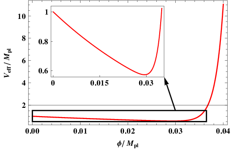
which is the key feature in the scenario under consideration. By setting the model parameters, it is possible to achieve minimum at late times such that the field rolls slowly around the minimum of the effective potential. The role of neutrino matter is solely related the transition to stable de Sitter around the present epoch. Fig. 1 shows the nature of the effective potential (52) and the inset shows the minimum of the effective potential.

Refer to caption — Figure 1: Effective potential (52) is plotted against the non-canonical field $\phi$ . $\tilde{\gamma}=30\;,\alpha=20\;,\hat{\rho}_{\nu}/M_{\textrm{Pl}}^{4}=10^{-10}\;{\rm and}\;\hat{p}_{\nu}/M_{\textrm{Pl}}^{4}=0$ are the chosen values of different parameters. Here we should note that if we change the values of the parameters $\hat{\rho}_{\nu}/M_{\textrm{Pl}}^{4}$ and $\hat{p}_{\nu}/M_{\textrm{Pl}}^{4}$ then the nature of the effective potential does not change and only the position of the minimum shifts along the horizontal axis. The inset shows the minimum of the effective potential.

Using Eq. (53) we get the minimum value of the effective potential (52) for $\phi=\phi_{\rm min}$ ,

\displaystyle V_{\rm eff,min}=\left(1+\frac{1}{\tilde{\gamma}}\right)V_{\rm min}\,,

(54)

where $V_{\rm min}=V(\phi_{\rm min})$ .

Eq. (54) can be represented in terms of the neutrino mass by using Eq. (50) and Eq. (51),

\displaystyle V_{\rm eff,min}=\left(1+\frac{1}{\tilde{\gamma}}\right)\left(\frac{m_{\nu}(z=0)}{m_{\nu,\rm min}}\right)^{1/\tilde{\gamma}}\mu^{2}M_{\textrm{Pl}}^{2}\,,

(55)

where $m_{\nu,\rm min}=m_{\nu}(\phi=\phi_{\rm min})$ .

Now $\mu\approx H_{0}$ [94] where $H_{0}$ is the present value of the Hubble parameter. So in Eq. (55) the term $\mu^{2}M_{\textrm{Pl}}^{2}\sim H_{0}^{2}M_{\textrm{Pl}}^{2}$ . If we take $H_{0}=70\rm kmMpc^{-1}sec^{-1}$ then we have in eV, $H_{0}=1.5\times 10^{-33}\rm eV$ . So $V_{\rm eff,min}$ will be of the order of $3H_{0}^{2}M_{\textrm{Pl}}^{2}$ only when,

\displaystyle\left(1+\frac{1}{\tilde{\gamma}}\right)\left(\frac{m_{\nu}(z=0)}{m_{\nu,\rm min}}\right)^{1/\tilde{\gamma}}\approx 1\,,

(56)

and since to get late time cosmic acceleration field has to settle down at the minimum of the effective potential during the present time we can safely take $m_{\nu}(z=0)=m_{\nu,\rm min}$ , which implies $\tilde{\gamma}\gg 1$ .

III.1 Canonical form of the action

Let us now transform the scalar-field part of the action (41) to its canonical form through the transformation

	$\displaystyle\sigma$	$\displaystyle=$	$\displaystyle\Bbbk(\phi)\,,$		(57)
	$\displaystyle k^{2}(\phi)$	$\displaystyle=$	$\displaystyle\left(\frac{\partial\Bbbk}{\partial\phi}\right)^{2}\,,$		(58)

where $k^{2}(\phi)$ is given by (42). Thus, (41) becomes

	$\displaystyle\mathcal{S}_{E}$	$\displaystyle=$	$\displaystyle\int d^{4}x\sqrt{g}\left[-\frac{M_{\textrm{Pl}}^{2}}{2}R+\frac{1}{2}\partial^{\mu}\sigma\partial_{\mu}\sigma+V(\Bbbk^{-1}(\sigma))\right]$		(59)
			$\displaystyle+\mathcal{S}_{m}+\mathcal{S}_{r}+\mathcal{S}_{\nu}(\mathcal{C}^{2}g_{\alpha\beta};\Psi_{\nu})\,,$		(59)

where $\mathcal{C}(\sigma)$ is the conformal coupling in the Einstein frame between the canonical field $\sigma$ and neutrinos. As we can see, the scalar field has now the canonical kinetic term.

The $\phi$ dependence of the canonical field $\sigma$ can be calculated from Eq. (58), and writes as

$\displaystyle\frac{\sigma(\phi)}{M_{\textrm{Pl}}}$	$\displaystyle=$	$\displaystyle\frac{\alpha\phi}{\tilde{\alpha}M_{\textrm{Pl}}}-\frac{1}{\tilde{\alpha}}\ln\left\{2\alpha^{2}+e^{\alpha\phi/M_{\textrm{Pl}}}\mu_{m}^{2}\left(\alpha^{2}+\tilde{\alpha}^{2}\right)\right.$	(60)
		$\displaystyle\left.+2\alpha\sqrt{\left(1+e^{\alpha\phi/M_{\textrm{Pl}}}\mu_{m}^{2}\right)\left(\alpha^{2}+e^{\alpha\phi/M_{\textrm{Pl}}}\mu_{m}^{2}\tilde{\alpha}^{2}\right)}\right\}$
		$\displaystyle+\frac{1}{\alpha}\ln\left\{\alpha^{2}+\tilde{\alpha}\left[\tilde{\alpha}+2e^{\alpha\phi/M_{\textrm{Pl}}}\mu_{m}^{2}\tilde{\alpha}\right.\right.$
		$\displaystyle\left.\left.+2\sqrt{\left(1+e^{\alpha\phi/M_{\textrm{Pl}}}\mu_{m}^{2}\right)\left(\alpha^{2}+e^{\alpha\phi/M_{\textrm{Pl}}}\mu_{m}^{2}\tilde{\alpha}^{2}\right)}\right]\right\}$
		$\displaystyle+C,~~~~~$

where $C$ is an integration constant. We consider $\sigma(\phi=0)=0$ ²² 2 The choice of $\sigma(\phi=0)$ also gives $\chi\to 0$ as $\sigma\to-\infty$ , similar to the $\phi$ field. Therefore, the value of $C$ we are getting here can also be obtained from Eq. (60) by putting $e^{\alpha\phi/M_{\textrm{Pl}}}=0$ and considering $\sigma(\chi\to 0)=\phi(\chi\to 0)$ ., which gives

	$\displaystyle C=\frac{1}{\tilde{\alpha}}\ln\left\{2\alpha^{2}+\mu_{m}^{2}\left(\alpha^{2}+\tilde{\alpha}^{2}\right)\right.$
	$\displaystyle\left.+2\alpha\sqrt{\left(1+\mu_{m}^{2}\right)\left(\alpha^{2}+\mu_{m}^{2}\tilde{\alpha}^{2}\right)}\right\}$
	$\displaystyle-\frac{1}{\alpha}\ln\left\{\alpha^{2}+\tilde{\alpha}\left[\tilde{\alpha}+2\mu_{m}^{2}\tilde{\alpha}\right.\right.$
	$\displaystyle\left.\left.+2\sqrt{\left(1+\mu_{m}^{2}\right)\left(\alpha^{2}+\mu_{m}^{2}\tilde{\alpha}^{2}\right)}\right]\right\}$		(61)

Additionally, if we consider $\tilde{\alpha}$ very small (according to [94] $\tilde{\alpha}\lesssim 0.02$ ) and $\alpha$ large comparing to $\tilde{\alpha}$ and $\mu_{m}$ [94], we can approximate it as

\displaystyle C\approx\frac{2}{\tilde{\alpha}}\ln\left(2\alpha\right)-\frac{2}{\alpha}\ln\left(\alpha+\tilde{\alpha}\right)\,.

(62)

Finally, note that in order to write the explicit form of $V(\sigma)=V(\Bbbk^{-1}(\sigma))$ in (59), we need to invert (60) in order to obtain the explicit form of $\phi(\sigma)$ , and then substitute into $V(\phi)$ in (46). However, (60) is a transcendental equation and thus it cannot be inverted. Fortunately, in the following elaboration $V(\sigma)$ will appear only through its derivative $dV(\sigma)/d\sigma$ , which using (57), (58) acquires the simple form

\displaystyle\frac{dV(\sigma)}{d\sigma}=\frac{1}{k(\phi)}\frac{dV(\phi)}{d\phi}.

(63)

In order to check whether the behavior of the field can comply with requirements spelled out in the aforesaid discussion, it would be convenient to check for the asymptotic behavior of the potential.

III.2 Asymptotic behavior

In the previous subsection we extracted the expressions for $\sigma(\phi)$ , $k(\phi)$ and $dV(\sigma)/d\sigma$ , where $\sigma$ is the redefined scalar field, in terms of which the action takes the canonical form. Since the involved expressions are quite complicated, it would be useful to obtain their asymptotic approximations. In particular, we are interested in the two limiting regimes, that is for small $\chi$ ( $\chi\ll m$ or equivalently $\phi\ll-2M_{\textrm{Pl}}\ln(\mu_{m})/\alpha$ ) and large $\chi$ ( $\chi\gg m$ or equivalently $\phi\gg-2M_{\textrm{Pl}}\ln(\mu_{m})/\alpha$ ) respectively.

For small $\chi$ from (31),(42) we have

k^{2}(\phi)\approx\frac{\alpha^{2}}{\tilde{\alpha}^{2}}\,,

(64)

and then Eq. (60) gives

\sigma(\phi)\approx\frac{\alpha}{\tilde{\alpha}}\phi\,.

(65)

Although, as we discussed in the end of the previous subsection, the explicit form of $V(\sigma)$ cannot be obtained, since it requires the inversion of the transcendental equation (60) of $\sigma(\phi)$ , its asymptotic form can be easily extracted, since now $\sigma(\phi)$ takes the simple form (65) which can be trivially inverted. In particular, for small $\chi$ the potential becomes

V_{s}(\sigma)\approx V_{s0}e^{-\tilde{\alpha}\sigma/M_{\textrm{Pl}}}\,.

(66)

which for small slope can facilitate slow roll which can continue for large values of $\chi$ . Similarly, for very large values of $\chi$ ( $\chi\gg m$ ), Eqs. (31),(42) lead to

\displaystyle k^{2}(\phi)\approx 1\,,

(67)

and then Eq. (60) gives

\displaystyle\sigma\approx\phi-\frac{2}{\tilde{\alpha}}\ln\left(\frac{\mu_{m}}{2}\right)+\frac{2}{\alpha}\ln\left(\frac{\tilde{\alpha}\mu_{m}}{\alpha+\tilde{\alpha}}\right)\,.

(68)

Thus, for large $\chi$ the potential reads

\displaystyle V_{l}(\sigma)\approx V_{l0}e^{-\alpha\sigma/M_{\textrm{Pl}}}\,.

(69)

which gives rise to scaling solution for $\alpha>\sqrt{3}$ , we shall take $\alpha\simeq 10$ to satisfy the nucleosynthesis constraint.

From the above asymptotic expressions, we deduce that the behavior of the canonical field $\sigma$ with respect to the non-canonical field $\phi$ , changes from a straight line with slope $\alpha/\tilde{\alpha}$ (for small $\phi$ ) to a straight line with slope 1, and $y$ axis intercepts at $-\frac{2}{\tilde{\alpha}}\ln\left(\frac{\mu_{m}}{2}\right)+\frac{2}{\alpha}\ln\left(\frac{\tilde{\alpha}\mu_{m}}{\alpha+\tilde{\alpha}}\right)$ (for large $\phi$ ). This behavior is always true as long as $\alpha>\tilde{\alpha}$ and $\alpha>\mu_{m}$ . In Fig. 2 we present the change in $\sigma$ -field behavior, in terms of the $\phi$ -field.

We next investigate the dynamics of unification in detail which includes inflationary phase,thermal history and late time cosmic acceleration. We shall also examine the issues related to relic gravity waves, a generic feature of the scenario under consideration. To this effect, we shall invoke the instant preheating to circumvent the excessive production of gravity waves.

IV Inflation

Having presented the scenario of variable gravity [94] in the Jordan and Einstein frames, in this section we proceed to a detailed investigation of the inflationary stage. As discussed earlier, at early times or equivalently for negative values/small positive values of the field, the potential $V(\phi)$ given by Eq. (46) reduces to the canonical potential $V_{s}(\sigma)$ of (66), which facilitates slow roll for small values of $\tilde{\alpha}\lesssim\sqrt{2}$ , where consistency with observations demands that $\tilde{\alpha}\ll 1$ . On the other hand, for very large values of $\phi$ , where $k(\phi)\to 1$ and the potential is given by (69), we obtain the required scaling behavior in radiation and matter era, for $\alpha\gtrsim 10$ .

The $\sigma$ -field slow roll parameters, can be easily expressed in terms of $\phi$ as

	$\displaystyle\epsilon$	$\displaystyle=$	$\displaystyle\frac{M_{\textrm{Pl}}^{2}}{2}\left(\frac{1}{V}\frac{{\rm d}V}{{\rm d}\sigma}\right)^{2}=\frac{M_{\textrm{Pl}}^{2}}{2k^{2}(\phi)}\left(\frac{1}{V}\frac{{\rm d}V}{{\rm d}\phi}\right)^{2}=\frac{\alpha^{2}}{2k^{2}(\phi)}\,,~~~~\,\,$		(70)
	$\displaystyle\eta$	$\displaystyle=$	$\displaystyle\frac{M_{\textrm{Pl}}^{2}}{V}\frac{{\rm d^{2}}V}{{\rm d}\sigma^{2}}=2\epsilon-\frac{M_{\textrm{Pl}}}{\alpha}\frac{{\rm d}\epsilon(\phi)}{{\rm d}\phi}\ ,$		(71)

where we have made use of (63). Since $\alpha^{2},\tilde{\alpha}^{-2}\gg 1$ , the slow-roll regime lasts for large values of $\phi$ (since $k^{2}=\alpha^{2}/2$ ) such that $X\equiv\mu^{2}/m^{2}e^{\alpha\phi/M_{p}}\gg 1$ , and thereafter the field crosses to the kinetic regime where $k\simeq 1$ .

Clearly, the large-field slow-roll regime is of great physical interest. In this case the slow-roll parameters are simplified to

\displaystyle\epsilon=\eta=\frac{\tilde{\alpha}^{2}}{2}X\ \to\ X_{\rm end}=\frac{2}{\tilde{\alpha}^{2}}

(72)

and the kinetic function is given by

k^{2}(\phi)\simeq\frac{\alpha^{2}}{\tilde{\alpha}^{2}X}\ \to\ k_{\rm end}\simeq\frac{\alpha}{\sqrt{2}}.

(73)

We mention that $k^{2}$ interpolates between $\alpha/\tilde{\alpha}$ and $1$ , as the field evolves from early epochs to late times. At the end of inflation $k_{\rm end}\simeq 6$ , and then it quickly relaxes to $k=1$ marking the beginning of the kinetic regime. This transition takes place very fast, since the kinetic function decreases exponentially with the field.

It is convenient to express the physical quantities in terms of the non-canonical field $\phi$ too. It is then straightforward to write down the Friedman equation in slow-roll regime as

H^{2}=\frac{M_{\textrm{Pl}}^{2}}{3}e^{-\alpha\phi/M_{\textrm{Pl}}}\equiv\frac{\mu^{2}}{3m^{2}}\frac{M_{\textrm{Pl}}^{2}}{X},

(74)

which we shall use in the following discussion.

The Number of efoldings are given by,

$\displaystyle\mathcal{N}(\phi)$	$\displaystyle=$	$\displaystyle\frac{1}{\alpha M_{\textrm{Pl}}}\int_{\phi}^{\phi_{\rm end}}k^{2}(\phi){\rm d}\phi^{\prime}\,,$	(75)
	$\displaystyle=$	$\displaystyle\frac{\alpha\left(\phi_{\rm end}-\phi\right)}{\tilde{\alpha}^{2}}$
		$\displaystyle+\left(\frac{1}{\alpha^{2}}-\frac{1}{\tilde{\alpha}^{2}}\right)\ln\left(\frac{m^{2}+\mu^{2}e^{\alpha\phi_{\rm end}/M_{\textrm{Pl}}}}{m^{2}+\mu^{2}e^{\alpha\phi/M_{\textrm{Pl}}}}\right)\,,~~~~~$

Where $\phi{\rm end}$ is the value of $\phi$ field at the end of inflation. Now from Eq. (72) we have $e^{\alpha\phi_{\rm end}/M_{\textrm{Pl}}}=2m^{2}/(\tilde{\alpha}^{2}\mu^{2})$ which approximates the Eq. (75) by neglecting $\alpha^{-2}$ term with respect to $\tilde{\alpha}^{-2}$ ,

\displaystyle\mathcal{N}(\phi)

\displaystyle\approx

\displaystyle\frac{1}{\tilde{\alpha}^{2}}\Bigg[\ln\left(1+X^{-1}\right)-\ln\left(1+\frac{\tilde{\alpha}^{2}}{2}\right)\Bigg].~~~~~

(76)

Fo given efoldings from Eq. (76) we can calculate the value of $\phi$ when inflation started.

The number of e-foldings in the large- $X$ approximation are given by

\displaystyle\mathcal{N}(\phi_{\rm in})\simeq\frac{1}{\tilde{\alpha}^{2}X_{\rm in}}\,,

(77)

where $\phi_{\rm in}$ designates the field-value where inflation commences. The COBE normalized value of density perturbations [118, 119]

\delta^{2}_{H}=\frac{1}{150\pi^{2}}\frac{1}{M_{\textrm{Pl}}^{4}}\frac{V_{\rm in}}{\epsilon}\simeq 2\times 10^{-10}\,,

(78)

then allows us to estimate $V_{\rm in}$ as well as the important ratio of parameters, $\tilde{\alpha}^{2}\mu^{2}/m^{2}$ in terms of the number of e-foldings, namely

	$\displaystyle\frac{\tilde{\alpha}^{2}\mu^{2}}{m^{2}}=\frac{150\times\pi^{2}\times 10^{-10}}{\mathcal{N}^{2}}$		(79)
	$\displaystyle V_{\rm in}=\mathcal{N}\frac{\tilde{\alpha}^{2}\mu^{2}}{m^{2}}M_{\textrm{Pl}}^{4}=\frac{150\times\pi^{2}\times 10^{-10}}{\mathcal{N}}M_{\textrm{Pl}}^{4}\,.$		(80)

Let us also note the important relationship between $H_{\rm in}$ and $H_{\rm end}$ using the expressions of $X_{\rm in}$ and $X_{\rm end}$ :

\frac{H^{2}_{\rm end}}{H^{2}_{\rm in}}=\frac{V_{\rm end}}{V_{\rm in}}=\frac{X_{\rm in}}{X_{\rm end}}=\frac{1}{2\mathcal{N}}\,,

(81)

which in particular can be used to estimate the Hubble parameter at the end of inflation:

H^{2}_{\rm end}=\frac{M_{\textrm{Pl}}^{2}}{6}\frac{\tilde{\alpha}^{2}\mu^{2}}{m^{2}}=\frac{25\pi^{2}\times 10^{-10}}{\mathcal{N}^{2}}M_{\textrm{Pl}}^{2}\,.

(82)

As mentioned in the introduction, the scenario under consideration does not belong to the class of oscillatory models. In this case we need to look for an alternative reheating mechanism, and a possible candidate is the gravitational particle production [65, 66]. The space time geometry undergoes a crucial transition at the end of inflation, involving essentially a non-adiabatic process that gives rise to particle production. Assuming thermalization of the so produced energy, the energy density of radiation produced in this process at the end of inflation is given by

\rho_{\rm rad}\simeq 0.01\times g_{p}H_{\rm end}^{4}\,,

(83)

where $g_{p}$ is the number of different species produced at the end of inflation, varying typically between 10 and 100. Thus, assuming $g_{p}\sim 100$ , we obtain the radiation temperature

T_{\rm end}\simeq 1.5\times\frac{10^{-4}}{\mathcal{N}}M_{\textrm{Pl}}\,.

(84)

Up to now we have kept the number of e-foldings arbitrary. This number typically depends upon the reheating temperature and also the scale of inflation. It can be estimated by considering a typical length scale which leaves the Hubble scale during inflation at $a=a_{\rm in}$ and re-enters the horizon today:

	$\displaystyle k=a_{\rm in}H_{\rm in}=a_{0}H_{0}\to\frac{k}{a_{0}H_{0}}=\frac{a_{\rm in}}{a_{\rm end}}\frac{a_{\rm end}}{a_{0}}\frac{H_{\rm in}}{H_{0}}$
	$\displaystyle=e^{-\mathcal{N}}\frac{T_{0}}{T_{\rm end}}\frac{H_{\rm in}}{H_{0}}\,,$		(85)

which gives $\mathcal{N}\simeq 70$ . Therefore, the temperature at the end of inflation is given by

\displaystyle T_{\rm end}\simeq 3.6\times 10^{12}\rm GeV.

(86)

We then estimate the spectral index $n_{s}$ and the ratio of tensor-to-scalar perturbations $r$ as

	$\displaystyle n_{s}\approx 1-6\epsilon+2\eta=1-\frac{2}{\mathcal{N}}\simeq 0.97\,,$		(87)
	$\displaystyle r\approx 16\epsilon=\frac{8}{\mathcal{N}}\simeq 0.11\,.$		(88)

Eq. (87) and Eq. (88) can be combined in a single equation, namely

\displaystyle r=4\left(1-n_{s}\right)\,.

(89)

In Fig. 3 we present the $68\%$ and $95\%$ contours on $n_{s}-r$ plane, using the data of $Planck+WP+BAO$ [120]. On top of them we depict the $n_{s}$ and $r$ values calculated in our model using (87) and (88) respectively, having considered the e-foldings $(\mathcal{N})$ between 55 and 70. It seems that the value $\mathcal{N}=55$ is ruled out upto 2 $\sigma$ level for this model. But the values slightly higher than 55 are well within the 2 $\sigma$ level. The line shown in the Fig. 3 follows Eq. (89).

In the subsection to follow, we consider the problem related to excessive production of relic gravity waves.

IV.1 Relic gravity waves and nucleo-synthesis constraint on reheating temperature

Let us assume that gravitational particle production is the sole mechanism for reheating [61, 63, 64, 65, 66, 62, 67, 68]. In this case using Eqs. (74) and (83) and considering $\mathcal{N}=70$ we have,

\left(\frac{\rho_{\phi}}{\rho_{r}}\right)_{\rm end}\simeq\frac{M_{\textrm{Pl}}^{2}H^{2}_{\rm end}}{0.01\times g_{p}H^{4}_{\rm end}}\simeq 2\times 10^{11};(g_{p}\simeq 100)\,.

(90)

This ratio is typically $10^{16}$ in braneworld models [27, 28]. Hence, it takes long for the radiative regime to commence. In those models similar to our situation potential is very steep after inflation and therefore $\rho_{\phi}\sim 1/a^{6}$ till radiation takes over. During this regime called kinetic regime the gravity wave(produced during inflation) amplitude enhances and violates nucleosynthesis constraints at the commencement of the radiative regime [27, 28]. We have to check it here also.

The quantum mechanical production of gravity waves during inflation is a generic feature of the scenario. The tensor perturbations $h_{ij}$ satisfy the Klein-Gordon equation $\Box h_{ij}=0$ [69, 70] which gives,

\ddot{\varphi}_{k}(\tau)+2\frac{\dot{a}}{a}\varphi_{k}(\tau)+k^{2}\varphi_{k}(\tau)=0\,,

(91)

where $h_{ij}\sim\varphi_{k}e^{ikx}e_{ij}$ ( $e_{ij}$ is polarization tensor); $\tau$ ( ${\rm d}\tau={\rm d}t/a$ ) is conformal time and $k$ is comoving wave number. As pointed out in the preceding discussion, inflation is approximately exponential thereby $a=\tau_{0}/\tau$ and $H_{\rm in}=-1/\tau_{0}$ is the Hubble parameter during inflation. The “in” state $\varphi_{\rm in}^{(+)}(k,\tau)$ corresponds to the positive frequency solution of Eq. (91) in the adiabatic vacuum( $\varphi_{\rm in}^{(+)}(k,\tau)=(\pi\tau_{0}/4)^{1/2}(\tau/\tau_{0})^{3/2}H^{(2)}_{3/2}(k\tau)$ . After inflation has ended, universe from quasi de Sitter phase makes transition to the phase characterized by power law expansion. In the standard scenario, the post inflationary evolution is described by radiative regime whereas in the quintessential inflation, the after inflation transition is to kinetic phase with stiff equation of state parameter [27, 28]. This transition involves non-adiabatic change of geometry. We shall assume that post inflationary dynamics is described by power law expansion, $a=(t/t_{0})^{p}\equiv(\tau/\tau_{0})^{1/2-\mu}$ where $\mu\equiv 3/2((w-1)/(3w+1))$ with $w$ being the post inflationary equation of state parameter. Let us notice that $\mu=0$ in kinetic regime( $w=1$ ). The ”out” state contains both positive and negative frequency solutions to (91),

\varphi_{\rm out}=\alpha\varphi_{\rm out}^{(+)}+\beta\varphi_{\rm out}^{(-)}\,,

(92)

where $\alpha$ and $\beta$ are Bogoliubov coefficients [27]. The ”out” is state is given by, $\varphi^{(+,-)}_{\rm out}=(\pi\tau_{0}/4)^{1/2}(\tau/\tau_{0})^{\mu}H^{(2,1)}_{|\mu|}(k\tau)$ . The energy density of relic gravity waves depends upon $\beta$ [27, 72],

\rho_{g}=<T_{00}>=\frac{1}{\pi^{2}a^{2}}\int{{\rm d}kk^{3}|\beta|^{2}}\,.

(93)

During kinetic regime, $|\beta_{\rm kin}|^{2}\sim(k\tau_{\rm kin})^{-3}$ , as a result using (93), we obtain,

\rho_{g}=\frac{32}{3\pi}h^{2}_{\rm GW}\rho_{b}\left(\frac{\tau}{\tau_{\rm kin}}\right)

(94)

where $\rho_{b}$ is the background energy density made by radiation and scalar stiff matter. While deriving (94), we made use of the fact that $H_{\rm in}=-1/\tau_{0}$ . Since, at radiation, field equality ( $\tau=\tau_{\rm eq}$ ), $\tau_{\rm eq}/\tau_{\rm kin}=(T_{\rm kin}/T_{\rm eq})^{2}$ and $\rho_{b}=2\rho_{r}$ , we have from Eq. (94),

\left(\frac{\rho_{g}}{\rho_{r}}\right)_{\rm eq}=\frac{64}{3\pi}h^{2}_{\rm GW}\left(\frac{T_{\rm end}}{T_{\rm eq}}\right)^{2}\,,

(95)

where $h_{\rm GW}$ is the dimensionless gravity amplitude which needs to be fixed in each model imposing COBE normalization [119, 118],

	$\displaystyle h^{2}_{\rm GW}$	$\displaystyle=$	$\displaystyle\frac{H^{2}_{\rm in}}{8\pi M_{\textrm{Pl}}^{2}}=\frac{\mathcal{N}}{24\pi}\left(\frac{\tilde{\alpha}^{2}\mu^{2}}{m^{2}}\right)=\frac{\mathcal{N}}{4\pi}\frac{H^{2}_{\rm end}}{M_{\textrm{Pl}}^{2}}$		(96)
			$\displaystyle\simeq 2.8\times 10^{-11}\,.$		(96)

Let us notice from (95) that longer is the kinetic regime smaller would be $T{\rm eq}$ thereby larger would be the ratio of energy densities of relic gravity waves and radiation at equality. It may also be worthwhile to note from (93) that $\rho_{g}\sim 1/a^{4}$ for $\omega>1/3$ whereas $\rho_{g}\sim\rho_{b}$ if $\omega<1/3$ and during radiation era also $\rho_{g}$ approximately tracks the background. It is the specific behavior of $\rho_{g}$ during kinetic regime which causes problem.

For simplicity we shall here made an approximation that the field after inflation instantaneously come to kinetic regime( $\rho_{\phi}\sim 1/a^{6}$ ). In fact, $\rho_{\phi}\sim 1/a^{2}$ at $\phi=\phi_{\rm end}$ and soon thereafter, the field enters the kinetic regime which happens pretty fast as potential is steep. Thus we shall assume that $H_{\rm end}\simeq H_{\rm kin}$ and $T_{\rm end}\simeq T_{\rm kin}$ . Numerical calculations show that kinetic regime fast commences, (see Fig. 4) after the end of inflation; our estimates do not change significantly by adopting the said approximation. Since $T_{\rm eq}\sim T_{\rm end}/a_{\rm eq}$ , we have,

\left(\frac{\rho_{\phi}}{\rho_{r}}\right)_{\rm end}=\left(\frac{T_{\rm end}}{T_{\rm eq}}\right)^{2}

(97)

we have the following relation,

\left(\frac{\rho_{\phi}}{\rho_{r}}\right)_{\rm end}=\frac{3\pi}{64}\left(\frac{\rho_{g}}{\rho_{r}}\right)_{\rm eq}\frac{1}{h^{2}_{\rm GW}}\,.

(98)

As for $\rho_{g}/\rho_{r}$ at equality, nucleosynthesis dictates that it should be less than $0.2$ [27]. We know left hand side, so if we estimate gravity wave amplitude, we can find out whether the gravitational particle production can do the job. Indeed, we find using Eq.(96),

\left(\frac{\rho_{\phi}}{\rho_{r}}\right)_{\rm end}\lesssim\frac{3\pi}{64}\times 0.2\times\frac{4\pi}{\mathcal{N}}\frac{M_{\textrm{Pl}}^{2}}{H^{2}_{\rm end}}\simeq 10^{9}\,.

(99)

Comparing the estimate with the one obtained by using (90), we conclude that even if we take $g_{p}\sim 100$ , the gravitational particle production does not meet the requirement imposed by the nucleosynthesis constraint at the commencement of radiative regime. It should also be noted that kinetic regime does not set instantaneously; incorporating evolution from the end of inflation to the beginning of kinetic regime further worsens the situation. Gravitational particle production is clearly an inefficient process and we should therefore look for an alternative way of reheating. Instant preheating provides with an efficient mechanism which suits to the quintessential inflation scenario under consideration.

Let us also quote the spectral energy density of the gravitational wave (see Ref.[27] for details),

\Omega_{\rm GW}(\lambda)=\frac{1}{\rho_{c}}\frac{{\rm d}\rho_{g}}{{\rm d}\ln k}\,,

(100)

where $\rho_{c}$ is the critical energy density.

In different epochs, the form of $\Omega_{\rm GW}$ is given by,

	$\displaystyle\Omega_{\rm GW}^{\rm(MD)}=\frac{3}{8\pi^{3}}h_{\rm GW}^{2}\Omega_{m0}\left(\frac{\lambda}{\lambda_{h}}\right)^{2}\,,\lambda_{\rm MD}<\lambda\leq\lambda_{h},~~~~~~$		(101)
	$\displaystyle\Omega_{\rm GW}^{\rm(RD)}(\lambda)=\frac{1}{6\pi}h_{\rm GW}^{2}\Omega_{r0},~~~~~~~~~\lambda_{\rm RD}<\lambda\leq\lambda_{\rm MD}\,,~~~~~$		(102)
	$\displaystyle\Omega_{\rm GW}^{\rm(kin)}(\lambda)=\Omega_{\rm GW}^{\rm(RD)}\left(\frac{\lambda_{\rm RD}}{\lambda}\right)\,,~~~~~\lambda_{\rm kin}<\lambda\leq\lambda_{\rm RD}\,,~~~~~$		(103)

where,

$\displaystyle\lambda_{h}$	$\displaystyle=$	$\displaystyle 2cH_{0}^{-1}\,,$	(104)
$\displaystyle\lambda_{\rm MD}$	$\displaystyle=$	$\displaystyle\frac{2\pi}{3}\lambda_{h}\left(\frac{\Omega_{r0}}{\Omega_{m0}}\right)^{1/2}\,,$	(105)
$\displaystyle\lambda_{\rm RD}$	$\displaystyle=$	$\displaystyle 4\lambda_{h}\left(\frac{\Omega_{m0}}{\Omega_{r0}}\right)^{1/2}\frac{T_{\rm MD}}{T_{\rm rh}}\,,$	(106)
$\displaystyle\lambda{\rm kin}$	$\displaystyle=$	$\displaystyle cH_{\rm kin}^{-1}\left(\frac{T_{\rm rh}}{T_{0}}\right)\left(\frac{H_{\rm kin}}{H_{\rm rh}}\right)^{1/3}\,,$	(107)

where “MD”, “RD” and “kin” represent matter dominated, radiation dominated and kinetic energy dominated epochs and $\lambda$ represents wavelength. $H_{0}$ is the present value of Hubble parameter and $\Omega_{m0}$ and $\Omega_{r0}$ are the present values of matter and radiation energy densities. $T_{\rm rh}$ and $H_{\rm rh}$ are the reheating temperature and Hubble parameter respectively which are approximately same as the temperature and Hubble parameter at the end of the inflation respectively.

IV.2 Instant preheating

In this subsection, we shall describe instant preheating applied to the scenario under consideration. We shall demonstrate its viability to tackle the problem associated with relic gravity waves.

Inflation ends when $\phi=\phi_{\rm end}$ which, for convenience, we can shift to the origin by translating the field, $\phi^{\prime}=\phi-\phi_{\rm end}$ without the loss of generality. In what follows we would keep using $\phi$ remembering that the translated field $\phi<0$ . We next assume that $\phi$ interacts with a new field $\chi$ which interacts with a Fermi field via Yukawa interaction,

\mathcal{L}_{\rm int}=-\frac{1}{2}g^{2}\phi^{2}\chi^{2}-h\bar{\psi}\psi\chi

(108)

where $\chi$ does not have bare mass, its effective mass is given by, $m_{\chi}=g|\phi|$ and couplings $g$ $\&$ $h$ are assumed to be positive. In the model under consideration, the field $\phi$ soon comes to kinetic regime after inflation has ended as potential is steep there. In this case the production of $\chi$ particles may commence provided $m_{\chi}$ changes non-adiabatically [89, 90],

\dot{m}_{\chi}\gtrsim m^{2}_{\chi}\to\dot{\phi}\gtrsim g\phi^{2}\,.

(109)

The condition for particle production (109) can be satisfied provided,

|\phi|\lesssim|\phi_{p}|=\sqrt{\frac{\dot{\phi}_{\rm end}}{g}}\,.

(110)

Using slow roll equations (70) and (71), it can be noticed that,

\dot{\phi}_{\rm end}=\frac{\alpha}{k_{\rm end}^{2}}\sqrt{\frac{V_{\rm end}}{3}};~~k_{\rm end}=\frac{\alpha}{\sqrt{2}}\,.

(111)

Since $\phi_{p}\lesssim M_{\textrm{Pl}}$ , from Eq. (110) we have a constraint on the coupling $g$ ,

\frac{\dot{\phi}_{\rm end}}{g}\lesssim M_{\textrm{Pl}}^{2}\to g\gg\frac{2}{\alpha M_{\textrm{Pl}}^{2}}\sqrt{\frac{V_{\rm end}}{3}}\,.

(112)

Further, we can estimate the production time,

\delta{t}_{p}\sim\frac{|\phi|}{\dot{\phi}}=g^{-1/2}\dot{\phi}_{\rm end}^{-1/2}\,.

(113)

Using then uncertainty relation gives us the estimate for wave number, $k_{p}\simeq\delta{t}^{-1}_{p}\simeq\sqrt{g\dot{\phi}_{\rm end}}$ . We then can find out the occupation number for $\chi$ particles [90, 62],

n_{k}\sim e^{-\pi k^{2}/k^{2}_{p}}\,,

(114)

which gives the number density of $\chi$ particle,

N_{\chi}=\frac{1}{(2\pi)^{3}}\int_{0}^{\infty}{n_{k}d^{3}{\bf k}}=\frac{(g\dot{\phi}_{\rm end})^{3/2}}{(2\pi)^{3}}\,.

(115)

The energy density of created particles $\chi$ is given by,

\displaystyle\rho_{\chi}=N_{\chi}m_{\chi}=\frac{(g\dot{\phi}_{\rm end})^{3/2}}{(2\pi)^{3}}g|\phi_{p}|=\frac{g^{2}V_{\rm end}}{6\pi^{3}\alpha^{2}}\,.

(116)

If the particle energy produced at the end of inflation is supposed to be thermalized then using Eq. (74) and Eq. (116) we find,

\left(\frac{\rho_{\phi}}{\rho_{r}}\right)_{\rm end}\simeq\frac{6\pi^{3}\alpha^{2}}{g^{2}}

(117)

Using (117), we can find lower limit on the coupling $g$ by invoking the relic gravity constraint on $\rho_{\phi}/\rho_{r}$ from (99),

g\gtrsim 6\alpha\times 10^{-5}

(118)

Let us further note that

	$\displaystyle\delta t_{p}H_{\rm end}\simeq\sqrt{\frac{\alpha}{2gM_{\textrm{Pl}}^{2}}}\left(\frac{V_{\rm end}}{3}\right)^{1/4}<\frac{4.5\times 10^{-5/2}}{\mathcal{N}}$
	$\displaystyle\Rightarrow\delta t_{p}\ll H^{-1}_{\rm end}\,,$		(119)

since $\mathcal{N}\sim 70$ . This tells us that during particle production expansion can be ignored. Let us also notice that $\phi_{p}\simeq 4\times 10^{-4}$ which implies that particle production takes place all most instantaneously after inflation has ended. Since $\phi$ runs fast after inflation has ended, the mass of $\chi$ grows larger making it to decay into $\bar{\psi}\psi$ , the decay width is given by

\Gamma_{\bar{\psi}\psi}=\frac{h^{2}m_{\chi}}{8\pi}=\frac{h^{2}}{8\pi}g|\phi|

(120)

We should now worry about the back reaction of $\chi$ on the post inflationary dynamics of $\phi$ . Around $\phi=0$ where inflation ends, $\rho_{\phi}\sim 1/a^{2}$ thereby the field potential as well as the dissipative term in the evolution equation for $\phi$ evolve slower than $\rho_{\chi}$ . On the other hand, the decay rate is larger of larger values of $\phi$ as $m_{\chi}$ gets larger. Hence, the decay of $\chi$ into Fermions would be accomplished before the back reaction of $\chi$ on $\phi$ evolution becomes important provided that,

\Gamma_{\bar{\psi}\psi}\gg H_{\rm end}\to h^{2}\gtrsim 8\pi\frac{H_{\rm end}}{g|\phi|}

(121)

Since $\phi\lesssim M_{\textrm{Pl}}$ , the above estimate implies that $h\gtrsim 2g^{-1/2}\times 10^{-6}$ which gives the lower bound on the numerical value of the coupling $h$ . Fig. 5 shows the allowed values of $g$ and $h$ . It is clear that is a wide region in the parameter space where the instant preheating is quite efficient.

Fig. 6 shows the spectral energy density ( $\Omega_{\rm GW}$ ) of relic gravitational wave background along with the sensitivity curve of AdvLIGO [121, 122] and LISA [123, 124]. To plot Fig. 6 we have taken the present values of matter and radiation energy density to be 0.3 and $9\times 10^{-5}$ respectively.

Next, we turn to late time dynamics of the model.

V Late time Cosmology: Dark Energy

In this section we investigate the cosmological behavior at late times, where as we mentioned in the Introduction the scenario at hand leads to an effective dark energy driving universe acceleration.

V.1 Evolution equations

We consider the spatially flat Friedmann-Robertson-Walker (FRW) cosmology,

\displaystyle ds^{2}=-N^{2}dt^{2}+a(t)^{2}\delta_{ij}dx^{i}dx^{j}~,

(122)

Varying the action (59) with respect to the metric $g_{\mu\nu}$ and setting $N=1$ , we obtain the two Friedmann equations:

	$\displaystyle 3H^{2}M_{\textrm{Pl}}^{2}=\frac{1}{2}\dot{\sigma}^{2}+V(\sigma)+\rho_{m}+\rho_{r}+\rho_{\nu}\,,$		(123)
	$\displaystyle\left(2\dot{H}+3H^{2}\right)M_{\textrm{Pl}}^{2}=-\frac{1}{2}\dot{\sigma}^{2}+V(\sigma)-\frac{1}{3}\rho_{r}-p_{\nu},\,~~~~~~$		(124)

where, as we mentioned, the neutrino pressure $p_{\nu}$ behaves as radiation during the early times but it behaves like non-relativistic matter during the late times. Varying the action (59) with respect to the field $\sigma$ leads to its equation of motion ³³ 3 Variation of $\mathcal{S}_{\nu}$ with respect to $\sigma$ reads as $\displaystyle\frac{1}{\sqrt{-g}}\frac{\delta\mathcal{S}_{\nu}}{\delta\sigma}=\frac{1}{\sqrt{-g}}\frac{\delta\mathcal{S}_{\nu}}{\delta\phi}\frac{\partial\phi}{\partial\sigma}=\frac{\mathcal{C}_{,\phi}}{\mathcal{C}}\frac{T^{(\nu)}}{k(\phi)}\,.$ :

\displaystyle\ddot{\sigma}+3H\dot{\sigma}=-\frac{{\rm d}V(\sigma)}{{\rm d}\sigma}-\frac{\partial\ln m_{\nu}}{\partial\sigma}\left(\rho_{\nu}-3p_{\nu}\right)\,.

(125)

Additionally, note that relation (50), using (57) and (58), gives

\displaystyle\frac{\partial\ln m_{\nu}}{\partial\sigma}=\frac{\tilde{\gamma}\alpha}{M_{\textrm{Pl}}k(\phi)}\,.

(126)

Let us make an important comment here. During radiative regime, the last term in the r.h.s. of Eq. (125) does not contribute as during that era neutrinos behave like radiation and the energy momentum tensor is traceless. On the contrary, at late times, neutrinos behave as non-relativistic matter. As a result, the last term in the r.h.s. of (125) is non-zero and the non-minimal coupling between the scalar field and the neutrinos builds up which plays a vital role in the model under consideration.

According to [94], as we mentioned in (67), during and after radiation era, we can take $\chi\gg m$ and $k(\phi)\approx 1$ . Thus, the neutrino mass (50) at late times exhibits an effective behavior

\displaystyle m_{\nu,\rm eff}(\sigma)=m_{\nu,0}e^{\tilde{\gamma}\alpha\sigma/M_{\textrm{Pl}}}\,,

(127)

which shows the same behavior as Eq. (50) that gives rise to the same type of effective potential like Eq. (52). In this case, the neutrino conservation equation (49) effectively reads

\displaystyle\dot{\rho}_{\nu}+3H(\rho_{\nu}+p_{\nu})=\frac{\tilde{\gamma}\alpha}{M_{\textrm{Pl}}}\dot{\sigma}(\rho_{\nu}-3p_{\nu})\,.

(128)

We stress here that in the scenario at hand, the late-time acceleration is attributed to the combined effect of neutrinos and scalar field, that is the effective dark energy sector includes these two contributions, namely its energy density and pressure read

	$\displaystyle\rho_{\rm DE}\equiv\rho_{\nu}+\rho_{\sigma}=\rho_{\nu}+\frac{1}{2}\dot{\sigma}^{2}+V(\sigma),$		(129)
	$\displaystyle p_{\rm DE}\equiv p_{\nu}+p_{\sigma}=p_{\nu}+\frac{1}{2}\dot{\sigma}^{2}-V(\sigma),$		(130)

and they obey the continuity equation

\displaystyle\dot{\rho}_{\rm DE}+3H\left(\rho_{\rm DE}+p_{\rm DE}\right)=0\,.

(131)

There is still one missing information in order for the above cosmological equations to close, namely the behavior of the neutrino equation-of-state parameter $w_{\nu}\equiv p_{\nu}/\rho_{\nu}$ , which determines the neutrino pressure $p_{\nu}$ that enters into $p_{\rm DE}$ , and then into the conservation equation (131).

As we discussed in detail in section (III), before and during the radiation era neutrinos are relativistic and behave as radiation, while during and after the matter era neutrinos become non-relativistic and $w_{\nu}$ becomes $0$ . Thus, a complete and detailed investigation of the thermal history of the universe requires the exact behavior of $w_{\nu}$ , that is its specific form interpolating between these two regimes. Expressing the universe evolution through the redshift $z$ , for convenience, one can have several $w_{\nu}(z)$ parameterizations with the above required properties, namely, the interpolation of the equation of state parameter between $1/3$ $\&$ $0$ [114]. In this work we desire to have a better control on the features of this transition, namely, the epoch around which the transition is realized and the duration of realization. We shall use the following ansatz for $w_{\nu}(z)$ ,

\displaystyle w_{\nu}(z)=\frac{p_{\nu}}{\rho_{\nu}}=\frac{1}{6}\left\{1+\tanh\left[\frac{\ln(1+z)-z_{\rm eq}}{z_{\rm dur}}\right]\right\}\,.

(132)

In the above expression $z_{\rm eq}$ determines the moment around which the transition takes place; the choice for the transition redshift where matter and radiation energy densities become equal is reasonable. Additionally, $z_{\rm dur}$ determines how fast this transition is realized. In particular, having in mind that varying mass, neutrinos become non-relativistic after their mass turns constant [100, 101], and imposing the physical requirement that the varying mass of neutrinos has to be non-relativistic at the recent cosmological past, we deduce that we need a large value of $z_{\rm dur}$ such that the transition is smooth. However, the exact $z_{\rm dur}$ -determination requires exact knowledge of the redshift $z_{\rm NR}$ after which neutrinos become non-relativistic, which according to [100, 101] is $z_{\rm NR}\in(2-10)$ for $m_{\nu}\in(0.015-2.3)$ , while according to [113] it is $z_{\rm NR}<4$ .

Finally, in order to compare with observations, we introduce the dimensionless density parameters for radiation, matter, neutrinos and scalar field, respectively as

$\displaystyle\Omega_{m}$	$\displaystyle=$	$\displaystyle\frac{\rho_{m}}{3H^{2}M_{\textrm{Pl}}^{2}}\,,$	(133)
$\displaystyle\Omega_{r}$	$\displaystyle=$	$\displaystyle\frac{\rho_{r}}{3H^{2}M_{\textrm{Pl}}^{2}}\,,$	(134)
$\displaystyle\Omega_{\nu}$	$\displaystyle=$	$\displaystyle\frac{\rho_{\nu}}{3H^{2}M_{\textrm{Pl}}^{2}}\,,$	(135)
$\displaystyle\Omega_{\sigma}$	$\displaystyle=$	$\displaystyle\frac{\rho_{\sigma}}{3H^{2}M_{\textrm{Pl}}^{2}}\,.,$	(136)

and thus, according to (129),

\displaystyle\Omega_{\rm DE}=\Omega_{\sigma}+\Omega_{\nu}\,.

(137)

Lastly, the equation-of-state parameters of the total matter content in the universe of the scalar-field sector and of the dark-energy sector can be written as

$\displaystyle w_{\rm eff}$	$\displaystyle=$	$\displaystyle-1-\frac{2}{3}\frac{\dot{H}}{H^{2}},$	(138)
$\displaystyle w_{\sigma}$	$\displaystyle=$	$\displaystyle\frac{p_{\sigma}}{\rho_{\sigma}}\,,$	(139)
$\displaystyle w_{\rm DE}$	$\displaystyle=$	$\displaystyle\frac{w_{\rm eff}-\frac{1}{3}\Omega_{r}}{\Omega_{\rm DE}}\,.$	(140)

In what follows we shall present our numerical results.

V.2 Post inflationary dynamics: the epoch sequence

Let us not examine the thermal history of the universe, that is we are interesting in its transient behavior from inflation to the present epoch. Due to the complexities of the cosmological equations of the previous subsection, no exact analytical solutions are possible and one needs to perform a numerical elaboration. In particular, we numerically evolve the cosmological equations (123), (124), (125),(126), (131),(132), focusing on the evolution of observables like the various density and equation-of-state parameters. For the numerical evolution we consider $\alpha=10$ , $\tilde{\gamma}=30$ and⁴⁴ 4 The parameter $\tilde{\gamma}$ enters in the expression of the minimum of the effective potential (52) given by $V_{\rm eff,min}=\left(1+1/\tilde{\gamma}\right)V_{\rm min}$ which tells us that $\tilde{\gamma}\gg 1$ for $V_{\rm eff,min}\sim H_{0}^{2}M_{\textrm{Pl}}^{2}$ . $\tilde{\gamma}$ also enters in the expression of equation of state parameter of dark energy whose value at the attractor point is given by $w_{\rm DE}=-\tilde{\gamma}/(1+\tilde{\gamma})$ . There is nothing special about $\tilde{\gamma}=30$ . It could be any large value such that $w_{\rm DE}$ falls within the observed value of the equation of state parameter(For instance, $\tilde{\gamma}=30$ . $w_{\rm DE}\approx 0.97$ ). $z_{\rm dur}=3.6$ and $10$ , and for the initial conditions of the radiation and scalar field we use the ratio of $\rho_{r}$ and $\rho_{\sigma}$ we obtain at the end of inflation. Additionally, for matter and neutrinos we impose $\Omega_{m0}\approx 0.3$ and $\Omega_{\nu 0}\simeq 0.01$ at the present epoch. Finally, the value of $z_{\rm dur}$ is set in order for the neutrinos to become non-relativistic at the recent past (considering $z_{\rm NR}\sim 2-10$ [101]).

In Fig. 7 we depict the evolution of $\Omega_{m}$ , $\Omega_{r}$ , $\Omega_{\nu}$ and $\Omega_{\sigma}$ .

The figure shows the evolution of universe from the kinetic regime (where the scalar-field kinetic energy is dominant) after the end of inflation followed by the radiation and matter eras. Finally, the universe enters into the dark-energy epoch and late-time acceleration commences. Apart from the above standard thermal history of the universe, which acts as a consistency test for our scenario, we observe that $\Omega_{\nu}$ starts growing at the recent past which is a novel feature that the scenario at hand brings in.

In Fig. 8, we present the post inflationary evolution of the energy densities: ( $\rho_{m}$ ), radiation ( $\rho_{r}$ ), neutrinos ( $\rho_{\nu}$ ) and scalar field ( $\rho_{\sigma}$ ). Figure shows that field energy density soon after the end of inflation enters the kinetic regime which is attributed to the steep behavior of the potential. Initially scalar field energy density is much larger than that of radiation, the field therefore overshoots the background and freezes. It remains in the locking regime till the radiation density becomes of the order of field energy density. The field then begins evolving and tracks radiation and matter. At late times, the field takes over matter and becomes dominant component of the universe. Let us notice the important role played by the neutrino matter. Since neutrinos become non-relativistic at the recent past, the interaction between neutrinos and field becomes non zero. Because of this interaction term, the field effective potential acquires a minimum(Eq. (52)) and field eventually settles in that minimum of the effective potential which causes the scalar field to exit from scaling regime to de Sitter phase. As the neutrino mass settles to its present value, the numerical value of $V_{\rm eff}$ in the minimum is of the order of present value of dark energy provided we choose the parameter ${\tilde{\gamma}}$ appropriately; no much fine tuning is involved in this process. Fig. 8, therefore, presents the desired post evolutionary evolution of our universe.

In Fig. 9 we depict the evolution of the various equation-of-state parameters. As we observe, during the radiation dominated era $w_{r}=1/3$ and $w_{\nu}=1/3$ , and in the recent universe $w_{\sigma},w_{\rm DE}~{\rm and}~w_{\rm eff}\sim-1$ , that is the dark-energy component behaves like a cosmological constant.

Last but not least, for completeness, we show in Fig. 10, the evolution of the growing neutrino mass (normalized with its present value). When neutrinos are relativistic they behave like radiation and the interaction term between neutrino and field is zero thereby the mass ratio is constant. In the recent past ( $z\sim 4-10$ ), neutrinos become non-relativistic and the interaction term builds up giving rise to the growth of neutrino mass.

V.3 Asymptotic behavior: fixed points and stability issues

In order to reveal the late-time behavior of the scenario at hand, in this subsection, we perform a detailed phase-space analysis of the cosmological equations (123), (124), (125),(126), (131),(132). In this way we can bypass the complexities of the cosmological equations, which do not allow for a compete analytical treatment and extract the late-time, asymptotic behavior of the universe.

In order to transform the cosmological equations into an autonomous system, we define the dimensionless auxiliary variables

$\displaystyle x$	$\displaystyle=$	$\displaystyle\frac{\dot{\sigma}}{\sqrt{6}HM_{\textrm{Pl}}}\,,$	(141)
$\displaystyle y$	$\displaystyle=$	$\displaystyle\frac{\sqrt{V}}{\sqrt{3}HM_{\textrm{Pl}}}\,,$	(142)
$\displaystyle\lambda$	$\displaystyle=$	$\displaystyle-\frac{M_{\textrm{Pl}}}{V(\sigma)}\frac{dV(\sigma)}{d\sigma}=-\frac{M_{\textrm{Pl}}}{k(\phi)}\frac{1}{V(\phi)}\frac{\partial V(\phi)}{\partial\phi}=\frac{\alpha}{k(\phi)},\ \ \ \$	(143)

where in the last definition we used relation (63), and the $k(\phi)$ -term is given by (42). In order to simplify our analysis, we shall use approximations valid at late times. Since in this section we are dealing with late-time cosmology ( $\chi\gg m$ or equivalently $\phi\gg-2M_{\textrm{Pl}}\ln(\mu_{m})/\alpha$ ), instead of the full $k(\phi)$ , we can use its late-time approximate value. Expanding (42) and keeping up to first order in $e^{-\alpha\phi/M_{\textrm{Pl}}}$ , we find

\displaystyle k^{2}(\phi)\approx 1+\frac{\alpha^{2}-\tilde{\alpha}^{2}}{\tilde{\alpha}^{2}\mu_{m}^{2}}e^{-\alpha\phi/M_{\textrm{Pl}}}\,,

(144)

which satisfies the discussed requirements that after the end of inflation $k^{2}(\phi)$ goes rapidly towards 1 for $\alpha>\tilde{\alpha}$ and $\tilde{\alpha}\ll 1$ (note that we could have used even more approximate expression (67), namely $k^{2}(\phi)\approx 1$ , since for post-inflationary evolution this approximation is also very close to the exact behavior that arises from the exact numerical evolution of the cosmological system). Thus, the auxiliary variable $\lambda$ from (143) becomes

\displaystyle\lambda=\alpha\left[1+\frac{\alpha^{2}-\tilde{\alpha}^{2}}{\tilde{\alpha}^{2}\mu_{m}^{2}}e^{-\alpha\phi/M_{\textrm{Pl}}}\right]^{-1/2}\,.

(145)

Additionally, in order to compare with observations, we will use the dimensionless density parameters $\Omega_{m}$ , $\Omega_{r}$ , $\Omega_{\nu}$ , $\Omega_{\sigma}$ given by (133-(133.

In summary, using the six dimensionless variables $w_{\nu}$ , $x$ , $y$ , $\lambda$ , $\Omega_{m}$ and $\Omega_{r}$ , we can transform our cosmological system of equations (123),(124),(125),(126), (131),(132) into its autonomous form:

$\displaystyle\frac{{\rm d}x}{{\rm d}N}$	$\displaystyle=$	$\displaystyle\frac{x}{2}\left(3w_{\nu}\Omega_{\nu}+\Omega_{r}-3y^{2}-3\right)+\frac{3x^{3}}{2}+\sqrt{\frac{3}{2}}y^{2}\lambda$	(146)
		$\displaystyle+\sqrt{\frac{3}{2}}(3w_{\nu}-1)\tilde{\gamma}\lambda\Omega_{\nu}\,,$	(146)
$\displaystyle\frac{{\rm d}y}{{\rm d}N}$	$\displaystyle=$	$\displaystyle\frac{y}{2}\left(3x^{2}-\sqrt{6}x\lambda+3+3w_{\nu}\Omega_{\nu}+\Omega_{r}\right)$	(147)
		$\displaystyle-\frac{3y^{3}}{2}\,,$	(147)
$\displaystyle\frac{{\rm d}\Omega_{r}}{{\rm d}N}$	$\displaystyle=$	$\displaystyle-\Omega_{r}\left(1-3x^{2}+3y^{2}-3w_{\nu}\Omega_{\nu}-\Omega_{r}\right)\,,$	(148)
$\displaystyle\frac{{\rm d}\Omega_{m}}{{\rm d}N}$	$\displaystyle=$	$\displaystyle\Omega_{m}\left(3x^{2}-3y^{2}+3w_{\nu}\Omega_{\nu}+\Omega_{r}\right)\,,$	(149)
$\displaystyle\frac{{\rm d}w_{\nu}}{{\rm d}N}$	$\displaystyle=$	$\displaystyle\frac{2w_{\nu}}{z_{\rm dur}}\left(3w_{\nu}-1\right)\,,$	(150)
$\displaystyle\frac{{\rm d}\lambda}{{\rm d}N}$	$\displaystyle=$	$\displaystyle\sqrt{\frac{3}{2}}x\lambda^{2}\left(1-\frac{\lambda^{2}}{\alpha^{2}}\right)\,,$	(151)

where $N=\ln a$ .

Table 1: Fixed points with their nature of stability and eigenvalues for the autonomous system (146)-(151) are given here. We always consider here

z_{\rm dur}>0

to get the proper behavior of

w_{\nu}

. Values of the field equation of states

w_{\sigma}

, dark energy equation of states

w_{\rm DE}

and effective equation of states

w_{\rm eff}

corresponding to each fixed points are also listed. Here

A=\sqrt{72-16\alpha^{4}\tilde{\gamma}(1+\tilde{\gamma})^{2}+3\alpha^{2}(-7+4\tilde{\gamma}(3+5\tilde{\gamma}))}

, and “arbitr” stands for “arbitrary”.

Cr.P.	$x$	$y$	$\lambda$	$\Omega_{r}$	$\Omega_{m}$	$\Omega_{\nu}$	$w_{\nu}$	$w_{\sigma}$	$w_{\rm DE}$	$w_{\rm eff}$	Stability	Eigenvalues
$P_{1}$	$1$	$0$	$\alpha$	$0$	$0$	$0$	$\frac{1}{3}$	$1$	$1$	$1$	Unstable node for $\alpha<0$	$3,2,2$ , $\frac{2}{z_{\rm dur}}$ , $-\sqrt{6}\alpha$ , $3-\sqrt{\frac{3}{2}}\alpha$
											Saddle node for $\alpha>0$
$P_{2}$	$-1$	$0$	$\alpha$	$0$	$0$	$0$	$\frac{1}{3}$	$1$	$1$	$1$	Unstable node for $\alpha>0$	$3,2,2$ , $\frac{2}{z_{\rm dur}}$ , $\sqrt{6}\alpha$ , $3+\sqrt{\frac{3}{2}}\alpha$
											Saddle for $\alpha<0$
$P_{3}^{\pm}$	$\frac{\alpha}{\sqrt{6}}$	$\pm\sqrt{1-\frac{\alpha^{2}}{6}}$	$\alpha$	$0$	$0$	$0$	$\frac{1}{3}$	$\frac{\alpha^{2}}{3}-1$	$\frac{\alpha^{2}}{3}-1$	$\frac{\alpha^{2}}{3}-1$	Saddle	$\frac{2}{z_{\rm dur}},(\alpha^{2}-6)/2,\alpha^{2}-4,\alpha^{2}-4,$
												$\alpha^{2}-3,-\alpha^{2}$
$P_{4}^{\pm}$	$\frac{2\sqrt{2}}{\sqrt{3}\alpha}$	$\pm\frac{2}{\sqrt{3}\alpha}$	$\alpha$	$0$	$0$	$1-\frac{4}{\alpha^{2}}$	$\frac{1}{3}$	$\frac{1}{3}$	$\frac{1}{3}$	$\frac{1}{3}$	Saddle	$-4,1,0,\frac{2}{z_{\rm dur}},-\frac{\alpha+\sqrt{64-15\alpha^{2}}}{2\alpha}$
												$-\frac{\alpha-\sqrt{64-15\alpha^{2}}}{2\alpha}$
$P_{5}^{\pm}$	$\frac{\sqrt{3}}{\sqrt{2}\alpha}$	$\pm\frac{\sqrt{3}}{\sqrt{2}\alpha}$	$\alpha$	$0$	$1-\frac{3}{\alpha^{2}}$	0	$\frac{1}{3}$	$0$	$0$	$0$	Saddle	$-3,-1,-1,\frac{2}{z_{\rm dur}},-\frac{3\left(\alpha+\sqrt{24-7\alpha^{2}}\right)}{4\alpha}$
												$-\frac{3\left(\alpha-\sqrt{24-7\alpha^{2}}\right)}{4\alpha}$
$P_{6}^{\pm}$	$\frac{2\sqrt{2}}{\sqrt{3}\alpha}$	$\pm\frac{2}{\sqrt{3}\alpha}$	$\alpha$	$\Omega_{r}$	$0$	$1-\frac{4}{\alpha^{2}}-\Omega_{r}$	$\frac{1}{3}$	$\frac{1}{3}$	$\frac{1}{3}$	$\frac{1}{3}$	Saddle	$-4,1,0,\frac{2}{z_{\rm dur}},-\frac{\alpha+\sqrt{64-15\alpha^{2}}}{2\alpha}$
												$-\frac{\alpha-\sqrt{64-15\alpha^{2}}}{2\alpha}$
$Q_{1}$	$1$	$0$	$\alpha$	$0$	$0$	$0$	$0$	$1$	$1$	$1$	Saddle	$3,2,-\frac{2}{z_{\rm dur}},-\sqrt{6}\alpha,3-\sqrt{\frac{3}{2}}\alpha,$
												$3+\sqrt{6}\alpha\tilde{\gamma}$
$Q_{2}$	$-1$	$0$	$\alpha$	$0$	$0$	$0$	$0$	$1$	$1$	$1$	Saddle	$3,2,-\frac{2}{z_{\rm dur}},\sqrt{6}\alpha,3+\sqrt{\frac{3}{2}}\alpha,$
												$3-\sqrt{6}\alpha\tilde{\gamma}$
$Q_{3}^{\pm}$	$\frac{\alpha}{\sqrt{6}}$	$\pm\sqrt{1-\frac{\alpha^{2}}{6}}$	$\alpha$	$0$	$0$	$0$	$0$	$\frac{\alpha^{2}}{3}-1$	$\frac{\alpha^{2}}{3}-1$	$\frac{\alpha^{2}}{3}-1$	Stable for $\alpha^{2}<\min\{3,\frac{2}{1+\tilde{\gamma}}\}$	$-\frac{2}{z_{\rm dur}},-\alpha^{2},\alpha^{2}-4,\alpha^{2}-3,$
											Saddle otherwise	$\frac{1}{2}\left(\alpha^{2}-6\right),\alpha^{2}(1+\tilde{\gamma})-3$
$Q_{4}^{\pm}$	$\frac{2\sqrt{2}}{\sqrt{3}\alpha}$	$\pm\frac{2}{\sqrt{3}\alpha}$	$\alpha$	$1-\frac{4}{\alpha^{2}}$	$0$	$0$	$0$	$\frac{1}{3}$	$\frac{1}{3}$	$\frac{1}{3}$	Saddle	$-4,1,-\frac{2}{z_{\rm dur}},-\frac{\alpha+\sqrt{64-15\alpha^{2}}}{2\alpha}$
												$-\frac{\alpha-\sqrt{64-15\alpha^{2}}}{2\alpha},1+4\tilde{\gamma}$
$Q_{5}^{\pm}$	$\frac{\sqrt{3}}{\sqrt{2}\alpha}$	$\pm\frac{\sqrt{3}}{\sqrt{2}\alpha}$	$\alpha$	$0$	$1-\frac{3}{\alpha^{2}}$	$0$	$0$	$0$	$0$	$0$	Stable for $\tilde{\gamma}<0$	$-1,3\tilde{\gamma},-\frac{2}{z_{\rm dur}},-\frac{3\left(\alpha+\sqrt{24-7\alpha^{2}}\right)}{4\alpha}$
											and $\sqrt{3}<\alpha\leq 2\sqrt{\frac{6}{7}}$	$-\frac{3\left(\alpha-\sqrt{24-7\alpha^{2}}\right)}{4\alpha},-3$
											or $-2\sqrt{\frac{6}{7}}\leq\alpha<-\sqrt{3}$
											Saddle for $\tilde{\gamma}>0$
$Q_{6}$	$-\frac{1}{\sqrt{6}\alpha\tilde{\gamma}}$	$0$	$\alpha$	$1-\frac{1}{2\alpha^{2}\tilde{\gamma}^{2}}$	$0$	$\frac{1}{3\alpha^{2}\tilde{\gamma}^{2}}$	$0$	$1$	$\frac{1}{3}$	$\frac{1}{3}$	Saddle	$1,-\frac{2}{z_{\rm dur}},\frac{1}{2}\left(4+\frac{1}{\tilde{\gamma}}\right),\frac{1}{\tilde{\gamma}},$
												$-\frac{\alpha\tilde{\gamma}+\sqrt{2-3\alpha^{2}\tilde{\gamma}^{2}}}{2\alpha\tilde{\gamma}},-\frac{\alpha\tilde{\gamma}-\sqrt{2-3\alpha^{2}\tilde{\gamma}^{2}}}{2\alpha\tilde{\gamma}}$
$Q_{7}$	$-\sqrt{\frac{2}{3}}\alpha\tilde{\gamma}$	$0$	$\alpha$	$0$	$0$	$1-\frac{2\alpha^{2}\tilde{\gamma}^{2}}{3}$	$0$	$1$	$\frac{2\alpha^{2}\tilde{\gamma}^{2}}{3}$	$\frac{2\alpha^{2}\tilde{\gamma}^{2}}{3}$	Saddle	$-\frac{2}{z_{\rm dur}},2\alpha^{2}\tilde{\gamma},2\alpha^{2}\tilde{\gamma}^{2},-\frac{3}{2}+\alpha^{2}\tilde{\gamma}^{2},$
												$-1+2\alpha^{2}\tilde{\gamma}^{2},\frac{3}{2}+\alpha^{2}\tilde{\gamma}(1+\tilde{\gamma})$
$Q_{8}^{\pm}$	$\frac{\sqrt{3}}{\sqrt{2}\alpha(1+\tilde{\gamma})}$	$\pm\frac{\sqrt{3+2\alpha^{2}\tilde{\gamma}(1+\tilde{\gamma})}}{\sqrt{2}\sqrt{\alpha^{2}(1+\tilde{\gamma})^{2}}}$	$\alpha$	$0$	$0$	$\frac{-3+\alpha^{2}(1+\tilde{\gamma})}{\alpha^{2}(1+\tilde{\gamma})^{2}}$	$0$	$-\frac{\alpha^{2}\tilde{\gamma}(1+\tilde{\gamma})}{3+\alpha^{2}\tilde{\gamma}(1+\tilde{\gamma})}$	$-\frac{\tilde{\gamma}}{1+\tilde{\gamma}}$	$-\frac{\tilde{\gamma}}{1+\tilde{\gamma}}$	Attractor for	$-\frac{2}{z_{\rm dur}},-\frac{3}{1+\tilde{\gamma}},-4+\frac{3}{1+\tilde{\gamma}},-\frac{3\tilde{\gamma}}{1+\tilde{\gamma}},$
											see Fig. 11	$\frac{-3\alpha(1+2\tilde{\gamma})+\sqrt{3}A}{4\alpha(1+\tilde{\gamma})},-\frac{3\alpha(1+2\tilde{\gamma})+\sqrt{3}A}{4\alpha(1+\tilde{\gamma})}$
$R_{1}$	$0$	$0$	$\lambda$	$0$	$0$	$1$	$\frac{1}{3}$	arbitr	$\frac{1}{3}$	$\frac{1}{3}$	Saddle	$2,-1,1,0,0,\frac{2}{z_{\rm dur}}$
$R_{2}$	$0$	$0$	$\lambda$	$0$	$1$	$0$	$\frac{1}{3}$	arbitr	arbitr	$0$	Saddle	$-\frac{3}{2},\frac{3}{2},-1,-1,0,\frac{2}{z_{\rm dur}}$
$R_{3}$	$0$	$0$	$\lambda$	$\Omega_{r}$	$0$	$1-\Omega_{r}$	$\frac{1}{3}$	arbitr	arbitr	$\frac{1}{3}$	Saddle	$2,-1,1,0,0,\frac{2}{z_{\rm dur}}$
$R_{4}$	$0$	$0$	$\lambda$	$1$	$0$	$0$	$0$	arbitr	arbitr	$\frac{1}{3}$	Saddle	$2,-1,1,1,0,-\frac{2}{z_{\rm dur}}$
$R_{5}$	$0$	$0$	$\lambda$	$0$	$1$	$0$	$0$	arbitr	arbitr	$0$	Saddle	$-\frac{3}{2},\frac{3}{2},-1,0,0,-\frac{2}{z_{\rm dur}}$
$S_{1}$	$1$	$0$	$0$	$0$	$0$	$0$	$\frac{1}{3}$	$1$	$1$	$1$	Saddle	$3,3,2,2,0,\frac{2}{z_{\rm dur}}$
$S_{2}$	$-1$	$0$	$0$	$0$	$0$	$0$	$\frac{1}{3}$	$1$	$1$	$1$	Saddle	$3,3,2,2,0,\frac{2}{z_{\rm dur}}$
$S_{3}^{\pm}$	$0$	$\pm 1$	$0$	$0$	$0$	$0$	$\frac{1}{3}$	$-1$	$-1$	$-1$	Saddle	$-4,-4,-3,-3,0,\frac{2}{z_{\rm dur}}$
$S_{4}$	$0$	$0$	$0$	$0$	$0$	$1$	$\frac{1}{3}$	arbitr	$\frac{1}{3}$	$\frac{1}{3}$	Saddle	$2,-1,1,0,0,\frac{2}{z_{\rm dur}}$
$S_{5}$	$1$	$0$	$0$	$0$	$0$	$0$	$0$	$1$	$1$	$1$	Saddle	$3,3,3,2,0,-\frac{2}{z_{\rm dur}}$
$S_{6}$	$-1$	$0$	$0$	$0$	$0$	$0$	$0$	$1$	$1$	$1$	Saddle	$3,3,3,2,0,-\frac{2}{z_{\rm dur}}$
$S_{7}^{\pm}$	$0$	$\pm 1$	$0$	$0$	$0$	$0$	$0$	$-1$	$-1$	$-1$	Stable	$-4,-3,-3,-3,0,-\frac{2}{z_{\rm dur}}$
$S_{8}$	$0$	$0$	$0$	$0$	$\Omega_{m}$	$1-\Omega_{m}$	$0$	arbitr	$0$	$0$	Saddle	$-\frac{3}{2},\frac{3}{2},-1,0,0,-\frac{2}{z_{\rm dur}}$
$S_{9}$	$0$	$0$	$0$	$0$	$0$	$1$	$0$	arbitr	$0$	$0$	Saddle	$-\frac{3}{2},\frac{3}{2},-1,0,0,-\frac{2}{z_{\rm dur}}$

Finally, let us express the remaining observables in terms of the auxiliary variables $w_{\nu}$ , $x$ , $y$ , $\lambda$ , $\Omega_{m}$ and $\Omega_{r}$ . Concerning the density parameters $\Omega_{\sigma}$ and $\Omega_{\nu}$ , they can be expressed as

\displaystyle\Omega_{\sigma}=x^{2}+y^{2}

(152)

and

\displaystyle\Omega_{\nu}=1-\Omega_{\sigma}-\Omega_{m}-\Omega_{r}\,,

(153)

where the last expression arises from the Friedmann equation (123). Additionally, according to (129), in the scenario at hand the effective dark energy density parameter will be just

\displaystyle\Omega_{\rm DE}=\Omega_{\sigma}+\Omega_{\nu}\,.

(154)

Lastly, the equation-of-state parameters of the total universe content, of the scalar-field sector and of the dark-energy sector, defined in (155)-(157) write as

$\displaystyle w_{\rm eff}$	$\displaystyle=$	$\displaystyle x^{2}-y^{2}+w_{\nu}\Omega_{\nu}+\frac{\Omega_{r}}{3}\,,$	(155)
$\displaystyle w_{\sigma}$	$\displaystyle=$	$\displaystyle\frac{x^{2}-y^{2}}{x^{2}+y^{2}}\,,$	(156)
$\displaystyle w_{\rm DE}$	$\displaystyle=$	$\displaystyle\frac{w_{\rm eff}-\frac{1}{3}\Omega_{r}}{\Omega_{\rm DE}}=\frac{x^{2}-y^{2}+w_{\nu}\Omega_{\nu}}{1-\Omega_{m}-\Omega_{r}}\,.$	(157)

We first extract the critical points of the above autonomous system by equating Eqs. (146)-(151) to zero. Then in order to determine their stability properties we follow the usual procedure and we expand around them, obtaining the perturbation equations in matrix form [125, 126, 127, 128]. Thus, the eigenvalues of of the coefficient-matrix calculated for each critical point, determine its type and stability.

The real and physically meaningful (that is corresponding to $0\leq\Omega_{i}\leq 1$ ) critical points for $w_{\nu}$ , $x$ , $y$ , $\lambda$ , $\Omega_{m}$ and $\Omega_{r}$ are presented in Table 1, along with their stability conditions and the corresponding eigenvalues of the perturbation matrix. Additionally, using (153), (155),(155) and (157), for each critical point we calculate the corresponding values of $\Omega_{\nu}$ , $w_{\rm eff}$ , $w_{\sigma}$ and $w_{\rm DE}$ . Finally, note that points with $y>0$ , that is with $H>0$ , correspond to expanding universe, while those with $y<0$ correspond to a contracting one and we denote them by the index $-$ in the points name (for $y=0$ the universe can be either contracting or expanding).

Amongst the critical points, the stable ones are the most interesting: they are the late time attractors of the dynamics. As we observe, there are four conditionally stable fixed points (we focus on the expanding ones):

•

Point $Q_{3}^{+}$ corresponds to dark-energy dominated ( $\Omega_{\rm DE}=\Omega_{\sigma}+\Omega_{\nu}=1$ ), quintessence-like universe ( $w_{\rm DE}\geq-1$ ), which can be accelerating (if $w_{\rm eff}<-1/3$ ) or not (if $w_{\rm eff}>-1/3$ ). As embedded in the model, the neutrinos behave as dust ( $w_{\nu}=0$ ). This point is a good candidate for the description of the late-time universe since it is in agreement with observations.
•

Point $Q_{5}^{+}$ corresponds to a universe with $0<\Omega_{m}<1$ and $0<\Omega_{\rm DE}<1$ , that is it can alleviate the coincidence problem since dark-energy and dark-matter density parameters can be of the same order. However, the fact that it is non-accelerating universe, with a stiff dark energy equation-of-state parameter, which are not favored by observations, does not make it a good candidate for the description of the late-time universe.
•

Point $Q_{8}^{+}$ is the novel point of the scenario at hand. It corresponds to a quintessence-like universe ( $w_{\rm DE}\geq-1$ ), which can be accelerating (if $w_{\rm eff}<-1/3$ , that is if $\tilde{\gamma}>1/2$ ) or not. Additionally, it has $0<\Omega_{m}<1$ and $0<\Omega_{\rm DE}<1$ , that is it can alleviate the coincidence problem, and the neutrinos behave as dust. The interesting feature of this point, is that its properties are determined by the neutrino-depending quantity $\tilde{\gamma}$ , which was not the case in the other critical points. The region in the $\alpha-\tilde{\gamma}$ plane for which $Q_{8}^{+}$ is stable is shown in Fig. 11

Figure 11: Shaded region in the above figure shows the allowed values of $\alpha$ and $\tilde{\gamma}$ for which points $Q_{8}^{\pm}$ are stable. The above regions can be extrapolated for $\alpha,\tilde{\gamma}>10$ and $\alpha,\tilde{\gamma}<-10$ .
•

Point $S_{7}^{+}$ correspond to a de Sitter ( $w_{\rm eff}=-1$ ), accelerating universe, which is dark-energy dominated ( $\Omega_{\rm DE}=1$ ), with the dark energy behaving like a cosmological constant ( $w_{\rm DE}=-1$ ) and the neutrinos behaving as dust. (Although this point is non-hyperbolic, since it has one zero eigenvalue amongst the negative ones, an immediate application o the center manifold [129, 130] analysis shows that it behaves as stable.)

Finally, note that the points $P_{1}$ and $P_{2}$ represent the scalar-field kinetic-energy dominated regime (the kinetic regime) we mentioned in the previous subsection.

Let us make a comment here on the standard-quintessence limit of the scenario of variable gravity, which acts as a self-consistency test of our analysis. Clearly, this is obtained when $\lambda=\rm const$ , $\Omega_{r}=0$ and $\Omega_{\nu}=0$ (since $\Omega_{\nu}=0$ the value of $w_{\nu}$ does not play a role), that is one freezes these variables to these values, in Table 1, and thus neglects about the four corresponding eigenvalues (the system cannot get perturbed in these directions). In this case, we do recover the standard-quintessence points of [125], and in particular $Q_{3}^{+}$ becomes the physically interesting dark-energy-dominated, quintessence-like point, while $Q_{5}^{+}$ becomes the stiff dark-energy one. However, we mention that in the case where the standard-quintessence limit is considered, that is one imposes the above requirements, $P_{3}^{+}$ and $P_{5}^{+}$ also coincide with $Q_{3}^{+}$ and $Q_{5}^{+}$ , and thus with the two stable standard-quintessence points.

In order to present the obtained results in a more transparent way, we perform a numerical elaboration of our cosmological system. In Fig. 12 we depict the projection of the phase space on $x-y$ plane, for $\alpha=\tilde{\gamma}=1$ , considering $\Omega_{\nu}=0$ and $0\leq x^{2}+y^{2}\leq 1$ . In this case the universe at late times results to the dark-energy dominated, quintessence-like universe $Q_{3}^{+}$ , which moreover is accelerating for these parameter values.

Similarly, in Fig. 13 we present the phase-space evolution for $\alpha=10$ and $\tilde{\gamma}=30$ , in the case where the universe at late times is attracted by the novel stable point $Q_{8}^{+}$ , that is by a quintessence-like, neutrino-depending universe, which moreover is accelerating for these parameter values.

VI Conclusions

In the present work we have investigated a scenario of variable gravity [94, 95] in context with quintessential inflation $-$ a unified description of cosmic evolution from inflation to radiation, matter and dark-energy epochs. In variable gravity the Planck mass is driven by a scalar-field, which additionally drives the mass of the various particles. This field-depending mass, amongst others, leads to the appearance of an effective interaction between the scalar field and matter and neutrinos. Furthermore, through suitable conformal transformations, one can formulate this model in the Einstein frame in terms of a canonical scalar field with an effective non-minimal coupling between the canonical field and the neutrinos. The cold dark matter is minimally coupled in this framework. The key assumption in the model is related to the field dependence of masses in Jordan frame such that cold dark matter and baryonic matter has standard behavior in Einstein frame whereas the neutrino masses grow with field in a specific way. The canonical scalar field at early times is shown to drive inflation with required number of e-folds $\mathcal{N}$ (which is approximately equal to $70$ in the model under consideration) and tensor to scalar ratio of perturbations, $r\simeq 0.11$ consistent with Planck data within $2\sigma$ confidence level. After inflation, the field potential fast turns into a steep exponential potential such that the field enters into kinetic regime with field energy density redshifting as $a^{-6}$ . We checked that gravitational particle production as a reheating mechanism is inefficient( $(\rho_{\phi}/\rho_{r})_{\rm end}\simeq 10^{11}$ ) and it takes long for the radiative regime to commence. The amplitude of relic gravity waves enhances during kinetic regime such that nucleosynthesis constraint( $(\rho_{\phi}/\rho_{r})_{\rm end}\lesssim 10^{9}$ ) is violated at the beginning of radiation domination in this case. We then implemented instant preheating mechanism which involves the coupling of inflaton with a scalar field $\chi$ such that $m_{\chi}=g|\phi|$ which in turn couples to matter field, $h\chi\bar{\psi}\psi$ . At the end of inflation, the mass of $\chi$ changes non-adiabatically giving rise to $\chi$ production. Assuming that the energy of $\chi$ production is thermalized, we can achieve $(\rho_{\phi}/\rho_{r})_{\rm end}\lesssim 10^{9}$ provided that $g\gtrsim 6\alpha\times 10^{-5}$ . Since after inflation, $\phi$ grows fast, the produced particles are shown to decay fast into $\bar{\psi}\psi$ avoiding any back reaction of $\chi$ particles on the post inflationary dynamics of field $\phi$ provided that $h\gtrsim 2g^{-1/2}10^{-6}$ . We also noticed that particle production takes place almost instantaneously after the end of inflation( $\phi\leq\phi_{p}\simeq 4\times 10^{-4}$ ). We have shown that instant preheating takes place in a large parameter space (g,h) and the process is quite efficient to comply with the thermal history.

Since the field potential in post inflationary era mimics a steep exponential potential with chosen slope, the field exhibits the scaling behavior after the locking regime being sub-dominant. At late times when neutrinos become non-relativistic, the direct coupling of neutrino matter with scalar field builds up and thanks to non-minimal coupling, the field potential acquires minimum which slowly evolves with expansion of universe. The field settles in that minimum for ever; the transition from scaling regime to late time cosmic acceleration is successfully triggered by growing neutrino matter. By performing a detailed phase-space analysis, we showed that apart from the usual stable attractors similar to those of standard quintessence, namely the de Sitter, the dark-energy dominated quintessence-like, and the non-accelerating universe, stiff-dark ones, the system can result in a new attractor, with properties depending on the neutrino behavior, corresponding to a quintessence-like universe.

We have shown that quintessential inflation based upon variable gravity model can successfully unify inflation and dark energy. The model based upon instant preheating is shown to be consistent with observations. The possibility of detection of the relic gravity wave background by Advanced LIGO and LISA are discussed.

As for early universe, the model complies with the recent Planck data, showing that within $2\sigma$ confidence level, the scenario is consistent with observations. The scrutiny of late time acceleration and the study of observational constraints on the model parameters is deferred to our future work. It will also be interesting to carry out detailed investigations of stability of neutrino matter under perturbations. One may also examine the scenario under consideration in the framework of warm inflation which might further improve the tensor to scalar ratio of perturbations.

Acknowledgements.

We are grateful to C. Wetterich, S. Mitra and V. Sahni for useful discussions. MWH acknowledges the local hospitality given by IUCAA, Pune, India where the part of the work was done. MWH also acknowledges the funding from CSIR, govt. of India. The research of ENS is implemented within the framework of the Operational Program “Education and Lifelong Learning” (Actions Beneficiary: General Secretariat for Research and Technology), and is co-financed by the European Social Fund (ESF) and the Greek State. MS thanks the theory division of CERN and ICTP (Italy) where part of the work was accomplished. He is also thankful to R. Adhikari for useful discussion on issues related to neutrino matter.

References

[1] A. A. Starobinsky, Phys. Lett. B 91, 99 (1980).
[2] A. A. Starobinsky, Phys. Lett. B 117, 175 (1982).
[3] A. H. Guth, Phys. Rev. D 23, 347 (1981).
[4] A. D. Linde, Phys. Lett. B 129, 177 (1983).
[5] A. D. Linde, Phys. Lett. B 108, 389 (1982).
[6] A. R. Liddle, astro-ph/9901124.
[7] D. Langlois, hep-th/0405053.
[8] D. H. Lyth and A. Riotto, Phys. Rept. 314, 1 (1999) [hep-ph/9807278].
[9] A. H. Guth, Phys. Rept. 333, 555 (2000) [astro-ph/0002156].
[10] J. E. Lidsey, A. R. Liddle, E. W. Kolb, E. J. Copeland, T. Barreiro and M. Abney, Rev. Mod. Phys. 69, 373 (1997) [astro-ph/9508078].
[11] B. A. Bassett, S. Tsujikawa and D. Wands, Rev. Mod. Phys. 78, 537 (2006) [astro-ph/0507632].
[12] A. Mazumdar and J. Rocher, Phys. Rept. 497, 85 (2011) [arXiv:1001.0993 [hep-ph]].
[13] L. Wang, E. Pukartas and A. Mazumdar, JCAP 1307, 019 (2013) [arXiv:1303.5351 [hep-ph]].
[14] A. Mazumdar and B. Zaldivar, arXiv:1310.5143 [hep-ph].
[15] E. J. Copeland, M. Sami and S. Tsujikawa, Int. J. Mod. Phys. D 15, 1753 (2006) [hep-th/0603057].
[16] V. Sahni and A. A. Starobinsky, Int. J. Mod. Phys. D 9, 373 (2000) [astro-ph/9904398].
[17] J. Frieman, M. Turner and D. Huterer, Ann. Rev. Astron. Astrophys. 46, 385 (2008) [arXiv:0803.0982 [astro-ph]].
[18] T. Padmanabhan, Phys. Rept. 380, 235 (2003) [hep-th/0212290].
[19] T. Padmanabhan, AIP Conf. Proc. 861, 179 (2006) [astro-ph/0603114].
[20] V. Sahni and A. Starobinsky, Int. J. Mod. Phys. D 15, 2105 (2006) [astro-ph/0610026].
[21] P. J. E. Peebles and B. Ratra, Rev. Mod. Phys. 75, 559 (2003) [astro-ph/0207347].
[22] L. Perivolaropoulos, AIP Conf. Proc. 848, 698 (2006) [astro-ph/0601014].
[23] M. Sami, arXiv:0901.0756 [hep-th].
[24] M. Sami, Curr. Sci. 97, 887 (2009) [arXiv:0904.3445 [hep-th]].
[25] M. Sami and R. Myrzakulov, arXiv:1309.4188 [hep-th].
[26] P. J. E. Peebles and A. Vilenkin, Phys. Rev. D 60,103506 (1999) [astro-ph/9904396].
[27] V. Sahni, M. Sami and T. Souradeep, Phys. Rev. D 65, 023518 (2001) [gr-qc/0105121].
[28] M. Sami and V. Sahni, Phys. Rev. D 70, 083513 (2004) [hep-th/0402086].
[29] E. J. Copeland, A. R. Liddle and J. E. Lidsey, Phys. Rev. D 64, 023509 (2001) [astro-ph/0006421].
[30] G. Huey and J. E. Lidsey, Phys. Lett. B 514, 217 (2001) [astro-ph/0104006].
[31] A. S. Majumdar, Phys. Rev. D 64, 083503 (2001) [astro-ph/0105518].
[32] K. Dimopoulos, Nucl. Phys. Proc. Suppl. 95, 70 (2001) [astro-ph/0012298].
[33] M. Sami, N. Dadhich and T. Shiromizu, Phys. Lett. B 568, 118 (2003) [hep-th/0304187].
[34] K. Dimopoulos, Phys. Rev. D 68, 123506 (2003) [astro-ph/0212264].
[35] M. Dias and A. R. Liddle, Phys. Rev. D 81, 083515 (2010) [arXiv:1002.3703 [astro-ph.CO]].
[36] M. Bastero-Gil, A. Berera, B. M. Jackson and A. Taylor, Phys. Lett. B 678, 157 (2009) [arXiv:0905.2937 [hep-ph]].
[37] E. J. Chun, S. Scopel and I. Zaballa, JCAP 0907, 022 (2009) [arXiv:0904.0675 [hep-ph]].
[38] M. C. Bento, R. G. Felipe and N. M. C. Santos, Phys. Rev. D 77, 123512 (2008) [arXiv:0801.3450 [astro-ph]].
[39] T. Matsuda, JCAP 0708, 003 (2007) [arXiv:0707.1948 [hep-ph]].
[40] L. F. P. da Silva and J. E. Madriz Aguilar, Mod. Phys. Lett. A 23, 1213 (2008) [arXiv:0707.0669 [gr-qc]].
[41] I. P. Neupane, Class. Quant. Grav. 25, 125013 (2008) [arXiv:0706.2654 [hep-th]].
[42] K. Dimopoulos, hep-ph/0702018 [HEP-PH].
[43] C. L. Gardner, hep-ph/0701036.
[44] R. Rosenfeld and J. A. Frieman, Phys. Rev. D 75, 043513 (2007) [astro-ph/0611241].
[45] J. C. Bueno Sanchez and K. Dimopoulos, JCAP 0710, 002 (2007) [hep-th/0606223].
[46] A. Membiela and M. Bellini, Phys. Lett. B 641, 125 (2006) [gr-qc/0606119].
[47] J. C. Bueno Sanchez and K. Dimopoulos, Phys. Lett. B 642, 294 (2006) [Erratum-ibid. B 647, 526 (2007)] [hep-th/0605258].
[48] V. H. Cardenas, Phys. Rev. D 73, 103512 (2006) [gr-qc/0603013].
[49] X. -h. Zhai and Y. -b. Zhao, Chin. Phys. 15, 2465 (2006) [astro-ph/0511512].
[50] R. Rosenfeld and J. A. Frieman, JCAP 0509, 003 (2005) [astro-ph/0504191].
[51] M. Giovannini, Phys. Rev. D 67, 123512 (2003) [hep-ph/0301264].
[52] K. Dimopoulos, astro-ph/0210374.
[53] N. J. Nunes and E. J. Copeland, Phys. Rev. D 66, 043524 (2002) [astro-ph/0204115].
[54] K. Dimopoulos, astro-ph/0111500.
[55] K. Dimopoulos and J. W. F. Valle, Astropart. Phys. 18, 287 (2002) [astro-ph/0111417].
[56] M. Yahiro, G. J. Mathews, K. Ichiki, T. Kajino and M. Orito, Phys. Rev. D 65, 063502 (2002) [astro-ph/0106349].
[57] A. B. Kaganovich, Phys. Rev. D 63, 025022 (2000) [hep-th/0007144].
[58] M. Peloso and F. Rosati, JHEP 9912, 026 (1999) [hep-ph/9908271].
[59] C. Baccigalupi and F. Perrotta, astro-ph/9811385.
[60] K. Hinterbichler, J. Khoury, H. Nastase and R. Rosenfeld, JHEP 1308, 053 (2013) [arXiv:1301.6756 [hep-th]].
[61] L. Kofman, A. D. Linde and A. A. Starobinsky, Phys. Rev. Lett. 73, 3195 (1994) [hep-th/9405187].
[62] L. Kofman, A. D. Linde and A. A. Starobinsky, Phys. Rev. D 56, 3258 (1997) [hep-ph/9704452].
[63] A. D. Dolgov and A. D. Linde, Phys. Lett. B 116, 329 (1982).
[64] L. F. Abbott, E. Farhi and M. B. Wise, Phys. Lett. B 117, 29 (1982).
[65] L. H. Ford, Phys. Rev. D 35, 2955 (1987).
[66] B. Spokoiny, Phys. Lett. B 315, 40 (1993) [gr-qc/9306008].
[67] Y. Shtanov, J. H. Traschen and R. H. Brandenberger, Phys. Rev. D 51, 5438 (1995) [hep-ph/9407247].
[68] A. H. Campos, H. C. Reis and R. Rosenfeld, Phys. Lett. B 575, 151 (2003) [hep-ph/0210152].
[69] L. P. Grishchuk, Sov. Phys. JETP 40, 409 (1975) [Zh. Eksp. Teor. Fiz. 67, 825 (1974)].
[70] L. P. Grishchuk, Annals N. Y. Acad. Sci. 302, 439 (1977).
[71] A. A. Starobinsky, JETP Lett. 30, 682 (1979) [Pisma Zh. Eksp. Teor. Fiz. 30, 719 (1979)].
[72] V. Sahni, Phys. Rev. D 42, 453 (1990).
[73] T. Souradeep and V. Sahni, Mod. Phys. Lett. A 7, 3541 (1992) [hep-ph/9208217].
[74] M. Giovannini, Phys. Rev. D 58, 083504 (1998) [hep-ph/9806329].
[75] M. Giovannini, Phys. Rev. D 60, 123511 (1999) [astro-ph/9903004].
[76] D. Langlois, R. Maartens and D. Wands, Phys. Lett. B 489, 259 (2000) [hep-th/0006007].
[77] T. Kobayashi, H. Kudoh and T. Tanaka, Phys. Rev. D 68, 044025 (2003) [gr-qc/0305006].
[78] T. Hiramatsu, K. Koyama and A. Taruya, Phys. Lett. B 578, 269 (2004) [hep-th/0308072].
[79] R. Easther, D. Langlois, R. Maartens and D. Wands, JCAP 0310, 014 (2003) [hep-th/0308078].
[80] R. Brustein, M. Gasperini, M. Giovannini and G. Veneziano, Phys. Lett. B 361, 45 (1995) [hep-th/9507017].
[81] M. Gasperini and M. Giovannini, Phys. Rev. D 47, 1519 (1993) [gr-qc/9211021].
[82] M. Giovannini, Class. Quant. Grav. 16, 2905 (1999) [hep-ph/9903263].
[83] M. Giovannini, Phys. Rev. D 56, 3198 (1997) [hep-th/9706201].
[84] M. Gasperini and M. Giovannini, Phys. Lett. B 282, 36 (1992).
[85] M. Giovannini, PMC Phys. A 4, 1 (2010) [arXiv:0901.3026 [astro-ph.CO]].
[86] M. Giovannini, Phys. Lett. B 668, 44 (2008) [arXiv:0807.1914 [astro-ph]].
[87] M. Giovannini, Phys. Rev. D 81, 123003 (2010) [arXiv:1001.4172 [astro-ph.CO]].
[88] H. Tashiro, T. Chiba and M. Sasaki, Class. Quant. Grav. 21, 1761 (2004) [gr-qc/0307068].
[89] G. N. Felder, L. Kofman and A. D. Linde, Phys. Rev. D 59, 123523 (1999) [hep-ph/9812289].
[90] G. N. Felder, L. Kofman and A. D. Linde, Phys. Rev. D 60, 103505 (1999) [hep-ph/9903350].
[91] A. H. Campos, J. M. F. Maia and R. Rosenfeld, Phys. Rev. D 70, 023003 (2004) [astro-ph/0402413].
[92] L. Randall and R. Sundrum, Phys. Rev. Lett. 83, 4690 (1999) [hep-th/9906064].
[93] L. Randall and R. Sundrum, Phys. Rev. Lett. 83, 3370 (1999) [hep-ph/9905221].
[94] C. Wetterich, Phys. Rev. D 89, 024005 (2014) [arXiv:1308.1019 [astro-ph.CO]].
[95] C. Wetterich, Physics of the Dark Universe (2013), [arXiv:1303.6878 [astro-ph.CO]].
[96] C. Wetterich, Phys. Lett. B 726, 15 (2013) [arXiv:1303.4700 [astro-ph.CO]].
[97] C. Wetterich, arXiv:1401.5313 [astro-ph.CO].
[98] C. Wetterich, arXiv:1402.5031 [astro-ph.CO].
[99] L. Amendola, Phys. Rev. D 62, 043511 (2000) [astro-ph/9908023].
[100] L. Amendola, M. Baldi and C. Wetterich, Phys. Rev. D 78, 023015 (2008) [arXiv:0706.3064 [astro-ph]].
[101] C. Wetterich, Phys. Lett. B 655, 201 (2007) [arXiv:0706.4427 [hep-ph]].
[102] V. Pettorino, N. Wintergerst, L. Amendola and C. Wetterich, Phys. Rev. D 82, 123001 (2010) [arXiv:1009.2461[astro-ph.CO]].
[103] R. Fardon, A. E. Nelson and N. Weiner, JCAP 0410, 005 (2004) [astro-ph/0309800].
[104] X. -J. Bi, P. -h. Gu, X. -l. Wang and X. -m. Zhang, Phys. Rev. D 69, 113007 (2004) [hep-ph/0311022].
[105] P. Q. Hung and H. Pas, Mod. Phys. Lett. A 20, 1209 (2005) [astro-ph/0311131].
[106] R. D. Peccei, Phys. Rev. D 71, 023527 (2005) [hep-ph/0411137].
[107] X. -J. Bi, B. Feng, H. Li and X. -m. Zhang, Phys. Rev. D 72, 123523 (2005) [hep-ph/0412002].
[108] A. W. Brookfield, C. van de Bruck, D. F. Mota and D. Tocchini-Valentini, Phys. Rev. Lett. 96, 061301 (2006) [astro-ph/0503349].
[109] A. W. Brookfield, C. van de Bruck, D. F. Mota and D. Tocchini-Valentini, Phys. Rev. D 73, 083515 (2006) [Erratum-ibid. D 76, 049901 (2007)] [astro-ph/0512367].
[110] O. E. Bjaelde, A. W. Brookfield, C. van de Bruck, S. Hannestad, D. F. Mota, L. Schrempp and D. Tocchini-Valentini, JCAP 0801, 026 (2008) [arXiv:0705.2018 [astro-ph]].
[111] N. Afshordi, M. Zaldarriaga and K. Kohri, Phys. Rev. D 72, 065024 (2005) [astro-ph/0506663].
[112] D. F. Mota, V. Pettorino, G. Robbers and C. Wetterich, Phys. Lett. B 663, 160 (2008) [arXiv:0802.1515 [astro-ph]].
[113] G. La Vacca and D. F. Mota, Astron. Astrophys. 560, A53 (2013) [arXiv:1205.6059 [astro-ph.CO]].
[114] L. G. Collodel and G. M. Kremer, Grav. Cosmol. 18, 196 (2012) [arXiv:1203.3061 [gr-qc]].
[115] T. Chiba, Phys. Rev. D 60, 083508 (1999) [gr-qc/9903094].
[116] J. -P. Uzan, Phys. Rev. D 59, 123510 (1999) [gr-qc/9903004].
[117] C. Baccigalupi, S. Matarrese and F. Perrotta, Phys. Rev. D 62, 123510 (2000) [astro-ph/0005543].
[118] E. F. Bunn, A. R. Liddle and M. J. White, 1, Phys. Rev. D 54, 5917 (1996) [astro-ph/9607038].
[119] E. F. Bunn and M. J. White, 1, Astrophys. J. 480, 6 (1997) [astro-ph/9607060].
[120] P. A. R. Ade et al. [Planck Collaboration], [arXiv:1303.5082 [astro-ph.CO]].
[121] LIGO Home Page, http://www.ligo.caltech.edu/.
[122] https://dcc.ligo.org/LIGO-T0900288/public
[123] LISA Home Page, http://lisa.nasa.gov/.
[124] http://www.srl.caltech.edu/~shane/sensitivity/.
[125] E. J. Copeland, A. R. Liddle and D. Wands, Phys. Rev. D 57, 4686 (1998) [gr-qc/9711068].
[126] X. -m. Chen, Y. -g. Gong and E. N. Saridakis, JCAP 0904, 001 (2009), [arXiv:0812.1117 [gr-qc]].
[127] C. Xu, E. N. Saridakis and G. Leon, JCAP 1207, 005 (2012) [arXiv:1202.3781 [gr-qc]].
[128] G. Leon and E. N. Saridakis, JCAP 1303, 025 (2013) [arXiv:1211.3088 [astro-ph.CO]].
[129] S. Wiggins, Introduction to Applied Nonlinear Dynamical Systems and Chaos, Springer, New York (2003).
[130] G. Leon and E. N. Saridakis, JCAP 0911, 006 (2009) [arXiv:0909.3571].